ON THE ROBUSTNESS OF AUDIO FEATURES FOR MUSICAL INSTRUMENT CLASSIFICATION

HAL Id: hal-02943672

https://hal.telecom-paris.fr/hal-02943672

Submitted on 20 Sep 2020

HAL is a multi-disciplinary open access

archive for the deposit and dissemination of

sci-entific research documents, whether they are

pub-lished or not. The documents may come from

teaching and research institutions in France or

abroad, or from public or private research centers.

L’archive ouverte pluridisciplinaire HAL, est

destinée au dépôt et à la diffusion de documents

scientifiques de niveau recherche, publiés ou non,

émanant des établissements d’enseignement et de

recherche français ou étrangers, des laboratoires

publics ou privés.

ON THE ROBUSTNESS OF AUDIO FEATURES FOR

MUSICAL INSTRUMENT CLASSIFICATION

S Wegener, M Haller, J Burred, T Sikora, Slim Essid, Gael Richard

To cite this version:

S Wegener, M Haller, J Burred, T Sikora, Slim Essid, et al.. ON THE ROBUSTNESS OF AUDIO

FEATURES FOR MUSICAL INSTRUMENT CLASSIFICATION. 16th European Signal Processing

Conference, Aug 2008, Lausanne, Switzerland. �hal-02943672�

ON THE ROBUSTNESS OF AUDIO FEATURES

FOR MUSICAL INSTRUMENT CLASSIFICATION

S. Wegener, M. Haller, J.J. Burred*, T. Sikora

S. Essid, G. Richard

Communication Systems Group Technische Universit¨at Berlin EN 1, Einsteinufer 17, 10587 Berlin, Germany

web: www.nue.tu-berlin.de

TELECOM ParisTech, Institut TELECOM 37, rue Dareau

75014 Paris, France web: www.tsi.enst.fr ABSTRACT

We examine the robustness of several audio features applied exemplarily to musical instrument classification. For this purpose we study the robustness of 15 MPEG-7 Audio Low-Level Descriptors and 13 further spectral, temporal, and per-ceptual features against four types of signal modifications: low-pass filtering, coding artifacts, white noise, and rever-beration. The robustness of the 120 feature coefficients ob-tained is evaluated with three different methods: comparison of rankings obtained by feature selection techniques, qual-itative evaluation of changes in statistical parameters, and classification experiments using Gaussian Mixture Models (GMMs). These experiments are performed on isolated notes of 14 musical instrument classes.

1. INTRODUCTION

Automatic content analysis is an important challenge due to the ever-growing amount of multimedia data. Specifically, the content analysis of the audio part [1] of multimedia data is often based upon audio classification systems that need ef-ficient features. In the past, the contribution of various audio features to high classification accuracy was examined in sev-eral research works. However, the robustness of audio fea-tures against signal modification in respect of the influence on the classification accuracy of classification systems has been widely neglected.

In contrast to other works dealing with classification of musical instruments [2–6], we concentrate in this paper on evaluating the robustness of a large number of audio features against signal modifications of the original audio data hence choosing the musical instrument classification scenario ex-emplarily as a first concrete classification problem.

The motivation is that such modifications are very com-mon. In fact, the audio signal is often modified intentionally during the professional process of music creation (e.g. equal-ization or reverberation) or is modified by psychoacoustically motivated lossy audio codecs like MP3. There has been an attempt to study the robustness of a specific set of audio fea-tures by Sigurdson et al.[7], who examined the robustness of Mel-Frequency Cepstral Coefficients (MFCCs) for MP3 cod-ing with different bit rates and samplcod-ing frequencies. They

* J.J. Burred is now with the Analysis/Synthesis Team, IRCAM, Paris. The research work has been supported by the European Commission under the IST FP6 research network of excellence K-SPACE.

used several different implementations for MFCC extraction and utilized a correlation measure for the evaluation of ro-bustness. In this work, we consider both more varied signal modifications and a wider set of features. We have chosen to study low-pass filtering, lossy audio coding/decoding, ad-ditive white Gaussian noise (AWGN), and reverberation as signal modifications since they are mostly independent from each other and common in real world applications.

The audio features used in this work are 15 MPEG-7 Au-dio Low-Level Descriptors and 13 other spectral, temporal, and perceptual features with different dimensionalities. Iso-lated notes of 14 different musical instruments of four clas-sical instrument families are used as audio data. The ro-bustness of features is evaluated with feature selection tech-niques, statistics, and classification experiments with GMMs. A robust feature ranking is created by combining all feature selection rankings from all signal modifications and the orig-inal audio signals. In particular, the best 5 and 13 features of the robust feature ranking are compared to the first 5 and 13 MFCCs in regard to classification accuracy.

The paper is organized as follows. Feature extraction and selection are briefly described in Section 2 and 3, respec-tively. The method for the creation of a robust feature rank-ing is proposed in Section 4. The experimental results are presented in Section 5, which is followed by conclusions and further work.

2. FEATURE EXTRACTION

The audio signal with a sample frequency of 44.1 kHz is divided into mostly overlapping blocks with a hop size of

10 ms, whereas the block size TBdepends on the specific

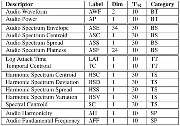
fea-ture (in the range of 10 ms–30 ms). For instance the spectral MPEG-7 descriptors Audio Spectrum Envelope (ASE), Au-dio Spectrum Centroid (ASC), and AuAu-dio Spectrum Spread (ASS) use a blocksize of 30 ms to obtain a higher frequency resolution. For spectral features, a Short-Time Fourier Trans-form (STFT) with a Hamming window is applied to each block. The 15 extracted MPEG-7 Audio Low-Level Descrip-tors [8] could be generally divided into: basic temporal, basic spectral, temporal timbre, spectral timbre, and signal param-eter descriptors listed in detail in Table 1. Especially, LAT is an important descriptor of typical onset times of musical instruments since it captures the logarithmic duration from signal start to the maximum or begin of the sustained signal

Descriptor Label Dim TB Category

Audio Waveform AWF 2 10 BT

Audio Power AP 1 10 BT

Audio Spectrum Envelope ASE 34 30 BS Audio Spectrum Centroid ASC 1 30 BS Audio Spectrum Spread ASS 1 30 BS Audio Spectrum Flatness ASF 24 10 BS

Log Attack Time LAT 1 10 TT

Temporal Centroid TC 1 10 TT Harmonic Spectrum Centroid HSC 1 30 TS Harmonic Spectrum Deviation HSD 1 30 TS Harmonic Spectrum Spread HSS 1 30 TS Harmonic Spectrum Variation HSV 1 30 TS Spectral Centroid SC 1 30 TS Audio Harmonicity AH 1 10 SP Audio Fundamental Frequency AFF 1 10 SP

Table 1: Overview of extracted MPEG-7 Audio Low-Level

Descriptors (Dim - dimensionality, TB- blocksize in ms, BT

- basic temporal, BS - basic spectral, TT - timbre temporal, TS - timbre spectral, SP - signal parameter)

Feature Label Dim TB Category

Specific Loudness Ld 24 20 PS

Sharpness Sh 1 20 PS

Spread Sp 1 20 PS

Mel Freq. Cepstral Coeff. MFCC 13 20 PS Zero Crossing Rate Z 1 20 PT Spectral Centroid Sc 1 20 S Spectral Width Sw 1 20 S Spectral Asymmetry Sa 1 20 S Spectral Flatness Sf 1 20 S Frequency Cutoff Fc 1 20 S Spectral Decrease Sd 1 20 S Spectral Oscillation So 1 20 S Spectral Slope Ss 1 20 S

Table 2: Overview of other extracted features (Dim -

dimen-sionality, TB blocksize in ms, PS perceptual spectral, PT

-perceptual temporal, S - spectral)

part. The other extracted audio features [9] could be gen-erally divided into: temporal, perceptual spectral, and other spectral features. They are shown in Table 2. All these fea-tures result in a 120-dimensional feature vector. They are extracted from both the original sounds and all the sounds altered by the considered modifications.

The motivation for the chosen signal modifications is given in Section 1. The parameters of all considered signal modifications are listed in Table 3. It should be noted that the signal modifications are applied to each audio signal without changing the sample frequency.

3. FEATURE SELECTION

Feature selection techniques [10, 11] aim at obtaining a sub-set of efficient features from a larger sub-set of candidate ones, where efficiency is determined by a chosen criterion. In general, the purpose of feature selection for classification problems is to maximize the classification accuracy. These techniques can be distinguished into filter and wrapper tech-niques. Filter techniques obtain their selection decisions

Label Parameter Value Unit Description

O - - - original L8 fc 8 kHz low-pass filtering L16 fc 16 kHz low-pass filtering M32 Bitrate 32 kb/s MP3 cod./dec. M64 Bitrate 64 kb/s MP3 cod./dec. M128 Bitrate 128 kb/s MP3 cod./dec. N30 SNR 30 dB AWGN N40 SNR 40 dB AWGN R1 RevTime 2000 ms reverberation Delay 1000 ms R2 RevTime 2000 ms reverberation Delay 800 ms R3 RevTime 1500 ms reverberation Delay 750 ms

Table 3: Overview of signal modifications with parameters from criteria computed with the initial features, whereas the feature selection decisions of wrapper techniques are directly based on the classification accuracy result. In this work, we consider two sequential filter techniques based on a Fisher-like criterion [11] and using two alternative subset search techniques known as sequential forward selection (SFS) and sequential backward selection (SBS). Since the rankings of SFS and SBS obtained from our experiments have only mi-nor differences at the last rank positions, we will only con-sider further the SFS algorithm and rankings. The objective measure for the SFS algorithm [11]

J=Tr(Sb)

Tr(Sw) (1)

is chosen in this work as a ratio between the trace of the

between-class scatter matrix Sband the trace of the

within-class scatter matrix Sw. Tr(Sb)is a measure of the average

distance (over all classes) of the mean of each class from the

global mean for all classes. Tr(Sw)is a measure for the

aver-age of variance of features. Therefore J measures the sepa-rability of classes for a given set of features. Great between-class spacing and small within-between-class variances lead to high class separability (high values of J).

The SFS algorithm generates a ranking of features or-dered by the highest class separability according to J in the following way: J is initially computed for each individual feature. The best feature (the one with the highest J) is first chosen. Subsequently, J is computed for all pairwise combi-nations with the first rank feature and all other remaining fea-tures. The combination with the highest separability is cho-sen and the first two ranks are determined. These two ranks build a new subset and the SFS algorithm proceeds with the computation of J for all combinations between this subset and one of all remaining features. Then again, the combi-nation with the maximum J is chosen and the next rank is determined. The SFS proceeds this way until the number of features that have to be selected is reached or the subset equals the set of available features. In the following, the al-gorithmic form of the SFS algorithm is presented. X is the set of all features.

Rk O L8 L16 M32 M64 M128 N30 N40 R1 R2 R3

1 LAT LAT LAT LAT LAT LAT LAT LAT LAT LAT LAT

2 MFCC-3 MFCC-3 MFCC-3 Ld-2 MFCC-3 MFCC-3 MFCC-3 MFCC-3 MFCC-3 MFCC-3 MFCC-3

3 Ld-2 Ld-2 Ld-2 MFCC-3 Ld-2 Ld-2 MFCC-4 MFCC-4 Ld-2 Ld-2 Ld-2

4 MFCC-4 MFCC-4 MFCC-4 MFCC-4 MFCC-4 MFCC-4 Ld-1 Ld-2 MFCC-4 MFCC-4 MFCC-4

5 Ld-1 Ld-1 Ld-1 Ld-1 Ld-1 Ld-1 Ld-2 Ld-1 ASC ASC ASC

6 ASC ASC ASC ASC ASC ASC MFCC-5 ASC Ld-1 Ld-1 Ld-1

7 MFCC-5 TC MFCC-5 TC TC MFCC-5 ASC TC MFCC-5 MFCC-5 MFCC-5 8 TC Sc TC HSC MFCC-5 TC TC MFCC-5 TC HSC TC 9 Sh Sh Sh Sh MFCC-6 Sh ASE-34 MFCC-6 Sh TC Sh 10 SC HSC SC SC HSC SC MFCC-6 SC Fc Sh Fc 11 MFCC-6 MFCC-5 MFCC-6 Sc SC MFCC-6 SC AWF-2 MFCC-6 Fc MFCC-6 12 Sa SC Sc Fc Sh Sa MFCC-1 MFCC-7 SC MFCC-6 SC 13 Fc MFCC-6 Sa MFCC-6 Sa Fc AWF-2 MFCC-1 HSC SC Sa

Table 4: Rankings of the 13 best features selected by SFS for original signals and all signal modifications. Features that differ from the ranking of the original signals (column O) are indicated bold.

Rk Feature 1 LAT 2 MFCC-3 3 Ld-2 4 MFCC-4 5 Ld-1 6 ASC 7 TC 8 MFCC-5 9 MFCC-6 10 SC 11 Sh 12 HSC 13 AWF-2

Table 5: The 13 best features of the robust feature ranking obtained by the average feature rank over all available modi-fied audio databases and the original one for each feature.

1. Start with the empty feature set Ys= {/0} with s = 0.

2. Out of the features that have not yet been chosen, select

the one feature f+_{that maximizes the objective function}

Jin combination with the previously selected features:

f+= _argmax

fi∈X −Ys

{J(Ys∪ fi)}.

3. Update: Ys+1=Ys∪ f+, s → s + 1.

4. Go to 2.

4. ROBUST FEATURE RANKING

How is it possible to identify robust features or obtain a ro-bust feature ranking for audio features automatically? To this end, we propose the following scheme. Various signal modi-fications should be introduced by applying various audio ef-fects to an initial “clean” database of audio classes. Fea-ture selection techniques are then applied to the original and each such modified audio database. Here, the feature selec-tion process can be stopped if the desired dimensionality is reached. The feature ranking for the original database along with the rankings for all modified databases are subsequently combined in a straightforward way. The robust feature ranks are ordered according to the average rank for each feature

where the average is computed over all available modified databases and the original one.

5. EXPERIMENTAL RESULTS

Approximately 6000 isolated notes of 14 different musical instruments with different pitch and playing styles are used as audio data. The instruments are woodwinds (bassoon, clar-inet, horn, flute, oboe), brass (tuba, trombone, trumpet, sax), strings (contrabass, cello, viola, violin), and piano. The au-dio data is part of the Musical Instrument Sound Database (RWC) [12].

After feature extraction, a feature ranking is created for each signal modification and the original audio data with SFS resulting in 11 rankings. The SFS is performed on

approx-imately 106_{frames for each signal modification. The Table}

4 lists the 13 best features for all signal modifications and the original audio data selected with SFS. Table 5 lists the 13 robust features that are selected by the average feature ranks over all effects as described in Section 4.

LAT has the highest class separability for all signal mod-ifications and the original signals. The work by Simmerma-cher et al. [5] shows the same result for original audio data with different feature selection methods on isolated notes. Their study shows further that the results for musical instru-ment classification on isolated notes can not easily be gener-alized to solos. Hence, the results may not apply to the even more complex case of polyphonic music. Nevertheless, note that the principle of our approach is not restricted to isolated notes, nor to the music instrument classification problem.

For isolated notes, also some of the lower MFCCs, the first two perceptual adapted loudness coefficients (Ld-1 and Ld-2), the spectral centroids (SC and ASC) and the temporal centroid (TC) have low ranks for all signal modifications and the original signals. The deviation of feature ranks over the SFS rankings corresponding to different signal modifications is relatively low for these mentioned features.

Furthermore, the maximum, minimum, mean, median, standard deviation, skewness, and kurtosis of each feature over all classes and for all signal modifications and the orig-inal database are extracted to explore their changes. Great

O L8 L16 M32 M64 M128 N30 N40 R1 R2 R3 0 0.1 0.2 0.3 0.4 0.5 0.6 0.7 0.8 0.9 1 Signal Modifcations Classification Accuracy Original/Robust MFCC (a) Dimensionality of 5 O L8 L16 M32 M64 M128 N30 N40 R1 R2 R3 0 0.1 0.2 0.3 0.4 0.5 0.6 0.7 0.8 0.9 1 Signal Modifcations Classification Accuracy Original Robust MFCC (b) Dimensionality of 13 O L8 L16 M32 M64 M128 N30 N40 R1 R2 R3 0 0.1 0.2 0.3 0.4 0.5 0.6 0.7 0.8 0.9 1 Signal Modifcations Classification Accuracy Original Robust (c) Dimensionality of 30

Figure 1: Classification accuracy for GMM classification experiments with original and robust features selected with SFS retaining the first 5, 13, and 30 features as well as MFCC for 5 and 13 features.

variations of the statistics of a feature over the different signal modifications suggest that this feature is highly influenced by this signal modifications and thus not very robust. The fea-tures LAT and TC show very small changes of their statistics, so the statistical evaluation supports the results of the robust feature ranking in Table 5. This features could be consid-ered as very robust features. Some of the lower MFCCs and the first two Ld coefficients (Ld-1 and Ld-2), SC, and ASC show some larger differences between the statistics for addi-tive noise, so they could be considered as some less robust features for noise, although they are among the 13 best fea-tures of the robust feature ranking, but they seem to be robust against all other signal modifications.

After evaluating the feature rankings, the classification accuracies of the robust feature scheme are compared to the ones relating to a classification scheme based on features

se-lected over the original database and to a third classification scheme using only MFCCs, as these are very common audio features. Since the robust features and the selected features of the original database do not differ for the dimensionality of 5, they are compared jointly to the first 5 MFCCs. For a dimensionality of 13, robust and original feature selections are compared to the first 13 MFCCs. For a dimensionality of 30, only the robust features are compared to the original feature selection.

Gaussian Mixture Models (GMMs) [11] are used as para-metric models for maximum likelihood (ML) classification. So a joint decision for all frames of each isolated note is taken to classify the musical instrument. The GMMs for each class of musical instrument have eight Gaussian com-ponents. They are trained with the well-known Expectation Maximization (EM) algorithm. For the training phase, we

choose to exploit only features extracted from the original audio data to put the focus on the contribution of a robust

feature selectionstage to the classification performance. All

classification experiments are performed with ten-fold cross-validation. Results in terms of average classification accura-cies are shown in Figure 1.

The results of the classification experiments show us that mainly lossy audio compression with low bit-rates (M32) and additive white Gaussian noise (N30 and N40) as signal mod-ifications affects the classification accuracy. For low dimen-sionality, we obtain the result that normal feature selection on original audio data lead to the same set of features as the robust feature ranking for the given audio classes and signal modifications. Therefore, the obtained classification accura-cies for the set of features selected from the original database are valid at the same time for the robust feature ranking. The set of the first five MFCCs could be outperformed for L8, M32, N40, and N30. Especially for N30, the gain in classi-fication accuracy with feature selection compared to the first five MFCCs is approximately 27 %. For a dimensionality of 13, the robust feature set can improve the classification ac-curacy up to 20 % for N30 compared to the original feature selection. Here, it is remarkable, that only two features of the original feature selection are replaced. Namely, Sa (Spec-tral Asymmetrie) and Fc (Frequency Cutoff) are replaced by HSC (Harmonic Spectrum Centroid) and AWF-2 (positive envelope).

For a higher dimensionality such as 30, it seems that fea-tures, which are highly affected by signal modifications such as noise, are again among the set of features that are sup-posed to be robust. However, the robustness is also a matter of the dimensionality and the available initial set of features. We observe that the greater number of 30 selected features (see Figure 1(c) compared with Figure 1(b)) leads to lower classification accuracies for N30 and N40. The classification accuracies for all other signal modifications and the original signals does not change significantly.

Furthermore the differences in accuracies between the features based on original audio data and the robust features are very small for all signal modifications. Using only a fixed set of features such as the first 13 MFCCs instead of using any feature selection technique at all can by chance lead to a robust classification system as Figure 1(b) shows for N30 and N40.

The proposed robust feature selection method is mostly useful when the feature dimensionality is very limited (as Figure 1(a) and Figure 1(b) show). Finally, the experimen-tal results show us in the main that our scheme to construct a robust set of features based on standard feature selection techniques is successful.

6. CONCLUSIONS AND FUTURE WORK An evaluation of robust audio features against common sig-nal modifications has been performed. For this purpose a method for the creation of a robust feature set has been pro-posed. The successful improvement of the classification

ac-curacy for modified signals has been proven in an experimen-tal evaluation. Further work will extend this method to more complex databases with solos or even polyphonic music as well as to other classification problems. Also we will con-sider training the classifiers on both the original and mod-ified audio data. Beyond features of frames, audio texture windows capturing long-term properties should be consid-ered further.

References

[1] J.J. Burred, M. Haller, S. Jin, A. Samour, and T. Sikora, “Audio content analysis,” in Semantic Multimedia and

Ontologies: Theory and Applications, Y. Kompatsiaris

and P. Hobson, Eds., chapter 5. Springer, 2008. [2] P. Herrera-Boyer, A. Klapuri, and M. Davy, “Automatic

classification of pitched musical instrument sounds,” in Signal Processing Methods for Music Transcription, pp. 163–200. Springer, 2006.

[3] S. Essid, G. Richard, and B. David, “Instrument recog-nition in polyphonic music based on automatic tax-onomies,” IEEE Transactions on Audio, Speech and

Language Processing, vol. 14, no. 1, pp. 68–80, 2006.

[4] G. Richard, P. Leveau, L. Daudet, S. Essid, and B. David, “Towards polyphonic musical instrument recognition,” in Proc. Int. Congress on Acoustics (ICA), 2007.

[5] C. Simmermacher, D. Deng, and S. Cranefield, “Fea-ture analysis and classification of classical musical in-struments: An empirical study,” in Advances of Data

Mining, 2006, Springer LNAI 4065, pp. 444–458.

[6] E. Benetos, M. Kotti, and C. Kotropoulos, “Musical in-strument classification using non-negative matrix fac-torization algorithms and subset feature selection,” in

Proc. ICASSP, 2006, vol. 5.

[7] S. Sigurdson, K.B. Petersen, and T. Lehn-Schiøler, “Mel frequency cepstral coefficients: An evaluation of robustness of mp3 encoded music,” in ISMIR 2006, Vi-coria, Canada, 2006.

[8] H.-G. Kim, N. Moreau, and T. Sikora, MPEG-7 audio and beyond: Audio content indexing and retrieval, John Wiley & Sons, 2005.

[9] G. Peeters, “A large set of audio features for

sound description (similiarity and classification) in the CUIDADO project,” in Proc. 115th AES Convention, 2004.

[10] I. Guyon and A. Elisseeff, “An introduction to variable and feature selection,” Journal of Machine Learning Research, vol. 3, pp. 1157–1182, 2003.

[11] S. Theodoridis and K. Koutroumbas, Pattern

Recogni-tion, Elsevier, 2006.

[12] M. Goto, H. Hashiguchi, T. Nishimura, and R. Oka, “RWC music database: Music genre database and mu-sical instrument sound database,” in Proc. ISMIR, 2003, pp. 229–230.