HAL Id: hal-00922522
https://hal-imt.archives-ouvertes.fr/hal-00922522
Submitted on 27 Dec 2013
HAL is a multi-disciplinary open access
archive for the deposit and dissemination of
sci-entific research documents, whether they are
pub-lished or not. The documents may come from
teaching and research institutions in France or
abroad, or from public or private research centers.
L’archive ouverte pluridisciplinaire HAL, est
destinée au dépôt et à la diffusion de documents
scientifiques de niveau recherche, publiés ou non,
émanant des établissements d’enseignement et de
recherche français ou étrangers, des laboratoires
publics ou privés.
Mixed-Criticality Multiprocessor Real-Time Systems:
Energy Consumption vs Deadline Misses
Vincent Legout, Mathieu Jan, Laurent Pautet
To cite this version:
Vincent Legout, Mathieu Jan, Laurent Pautet. Mixed-Criticality Multiprocessor Real-Time Systems:
Energy Consumption vs Deadline Misses. First Workshop on Real-Time Mixed Criticality Systems
(ReTiMiCS), Aug 2013, Taipei, Taiwan. pp.1-6. �hal-00922522�
Mixed-Criticality Multiprocessor Real-Time
Systems: Energy Consumption vs Deadline Misses
Vincent Legout, Mathieu Jan
CEA, LIST,
Embedded Real Time Systems Laboratory F-91191 Gif-sur-Yvette, France {vincent.legout,mathieu.jan}@cea.fr
Laurent Pautet
Institut Telecom TELECOM ParisTech LTCI - UMR 5141 Paris, France [email protected]
Abstract—Designing mixed criticality real-time systems raises numerous challenges. In particular, reducing their energy con-sumption while enforcing their schedulability is yet an open research topic. To address this issue, our approach exploits the ability of tasks with low-criticality levels to cope with deadline misses. On multiprocessor systems, our scheduling algorithm handles tasks with high-criticality levels such that no deadline is missed. For tasks with low-criticality levels, it finds an appropriate trade-off between the number of missed deadlines and their energy consumption. Indeed, tasks usually do not use all their worst case execution time and low-criticality tasks can reach their deadlines, even if not enough execution time was provisioned offline. Simulations show that using the best compromise, the energy consumption can be reduced up to 17% while the percentage of deadline misses is kept under 4%.
I. INTRODUCTION
Multiprocessor systems are now ubiquitous even on embed-ded systems and the number of cores per chip is still rising. With this constantly growing computing capacity, designers of embedded real-time systems aim to increase the number of functionalities. They also want to reduce the number of chips due to the economical constraints. This leads to the requirement of executing applications with different levels of criticality on a same multiprocessor chip. The real-time scheduling community recently looked at solutions to sched-ule such systems, commonly called Mixed-Criticality (MC) systems (e.g. [19], [6]).
Scheduling MC systems as traditional systems, where all tasks share the same criticality level, is possible but is over-pessimistic because it is equivalent to assume the highest level of criticality for all the tasks. The low-criticality tasks do not require this assumption: deadline misses are allowed to a certain degree as the failures are considered less severe. Such low-criticality tasks will be allowed to continue, while the system has to take remedial actions when a high-criticality task misses a deadline. Scheduling low-criticality tasks can therefore be made under more optimistic assumption. We use this ability of the low-criticality tasks to miss some of their deadlines to reduce the energy consumption of MC systems.
The energy consumption of embedded real-time systems is indeed an important concern to increase their autonomy because they are mainly powered by batteries. This work focuses on the energy consumption of processors which are
responsible, directly or indirectly, for the majority of the global energy consumption. Energy consumption is divided in dynamic consumption and static consumption. The former depends on the activity of the processor while the latter is mainly due to leakage current and can only be reduced by activating a low-power state. Several research works from Austin [3], Lesueur [14] or Awan [4] show that while dynamic consumption used to be preponderant, static consumption is now responsible for the majority of the energy consumption. According to Buttazzo and al. [13], the leakage current already accounted for 50% of the total power dissipation in 90 nm technologies and this trend is only increasing as the VLSI technology is scaling down to deep sub-micron domain. Thus, this work focuses on reducing static consumption.
In this work, we aim to reduce the consumption of MC embedded systems. We assume two levels of criticality and the objective is to be more aggressive while scheduling the low-criticality tasks. The rationale is that not guaranteeing offline the deadlines of all the low-criticality tasks is not a major issue, as the tasks (low and high-criticality) often do not use their Worst Case Execution Time (WCET) online. The generated slack time can therefore be used on-line by the other low-criticality tasks to meet their deadlines. The contribution of this paper is LPDPM-MC, a power-aware scheduling algorithm for MC multiprocessor systems which finds an appropriate trade-off between the number of deadline misses of the low-criticality tasks and their energy consumption. It is based on the LPDPM algorithm [15], a scheduling algorithm for multiprocessor systems. LPDPM has two properties: it is an optimal scheduling algorithm (i.e. it generates a correct schedule whenever the task set is feasible) and it reduces static consumption. This algorithm uses linear programming to compute the schedule offline.
A. Related Work
MC systems have first been introduced by Vestal [19] and Baruah and al. ([5], [6]). In addition to its deadline and period, a MC task also specifies its criticality level (χi) and a set of
WCETs. In this set, there is one WCET value per criticality level, up to χi, and higher the criticality level is, higher
is the WCET value. On uniprocessor systems and for static priority tasks, their objective is to improve the schedulability
of the low-criticality tasks while guaranteeing the deadlines of the high-criticality tasks. For multiprocessor systems, Li and Baruah [17] use global scheduling while the solution of Mollison and al. [18] use partitioned scheduling to assign tasks to processor using different strategies according to the level of criticality. Burns and Davis summarized the last researches on MC systems scheduling in [8].
However, to the best of our knowledge, no solution has been proposed to reduce the energy consumption of MC systems. For systems with only one level of criticality, several algorithms have been published using either a partitioned or a global approach. Huang and al. [12] first assign the tasks to processor but they may then be reallocated to another processor online to create large idle periods. For global scheduling, where the tasks can migrate, the only solution has been proposed by Bhatti and al. [7]. They try to use only one processor to activate the other processors only when required. However, all these solutions have a complexity which prevents them to be practicable (e.g. O(n3
) on each scheduling event for Bhatti, with n tasks). Besides, these scheduling algorithms are not optimal from the point of view of the CPU usage.
B. Outline
In the remainder of this paper, section II details the pro-cessor and the task model used. Section III describes how to compute a power-aware schedule, first step to reduce the energy consumption of MC systems. Then in section IV, we distinguish the low-criticality tasks from the high-criticality tasks and show how to set a tradeoff between energy and deadline miss for the low-criticality tasks. Finally, section V evaluates the solution and section VI concludes.
II. MODEL
A. Power model
We use a system with m identical processors and each processor has ns low-power states. In a low-power state, a processor cannot execute any instruction and its consumption is reduced. We further assume that each low-power state can be activated independently of the state of the other processors. This assumption prevents the use of a low-power state that deactivates a level of cache shared between a set of processors (typically the L2 cache or higher). We plan to remove this restriction in future work. However, such a deep low-power state is rarely available on embedded chips, since they have no or one level of cache. This statement is based on an analysis of the low-power states of the ARM Cortex processor family. The most efficient low-power state has index 0. The energy consumption of state s is Es. Coming back from a low-power
state to the active state requires a transition delay and the processor cannot execute any instruction while waking up. Let P ens be the consumption penalty to come back from
low-power state s. The more energy efficient a low-low-power state is, the more components are turned off and the more important is the consumption required to come back to the active state. Thus E0 < E1 < ... < Ens and P en0 > P en1 > ... >
P enns. To avoid having to deal with a particular case for the
idle mode, a fake power state was added when no low-power state can be activated. It has index ns and with Ens= 1
and P enns= 0. The minimum idle period for which activating
a given low-power state saves more energy than letting the processor idle is called the Break-Even time (BET). The BET of each low-power state s is BETs and BETns= 0.
B. Task Model
A set Γ of n independent, synchronous, preemptible and periodic tasks is scheduled on this system. Tasks can migrate from one processor to another. Each task τi has a Worst Case
Execution Time Ci(WCET), a period Tiand a criticality level
Li. Tasks have implicit deadlines, i.e. deadlines are equal to
periods. We consider two different criticality levels: high and low, like [6] and [17]. The task set hyper-period is named H and is the least common multiple of all periods of tasks in Γ. Utilization ui of task τi is the ratio CTi
i and the task set global utilization is the sum of all utilizations: U =Pn−1
i=0 ui.
UHI is the global utilization of high-criticality tasks, while ULO
is the global utilization of low-criticality tasks. A job j is an instance of a task and is also characterized by its WCET j.c, its deadline j.d and its criticality level j.l. The job set JΓ
contains all jobs of Γ scheduled during the hyper-period H. We assume m− 1 < U < m. Indeed, if U < m − 1, at least one processor can be put asleep to retrieve the assumption m− 1 < U < m. And if U = m, no low-power state can be activated.
C. Low-criticality tasks
As said earlier, the low-criticality tasks can miss some deadlines. The percentage of deadline misses depends on the criticality level of the task: the lower the criticality level is, the higher this percentage can be. To take advantage of this feature, we reserve only a percentage of the WCET of each low-criticality task. This percentage must be no less than α, with0 ≤ α ≤ 1. α × Ci is the minimal execution time which
must be reserved for each low-criticality task τi.
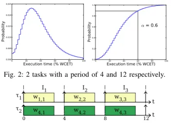
Choosing a value for α is not straightforward. A too small value increases the number of deadline misses up to a point where the low-criticality tasks might be useless to the system. A too large value would not be aggressive enough to generate an interesting reduction of energy consumption. The choice of α is the responsibility of the system designer as he wants to focus on the energy consumption or the schedulability of the low-criticality tasks. For example, α can be chosen such that the probability of the actual execution time to be larger than α× j.c is under a given percentage. Section V evaluates the efficiency of LPDPM-MC with 4 different values of α. Using a different α per low-criticality task could also be considered. In our evaluation, we rely on a Gumbel distribution (param-eters µ= 2 and β = 4) for the value of the actual execution time (AET) of the low-criticality tasks with regard to their WCET, as suggested in [9]. Figure 1 pictures the probability distribution (left) and the cumulative probability (right). For instance, the probability for the actual execution time to be larger that0.6 × W CET is 88%.
Fig. 1: Distribution of execution times for low-criticality tasks.
0 20 40 60 80 100 Execution time (% WCET) 0.000 0.005 0.010 0.015 0.020 0.025 Probability 0 20 40 60 80 100 Execution time (% WCET) 0.0 0.2 0.4 0.6 0.8 1.0 Probability α = 0.6
Fig. 2: 2 tasks with a period of 4 and 12 respectively.
τ1 t τ2 t 0 4 8 12 w1,1 w2,2 w3,3 w4,1 w4,2 w4,3 I1 I2 I3
In the end, our task model is different from the one introduced by Vestal in [19], as it has a different goal. Vestal improves the off-line schedulability guarantees of the low-criticality tasks, by introducing a low-low-criticality WCET for each high-criticality task. We decrease the deadline miss ratio of the low-criticality tasks, whose maximum allowed execution time are off-line constrained in order to reduce the energy consumption, by using the available slack time on-line.
D. Approach
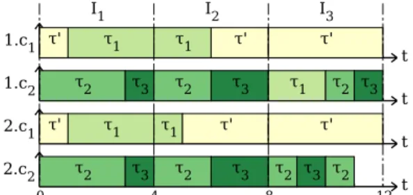
As in [16], the hyper-period is divided in intervals, an interval being delimited by two task releases. I is the set of intervals and|Ik| is the duration of the kthinterval. A job can
be present on several intervals, and we note wj,kthe weight of
job j on interval k. The weight of a job on an interval is the fraction of processor required to execute job j on interval k. Jk is the subset of JΓ that contains all active jobs in interval
k. Ej is the set of intervals on which job j can run. It must
contain at least one interval. The example task set in Figure 2 has two tasks and four jobs (jobs 1 to 3 from τ1and job 4 from
τ2). With this example, E4 is{I1, I2, I3} and J1 is{1, 4}.
Computing the complete schedule is a two steps process. First, the weights of all tasks on all intervals are computed with linear programming, using the WCET of tasks. The linear program consists of a set of linear constraints to ensure the system is schedulable and an objective function to reduce its energy consumption. Second, tasks are scheduled online inside intervals using the weights computed offline. The constraints required to guarantee the schedulability of the system are [16]:
∀k,X j∈Jk wj,k≤ m (1) ∀k, ∀j, 0 ≤ wj,k≤ 1 (2) ∀j,X k∈Ej wj,k× |Ik| = j.c (3)
The first inequality means that global utilization on an interval must not be larger the number of processors, thus any interval is schedulable. The second inequality forbids the
duration of a job on an interval to be negative or to exceed the length of the interval. This is necessary so that a task can be scheduled in an interval. Finally, the last equation guarantees that all jobs are completely executed.
Online, intervals are scheduled using FPZL (Fixed Priority until Zero Laxity) [10] where priorities are assigned to jobs according to their weight (the higher the weight the higher the priority). FPZL is a multiprocessor scheduling algorithm which is optimal with regard to processor utilization when all tasks share the same deadline. Section III then adds to the linear program an objective function to reduce the static consumption.
E. Idle time: taskτ′
To account for the time where processors are expected to be idle, an additional periodic task τ′
is added, as in [15]. τ′
has a period of H and a utilization of m− U , thus lower than 1. Let τ′
.c be its execution time on a hyper-period. Thus the task set now has n+ 1 tasks and U = m. The inequality in Equation (1) thus becomes an equality.
Inside intervals, the scheduling of τ′
is trivial when the weight of τ′
is either 0 or 1. However, when τ′
does not occupy a full interval, the execution of τ′
inside the interval plays a role in the reduction of the energy consumption. It should be executed either at the beginning or at the end of the interval. Indeed, when we merge this idle period with an idle period from a neighbor interval, we increase the opportunity to use deeper low-power states.
In our previous work [15], we used a heuristic to reduce the energy consumption (we minimized the number of pre-emptions of τ′
inside the hyper-period) and we scheduled online the execution of τ′
inside an interval. In this version of LPDPM, we refine this last step. We split τ′
into two subtasks which respective weights are computed in the linear program. The first subtask is executed at the beginning of the interval and the second at the end of the interval. This enables an offline computation of the best solution reducing the energy consumption based on the characteristics of each low-power state.
Let bk and ek be the weights of these two subtasks of τ′
in interval k with0 ≤ bk ≤ 1 and 0 ≤ ek ≤ 1. The weight
of τ′
in interval k is thus bk + ek, and an idle period lasts
for the whole interval k if bk+ ek= 1. To schedule intervals
online, these two subtasks are given the highest and lowest priorities, no matter their weight, so that they are executed at the beginning and at the end of the interval.
III. LPDPM:MINIMIZE STATIC CONSUMPTION
This section adds an objective function to the initial linear program to minimize the static consumption on a hyper-period. Doing the same computation on two hyper-periods would be more efficient because it would cover the transition between the two hyper-periods. However, the linear program would be twice as big for a very modest benefit.
To minimize the static consumption, the length of each idle period must be computed. An idle period in interval k starts
with the weight ek and can last over multiple intervals. When
ek = 0, the idle period may start in the next interval provided
bk+16= 0 because the two executions ek and bk+1 are always
connected. Let pk be the length of the idle period starting at
the interval k. pk is defined as follows:
pk=
(
ek× |Ik| + bk+1× |Ik+1| + pk+1 if bk+1+ ek+1= 1
ek× |Ik| + bk+1× |Ik+1| otherwise
(4) Thus the idle period of interval k is extended with the idle period starting at the end of interval k+ 1 (i.e. pk+1) when
bk+1+ ek+1 = 1 (i.e. τ′ occupies the full interval k + 1).
Then, we remove the idle periods which are counted twice and introduce an additional variable qk which gives the real
length of each idle period. Due to space constraint, we omit the details on how to compute qk.
To illustrate these notations, Figure 3 shows how to schedule task τ′
on an example which H = 16. The WCET of τ′
is 8. There are 4 intervals and ∀k, |Ik| = 4. The values of all
variables are shown in Table I. The column 0 represents the idle period starting with the execution of b1. Two idle periods
of length 6 and 2 are created in the end of intervals 1 and 3. The variable qk discards the idle period p2 as the first idle
period lasts across intervals 1 and 2.
TABLE I: Example with 4 intervals, τ′
.c= 8. k 0 1 2 3 4 bk∗ |Ik| 0 0 2 0 1 ek∗ |Ik| 0 2 2 1 0 pk 0 6 2 2 0 qk 0 6 0 2 0 Fig. 3: Schedule of τ′ from Table I. t 0 4 8 12 16 e 1 b2 e2 e3 b4 I 1 I2 I3 I4
To know which low-power state is used on each idle period, let LPs,k be a binary variable. LPs,k = 1 if the low-power
state s is activated during the idle period starting in the end of interval k and LPs,k= 0 otherwise. Each idle period must
activate a low-power state, thus: ∀k,X s LPs,k= ( 0 if qk = 0 1 otherwise (5)
A low-power state cannot be activated if the idle period is smaller than the BET. Thus this additional constraint:
∀k, ∀s, LPs,k= 0 if qk ≤ BETs (6)
The consumption while in low-power state s is Esand the
penalty consumption required to come back to the active state is P ens. Thus the consumption Pkof each idle period starting
at the end of interval k is: Pk=
X
s
LPs,k(Es× qk+ P ens) (7)
Minimizing the static consumption means minimizing on each interval the consumption of the idle task and also the
consumption of all tasks. Thus the final objective function of the mixed integer linear program is:
M inimizeX k (Pk+ X j∈Jk wj,k× |Ik|) (8)
IV. LPDPM-MC:HANDLE LOW-CRITICALITY TASKS
In this section, we take advantage of the ability of the low-criticality tasks to tolerate some deadline misses in order to further reduce the energy consumption.
A. Offline
Offline, the idea is to provision only a percentage of the WCET of each low-criticality task. The sum of all weights for each low-criticality job is no longer equal to the WCET of the job. Let tj be this difference:
tj= j.c −
X
Ej
wj,k (9)
A low-criticality job will suffer a deadline miss if its execution time is larger than the j.c− tj. If a low-criticality
job does not finish its execution before its deadline, the job is dropped. In the linear program, the low-criticality jobs are no longer constrained to Equation (3) but to equation:
∀j, α × j.c ≤ X
k∈Ej
wj,k× |Ik| ≤ j.c (10)
Note that α only represents the minimal percentage of the execution time which has to be reserved for each low-criticality task. It can therefore be higher than α× W CET . However, using α× W CET for all the low-criticality jobs gives the lowest consumption.
The execution times of the low-criticality jobs are reduced, thus the execution time of τ′
must also be increased to keep the global utilization equal to the number of processors. Thus, instead of Equation (3), τ′
is now constrained to: X
k
wτ′,k× |Ik| ≤ H (11)
Note that under these circumstances, the utilization of τ′
can be up to 1, i.e. its execution time equals to the hyper-period. However, requiring the utilization of τ′
to be no more than 1 bounds the reduction of the provisioned execution time that can be set using α for the low-criticality tasks. Thus, the reduction of the energy consumption is also bounded due to the following constraint:
UHI+ α × ULO≥ m − 1 (12)
To be more energy efficient, we get around this constraint by removing one processor from the system when m− 2 < UHI+ α × ULO< m− 1. The utilization of τ
′
therefore stays lower than 1 and all the computations are then done on m− 1 processors, including online scheduling. A processor is thus always in a lower-power mode with a consumption equals to zero but with an increasing risk of deadline misses. This process can be repeated to remove more processors if needed.
B. Online
Online, tasks may not use their WCET but their AET instead. It thus releases idle time, called slack time. This leads to the creation of lots of small idle periods which cannot be used to activate energy efficient low-power states. Instead, our online algorithm uses this slack time to schedule the low-criticality tasks. They get more execution time and are less likely to miss their deadlines. tj is used to know if a
low-criticality task can be executed based on the current amount of available slack time.
When a processor has no task to execute, our scheduling algorithm triggers the following actions in this order:
1) If the weight of τ′
in the current interval can be increased (i.e. its remaining execution time is less than the remaining time in the interval), the slack time is given to τ′
to increase the current idle period.
2) Else the slack time is used to execute available low-criticality jobs with tj >0. To keep the implementation
simple, the job with the smallest index is chosen. tj is
then updated while executing the job and the job ends its execution when tj = 0. Note that a job cannot be
selected if it is already executing on another processor. 3) Else a low-power state is activated (if compatible with BET constraints) according to the length of the forth-coming idle period.
This solution is aggressive because it gives a higher priority to the idle task instead of the low-criticality tasks to further re-duce the energy consumption. Note that the slack time created inside an interval is only used to extend the execution time of the low-criticality tasks of the given interval. An alternative strategy would anticipate the execution of the weights of current low-criticality tasks in the following intervals.
Figure 4 illustrates the possible scenarios with 3 tasks scheduled on 2 processors. We assume α = 0.5. Their criticality, WCET and period respectively are (high, 7, 12), (low, 8, 12) and (low, 2, 4). The AET of τ1and τ2respectively
are 4 and 7. And the AET of the three jobs of τ3respectively
are 1, 2 and 1. The execution times of the task set are shown in Table II. The first column of τj are the reserved execution
times, based on the weights of each job computed by the linear program for each interval. The total reserved execution time is 7 for τ2 and respectively 1, 2 and 1 for the 3 jobs of
τ3. As expected these values are not less than α× W CET .
The second column are the execution times consumed by the task when it uses its AET. If a job does not consume all its reserved execution time in an interval, its execution time on all subsequent intervals of the job is 0. τ′
b and τ ′
e are the two
subtasks of τ′
respectively executed at the beginning and at the end of the interval.
TABLE II: Execution times of the task set in Figure 4.
τ′
b τe′ τ1 τ2 τ3
I1 1 0 3 3 3 3 1 1
I2 0 2 2 1 2 2 2 2
I3 2 2 2 0 1 1 1 1
Fig. 4: Offline (1.cx) and online (2.cx) schedule on 2 cores.
1.c1 t 1.c2 t 2.c 1 t 2.c 2 t 0 4 8 12 τ' τ1 τ2 τ3 τ1 τ' τ2 τ3 τ' τ1 τ2 τ3 τ' τ1 τ2 τ3 τ1 τ' τ2 τ3 τ' τ2 τ3 τ2 I1 I2 I3
In the first two lines of Figure 4, tasks use their WCET. Thus τ2 misses its deadline, while τ3 misses its deadline in its first
and third jobs. In the last 2 lines, tasks use their AET. Thus in t= 5, when τ1 ends its execution, the slack time is given to
τ′
. τ1 finishes its execution in I2 and is thus not executed in
I3. τ2 and τ3 use their reserved execution time until t= 10,
therefore τ3 finishes. Then the slack time is given to τ2 to
finish its execution because τ′
is already executed on the first processor. And at t= 11, there is no other solution than trying to activate a low-power state if the idle period is large enough. No deadlines is thus missed for this scenario.
V. EVALUATION
We use a simulator to generate random task sets, with a global utilization set between 3 and 4. Each task set is scheduled on 4 processors and includes 3 high-criticality tasks and 7 low-criticality tasks. For each task set, the utilization of both high and low-criticality tasks is computed randomly between 0.01 and 0.99 with a uniform distribution using the UUniFast-Discard algorithm from Davis and Burns [11]. The period of each task is also chosen randomly between 10ms and 100ms with a uniform distribution. The task sets with a hyper-period larger than 10s are rejected to remain in a realistic bound of typical industrial systems. We allowed 5 minutes to IBM ILOG CPLEX to solve the linear program, which was enough to get a solution.
For each utilization value, 500 random task sets are gener-ated and scheduled by two global multiprocessor schedulers: LPDPM-MC and LPDPM [15]. We are not aware of any power-aware MC scheduling algorithm which could be used as a reference. For the simulation, we assume that the high-criticality tasks use their WCET. Four different values of α are used for LPDPM-MC: 0.2, 0.4, 0.6 and 0.8. Setting α to 0.2 and 0.4 is more aggressive because the probabilities for the actual execution time to be less than 0.2 × W CET and 0.4 × W CET are respectively only 20% and 60%. The other values are more conservative because this percentage grows respectively up to85% and 96%.
Table III describes the characteristics of the low-power states we consider in our simulations. The definition of these three states as well as their energy consumption and their transition delay is based on an analysis of the hardware capabilities of the STM32L [2] and the MPC551x [1].
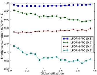
Figure 5 plots the mean global energy consumption of LPDPM-MC for each value of α. All consumptions are relative to the consumption of LPDPM, which is therefore always 1. It
TABLE III: Low-power states used for the simulation.
State Energy consumption Transition delay (ms)
Run 1
Sleep 0.5 0.1
Stop 0.1 2
Standby 0.00001 10
Fig. 5: Global energy consumption with 4 values of α.
3.0 3.2 3.4 3.6 3.8 4.0 Global utilization 0.60 0.65 0.70 0.75 0.80 0.85 0.90 0.95 1.00 Energy consumption (LPDPM = 1) LPDPM-MC (0.8) LPDPM-MC (0.6) LPDPM-MC (0.4) LPDPM-MC (0.2)
includes the consumption while processors are idle and while executing the low-criticality tasks. But it does not include the consumption while executing the high-criticality tasks which is identical for all the schedulers. LPDPM-MC with α= 0.2 is the most efficient scheduler with an energy consumption reduction up to35%. When α grows, the energy efficiency of the scheduler is reduced but is still 17% for α = 0.4 and up to10% for α = 0.6. The energy consumption improvement is almost null for α= 0.8.
We also computed the deadline miss ratio, i.e. the ratio between the number of deadline misses and the total number of jobs for low-criticality tasks only. The highest ratio of deadline misses, from 10% up to 28%, is obtained when α = 0.2. As expected, when α increases, the deadline miss ratio decreases. The ratio is between 2% and 5% when α = 0.4 and goes below 2% when α > 0.4. Based on these results, choosing α= 0.4 seems appropriate to significantly reduce the energy consumption while keeping a low ratio of deadline misses.
VI. CONCLUSION
This paper introduces LPDPM-MC, a multiprocessor real-time scheduling algorithm to reduce the energy consumption of mixed-critical systems. Offline, it only reserves a percentage of the WCET of the low-criticality tasks. The slack time generated online by tasks is then used to reduce the ratio of deadline miss for these low-criticality tasks. The designer can control the aggressiveness of the solution depending on whether the focus should be on reducing the energy con-sumption or the deadline misses. Results show that LPDPM-MC can be 17% more energy efficient than the non mixed-critical aware scheduling algorithms using the same approach, while the deadline miss ratio is lower than4%. Higher energy efficiency is achievable but with higher deadline miss ratios.
In a future work, we would like to evaluate the tradeoff given by LPDPM-MC when using others distributions for the AET of tasks. To be more flexible, it would be interesting to allow different values of α, one for each task. Another idea would be to fix as an objective the energy consumption reduction compared to LPDPM. The output will then be the largest possible value of α for the low-criticality tasks fulfilling this objective. Finally, we plan to integrate conditions to better take advantage of the low-power states that must be activated on all processors simultaneously.
REFERENCES
[1] FreeScale MPC5510 Microcontroller Family Reference Manual. [2] ST Microelectronics STM32L151xx and STM32L152xx advanced
ARM-based 32-bit MCUs Reference Manual.
[3] T. Austin, D. Blaauw, S. Mahlke, T. Mudge, C. Chakrabarti, and W. Wolf. Mobile supercomputers. Computer, 37(5):81–83, May 2004. [4] M. Awan and S. Petters. Energy aware partitioning of tasks onto a
heterogeneous multi-core platform. In Proc. of the 19th IEEE
Real-Time and Embedded Technology and Applications Symp., 2013. [5] S. K. Baruah, V. Bonifaci, G. D’Angelo, H. Li, A.
Marchetti-Spaccamela, N. Megow, and L. Stougie. Scheduling real-time mixed-criticality jobs. In Proc. of the 35th Int. Conf. on Mathematical
foundations of computer science, pages 90–101, 2010.
[6] S. K. Baruah, A. Burns, and R. I. Davis. Response-time analysis for mixed criticality systems. In Proc. of the IEEE 32nd Real-Time Systems
Symp., pages 34–43, 2011.
[7] M. Bhatti, M. Farooq, C. Belleudy, and M. Auguin. Controlling energy profile of rt multiprocessor systems by anticipating workload at runtime. In Proc. of SYMPosium en Architectures nouvelles de machines, 2009. [8] A. Burns and R. Davis. Mixed criticality systems - a review, 2013. [9] L. Cucu-Grosjean, L. Santinelli, M. Houston, C. Lo, T. Vardanega,
L. Kosmidis, J. Abella, E. Mezzetti, E. Quinones, and F. Cazorla. Measurement-based probabilistic timing analysis for multi-path pro-grams. In Proc. of the 24th Euromicro Conf. on Real-Time Systems, pages 91–101, 2012.
[10] R. Davis and A. Burns. Fpzl schedulability analysis. In Proc. of the 17th
IEEE Real-Time and Embedded Technology and Applications Symp., pages 245 –256, 2011.
[11] R. I. Davis and A. Burns. Improved priority assignment for global fixed priority pre-emptive scheduling in multiprocessor real-time systems.
Real-Time Systems, 47(1):1–40, Jan. 2011.
[12] H. Huang, F. Xia, J. Wang, S. Lei, and G. Wu. Leakage-aware reallocation for periodic real-time tasks on multicore processors. In Proc.
of the 5th Int. Conf. on Frontier of Computer Science and Technology, pages 85–91, 2010.
[13] K. Huang, L. Santinelli, J.-J. Chen, L. Thiele, and G. C. Buttazzo. Ap-plying real-time interface and calculus for dynamic power management in hard real-time systems. Real-Time Systems, 47, March 2011. [14] E. Le Sueur and G. Heiser. Dynamic voltage and frequency scaling:
The laws of diminishing returns. In Proc. of the Work. on Power Aware
Computing and Systems, pages 1–8, 2010.
[15] V. Legout, M. Jan, and L. Pautet. An off-line multiprocessor real-time scheduling algorithm to reduce static energy consumption. In Proc. of
the 1st Work. on Highly-Reliable Power-Efficient Embedded Designs, 2013.
[16] M. Lemerre, V. David, C. Aussagu`es, and G. Vidal-Naquet. Equivalence between schedule representations: Theory and applications. In Proc. of
the IEEE Real-Time and Embedded Technology and Applications Symp., pages 237–247, 2008.
[17] H. Li and S. Baruah. Global mixed-criticality scheduling on multipro-cessors. In Proc. of the 24th Euromicro Conf. on Real-Time Systems, pages 166–175, 2012.
[18] M. S. Mollison, J. P. Erickson, J. H. Anderson, S. K. Baruah, and J. A. Scoredos. Mixed-criticality real-time scheduling for multicore systems. In Proc. of the 10th IEEE Int. Conf. on Computer and Information
Technology, pages 1864–1871, 2010.
[19] S. Vestal. Preemptive scheduling of multi-criticality systems with varying degrees of execution time assurance. In Proc. of the 28th IEEE