HAL Id: hal-00876030
https://hal.inria.fr/hal-00876030
Submitted on 23 Oct 2013
HAL is a multi-disciplinary open access
archive for the deposit and dissemination of
sci-entific research documents, whether they are
pub-lished or not. The documents may come from
teaching and research institutions in France or
abroad, or from public or private research centers.
L’archive ouverte pluridisciplinaire HAL, est
destinée au dépôt et à la diffusion de documents
scientifiques de niveau recherche, publiés ou non,
émanant des établissements d’enseignement et de
recherche français ou étrangers, des laboratoires
publics ou privés.
Learning A Tree-Structured Dictionary For Efficient
Image Representation With Adaptive Sparse Coding
Jérémy Aghaei Mazaheri, Christine Guillemot, Claude Labit
To cite this version:
Jérémy Aghaei Mazaheri, Christine Guillemot, Claude Labit. Learning A Tree-Structured Dictionary
For Efficient Image Representation With Adaptive Sparse Coding. ICASSP - 38th International
Con-ference on Acoustics, Speech, and Signal Processing, May 2013, Vancouver, Canada. �hal-00876030�
LEARNING A TREE-STRUCTURED DICTIONARY FOR EFFICIENT IMAGE
REPRESENTATION WITH ADAPTIVE SPARSE CODING
J´er´emy Aghaei Mazaheri, Christine Guillemot, and Claude Labit
INRIA Rennes, Campus universitaire de Beaulieu 35042 Rennes Cedex, France
ABSTRACT
We introduce a new method, called Tree K-SVD, to learn a tree-structured dictionary for sparse representations, as well as a new adaptive sparse coding method, in a context of im-age compression. Each dictionary at a level in the tree is learned from residuals from the previous level with the K-SVD method. The tree-structured dictionary allows efficient search of the atoms along the tree as well as efficient coding of their indices. Besides, it is scalable in the sense that it can be used, once learned, for several sparsity constraints. We show experimentally on face images that, for a high sparsity, Tree K-SVD offers better rate-distortion performances than state-of-the-art ”flat” dictionaries learned by SVD or Sparse K-SVD, or than the predetermined overcomplete DCT dictio-nary. We also show that our adaptive sparse coding method, used on a tree-structured dictionary to adapt the sparsity per level, improves the quality of reconstruction.
Index Terms— Dictionary learning, tree-structured dic-tionary, sparse coding, sparse representations, image coding.
1. INTRODUCTION
Sparse representation of a signal consists in representing a signal y ∈ <n as a linear combination of columns, known as
atoms, from a dictionary matrix. The dictionary D ∈ <n×K
is generally overcomplete and contains K atoms. The ap-proximation of the signal can thus be written y ≈ Dx and is sparse because a small number of atoms of D are used in the representation, meaning that the vector x has only a few non-zero coefficients.
The choice of the dictionary is important for the repre-sentation. A predetermined transform matrix can be chosen. Another option is to learn the dictionary from training signals to get a well adapted dictionary to the given set of training data. As shown in [1], learned dictionaries have the potential to outperform the predetermined ones.
Sparse representations and dictionary learning are com-monly used for denoising [2, 3]. The application considered in this paper is image compression. This case has already been treated in [1, 4, 5], however with different dictionary construction methods, and different coding algorithms. In that context, for each signal y, a sparse vector x has to be
This work was supported by EADS Astrium.
coded and transmitted, which is equivalent to send a few pairs of atom index and coefficient value.
Recently, tree-structured dictionaries appeared [6, 7, 5]. In [6], the tree is considered as a unique dictionary, each node corresponding to an atom, and the atoms used for a signal representation are selected among a branch of the tree. The learning algorithm proceeds in two steps which are iterated: sparse coding using proximal methods and update of the en-tire dictionary. Even if it gives good results for denoising, the fact to consider the tree as a single dictionary makes it, in its current state, not well adapted to efficiently code the indices of the atoms when the dictionary becomes large. An-other kind of tree-structured dictionary, more adapted to the coding issue because structured as a tree of dictionaries, is TSITD (Tree-Structured Iteration-Tuned Dictionary) [5]. It constructs a tree-structured dictionary adapted to the itera-tive nature of greedy algorithms, such as the matching pursuit [8, 9, 10]. The concept of using a different dictionary for each iteration of the pursuit algorithm has been first expressed with Basic ITD (BITD) [7] structured in only one branch, each dic-tionary being learned from the residuals of the previous level with the K-means algorithm.
This paper first describes a new tree-structured dictionary learning method called Tree K-SVD. Inspired from ITD and TSITD, each dictionary at a given level is learned from a sub-set of residuals of the previous level using the K-SVD algo-rithm. The tree structure enables the learning of more atoms than in a ”flat” dictionary, while keeping the coding cost of the index-coefficient pairs similar. Tests are conducted on fa-cial images, as in [1, 4, 5], compressed for multiple rates in a compress scheme. Thus, for a given bit rate, Tree K-SVD is shown to outperform ”flat” dictionaries (SVD, Sparse K-SVD and the predetermined (over)complete DCT dictionary) in terms of quality of reconstruction for a high sparsity, i.e. when the number of atoms used in the representation of a vector is low. Setting the sparsity constraint to only a few atoms limits the number of levels, and so of atoms, in the tree-structured dictionary. The paper then describes an adap-tive sparse coding method applied on the tree-structured dic-tionary to adapt the sparsity per level, i.e. to allow selecting more than 1 atom per level. It is shown to improve the quality of reconstruction.
structure, the learning algorithm and its usage for sparse rep-resentations. In Section 3, we present our new adaptive sparse coding method. In Section 4, we then compare Tree K-SVD to state-of-the-art methods learning ”flat” or tree-structured dictionaries and to a predetermined dictionary. We also show the performances of the adaptive sparse coding. Finally, in Section 5, we conclude and discuss several future works.
2. A TREE-STRUCTURED DICTIONARY LEARNING METHOD
2.1. The tree structure
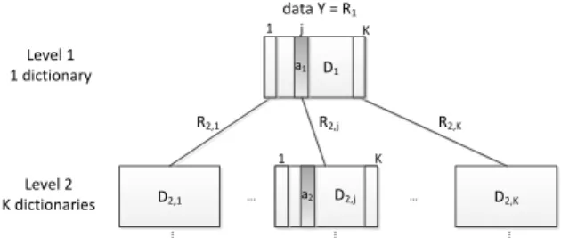
Tree K-SVD is a method learning a tree-structured dictionary from a training set of signals. It is then used to approximate a signal as a linear combination of atoms in the dictionary. The tree-structured dictionary is composed of L levels of 1, K, K2, ..., KL−1dictionaries of K atoms (Fig.1).
An advantage of the Tree K-SVD method is its scalability in sparsity. A ”flat” dictionary learned with K-SVD or Sparse K-SVD is learned for a specific sparsity constraint, that is a number of atoms to use in the approximation of a signal. Then, the dictionary is usually used to approximate signals with this sparsity constraint, in order to make the approxima-tion more efficient. In contrast, a tree-structured dicapproxima-tionary is learned with the Tree K-SVD method for a given number of levels, and such a dictionary with L levels can be used to approximate signals with a number of atoms from 1 to L.
data Y = R1 D2,K D1 D2,j D2,1 R2,1 R2,j R2,K Level 1 1 dictionary Level 2 K dictionaries ... ... .. . 1 a1 K 1 K .. . .. . a2 j
Fig. 1: The Tree K-SVD dictionary structure. 2.2. The dictionary learning algorithm
A tree-structured dictionary is learned with a top-down ap-proach: each dictionary in the tree is learned on residuals of the previous level with K-SVD [1], a state-of-the-art dictio-nary learning method. The sparsity constraint of K-SVD is set to 1 as only 1 atom can be selected per dictionary in our method. Of course, other dictionary learning methods than K-SVD could be used to learn each dictionary in the tree.
At the first level, the only dictionary D1is learned with
K-SVD from the training data Y , and with a sparsity constraint of 1 atom. Then OMP [9] is applied with a sparsity constraint of 1 to approximate each training signal in Y with only 1 atom from D1. Note that we use OMP for its simplicity and
fast execution but another pursuit algorithm could be used. Residuals (R2) are computed and then split in K residuals
(R2,1, ..., R2,K) to form one set of residuals per column of
D1. Each vector of R2 is put in R2,k, k ∈ [1, ..., K], if it
is a residual of the approximation of a vector in Y with the
column k in D1. Thus, the residuals of the column k, R2,k,
correspond to the residuals of the data vectors which are the most correlated to this column k in the dictionary D1. At
the second level, a dictionary is learned from each residuals set R2,kwith K-SVD. That way, the second level counts K
dictionaries. Each residuals set R2,k is then approximated
with 1 atom from the corresponding dictionary D2,k, with a
non-zero coefficient, to get K sets of residuals per dictionary at the second level. So there are K2 sets of residuals at the
third level, used to learn the K2dictionaries of the third level.
And so on. With this method, the dictionaries at a level are adapted to the residuals of the previous level.
Some dictionaries in the tree can be empty if the corre-sponding atom at the previous level is not used in any approx-imation of the previous residuals. Some can have a number of atoms inferior to K if the number of residual vectors used for the learning of these dictionaries is inferior to K. In that case, the residual vectors are simply copied, with normaliza-tion, and the learning of the branch is stopped.
2.3. Usage for sparse representations
Once a tree-structured dictionary of L levels has been learned from learning data, this dictionary can be used to approximate a vector by a linear combination of l atoms in the dictionary, with l ≤ L. The sparsity constraint l indicates how deep to go through the tree to select the best atoms. Indeed, 1 atom is se-lected at each level of the tree, starting with the first level. To select the atoms and compute the corresponding coefficients, we use the OMP algorithm as for the learning.
To represent a vector y as a linear combination of 2 atoms for example, with the tree-structured dictionary on Fig.1, first OMP is applied to y and the dictionary D1 with a sparsity
constraint of 1 atom. OMP gives the most correlated atom to y in D1, in the example a1, and the associated coefficient α1.
Residuals r = y − a1α1are computed. As the atom chosen
at the first level is a1, at the column j in D1, we necessarily
search for the second atom at the second level in the jth dic-tionary D2,j. Then, OMP is applied on the residuals r and
the dictionary D2,j to find the most correlated atom to r in
D2,j, a2, and the associated coefficient α2. The residuals are
updated to r = r − a2α2. Finally, the vector y can be written
y = a1α1+ a2α2+ r, with r the residuals.
The tree structure offers a good property to code the in-dices of the atoms aiused in the approximation of a vector.
Indeed, only the indices in small dictionaries in the tree have to be coded and not which dictionary to use at each level as the choice of an atom at a level forces the choice of the dic-tionary at the next level.
The tree structure offers also efficient sparse coding even if the dictionary is large. Indeed, OMP is applied on the small dictionaries in the tree and not on the entire tree. For each vec-tor to approximate, a single branch in the tree is used. Thus, it is similar in terms of complexity to realize sparse coding on a tree of dictionaries of K atoms than on a single ”flat” dictionary of K atoms.
3. ADAPTIVE SPARSE CODING PER LEVEL We introduce in this paper a new sparse coding method to search for atoms in tree-structured dictionaries. The sparse coding used in the ITD methods [7, 5] and that we presented in the previous section selects 1 atom per level of the tree. Thus, the maximum number of atoms that can be used in the representation is the number of levels in the tree. But to go too deep in the tree to select more atoms makes the number of dictionaries in the tree explode. The adaptive sparse coding allows selecting more than 1 atom per level and thus using more atoms in the representation with the same dictionary.
At each level, once a first atom has been selected, a choice is made between staying at the same level in the same dic-tionary to select another atom or going to the next level in the tree. For that, the 2 most correlated atoms to the current residual vector are found, one at the same level and the other one at the next level. The atom minimizing the energy of the residuals is kept in the representation. That way, the sparsity per level is automatically adapted to decrease the distortion.
4. RESULTS 4.1. Experimental setup
We use the Yale Face Database [11], containing 165 grayscale images in GIF format of 15 individuals. There are 11 im-ages per subject, one per different facial expression or con-figuration. 14 individuals, so 154 images, are used as train-ing data to learn the dictionary. The remaintrain-ing 11 images from the 15th individual are used as a test set. The train-ing images, with a size of 320x243 pixels, have been slightly cropped to the size of 320x240 pixels to cut the images in non-overlapping 8x8 pixels blocks. Each block is put as a vector to get the 184800 training vectors. The test images have been cropped to a size of 160x208 pixels to focus on the face. Thus, there are 5720 test vectors.
The reference dictionaries are learned in 50 iterations, as the dictionaries in TSITD and BITD. For Tree K-SVD, the first level is learned in 50 iterations and 10 iterations are enough for the next levels. K-SVD is initialized with the DCT dictionary, as the base dictionary of Sparse K-SVD, whose sparse dictionary is initialized by the identity matrix. Each dictionary in Tree K-SVD is initialized with the DCT dictionary also. For TSITD and BITD, the DCT dictionary or learning vectors are used for the initialization, according to the number of learning vectors.
Note that in the tests, for ”flat” dictionaries, the sparsity constraint (maximum number of atoms) used to approximate a test vector is the same as the one used to learn the dictionary. 4.2. Comparison with ”flat” dictionaries
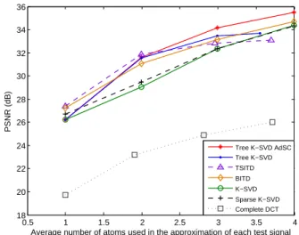
In order to compare the methods, we look at the influence of sparsity on the quality of representation. We first learn a dic-tionary on the training data for each sparsity constraint value between 1 and 4 atoms (to limit the number of levels in the tree), and then use the dictionaries to approximate the test
0.5 1 1.5 2 2.5 3 3.5 4 18 20 22 24 26 28 30 32 34 36
Average number of atoms used in the approximation of each test signal
PSNR (dB) Tree K−SVD AdSC Tree K−SVD TSITD BITD K−SVD Sparse K−SVD Complete DCT
Fig. 2: Sparse representations with Tree K-SVD and refer-ence dictionaries (K=64) (AdSC = with Adaptive Sparse Cod-ing).
data with the same sparsity constraint value. To approximate the test data, OMP is used to select the atoms and compute the non-zero coefficients. For Tree K-SVD, only one tree-strcutured dictionary of four levels is learned. Tree K-SVD is compared to the K-SVD dictionary [1], the Sparse K-SVD dictionary[3] with an atom sparsity set to 32, and also to a pre-determined dictionary, the (over)complete DCT basis. The K-SVD dictionary and the Sparse K-K-SVD dictionary are learned using the software made available by the authors [12, 13].
In the context of compression, we do not intend to com-pare the methods with the same total number of atoms, but with an equivalent coding cost of the indices. So for the ”flat” dictionaries, K is the total number of atoms, whereas for Tree K-SVD, TSITD and BITD, it is the number of atoms per dic-tionary in the tree.
Tree K-SVD outperforms the state-of-the-art ”flat” dictio-nary learning methods (Fig.2) when the sparsity constraint is at least 2 atoms and remains limited. Indeed, with a sparsity constraint of 1 atom, only the first level in the tree is used and Tree K-SVD is equivalent to a ”flat” dictionary learned with K-SVD with a sparsity constraint set to 1 atom. For dic-tionaries of 64 atoms (K=64) (Fig.2), Tree K-SVD offers a better quality of reconstruction for a sparsity constraint of 2 or 3 atoms. But the fourth atom in the approximation does not increase the quality of reconstruction as much as the pre-vious atoms. Deep in the tree, the residuals become too weak and the dictionaries too adapted to the training data. Besides, many dictionaries are incomplete and so less efficient. Regu-larly in the approximation, only 3 atoms are selected instead of 4 if an empty dictionary is found at the fourth level, hence an average of about 3.5 atoms instead of 4 atoms used in the approximation (Fig.2). The same behaviour can be seen with dictionaries of 256 atoms. Moreover, the learned dictionaries, adapted to the training data, give much better results than the predetermined DCT one.
4.3. Comparison between tree-structured dictionaries When we compare Tree K-SVD with TSITD (Fig.2), we ob-serve close results. The gap for a sparsity constraint of 1 atom is mainly due to the use of a function in K-SVD to replace the less useful atoms at the end of each iteration of the algorithm, that is inefficient for this sparsity constraint. Then when 3 or 4 atoms are used in the representation, Tree K-SVD takes the advantage on TSITD. It can be explained by a strategy used in TSITD to learn dictionaries in the tree. Indeed, in the case where the number of training vectors is too low to learn a dictionary of K atoms, we decide in Tree K-SVD to copy these training vectors in the dictionary. Whereas TSITD learns in that case a smaller dictionary than Tree K-SVD. These smaller dictionaries in the tree, when that case hap-pens, explain the lower quality of reconstruction of TSITD when 3 or 4 atoms are used in the approximation. Tree K-SVD gives also better results than BITD for 2 or 3 atoms. But BITD, structured in one branch of dictionaries, is then better for more than 3 atoms (Fig.2).
Tree K-SVD with the adaptive sparse coding (AdSC) clearly outperforms the original Tree K-SVD, TSITD and BITD for a high sparsity and when more than 2 atoms are used in the representation (Fig.2). Thus, the possibility to select more than 1 atom per level increases the performances. It also enables using more atoms in the representation, with the same dictionary, to reach a better quality if necessary. 4.4. Sparse representations for compression
In order to use sparse representations for compression, l (spar-sity constraint) coefficients and indices of atoms are coded for each test vector. The coefficients are first quantized with a uniform scalar quantizer with a dead zone. The quantized coefficients are put in a sequence, an End OF Block code sep-arating the coefficients of each test vector. The sequence is then encoded using a Huffman entropy coder, similarly to the JPEG coder and with the same Huffman code table. Finally, the rate of the indices is added. For each index, the rate is R = log2(K), with K the number of atoms per dictionary.
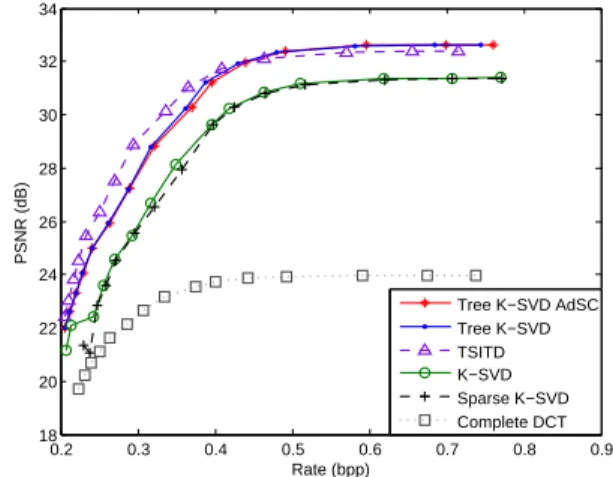
By sweeping through various values of the quantization step, we obtain the values of the R-D curves for the Tree K-SVD method and the state-of-the-art ones. The Tree K-K-SVD dictionary outperforms the ”flat” dictionaries when a small number of atoms is used in the representation, for complete (Fig.3), and overcomplete (Fig.4) dictionaries. The rate of Tree K-SVD with adaptive sparse coding (AdSC) is penal-ized by a flag in the bitstream of 1 bit per atom selected in the representation indicating if the next atom is selected at the same level or at the next one. However, this adaptive sparse coding method allows reaching a better quality (Fig.3) but is effective when more than 2 atoms are selected in the repre-sentation. That is why Tree K-SVD and Tree K-SVD AdSC reach about the same PSNR on Fig.4. The rate of TSITD is a bit lower but this method does not reach the same quality of reconstruction than Tree K-SVD and Tree K-SVD AdSC, especially for small dictionaries (Fig.3 and 4).
0.1 0.2 0.3 0.4 0.5 0.6 0.7 0.8 0.9 1 18 20 22 24 26 28 30 32 34 36 Rate (bpp) PSNR (dB) Tree K−SVD AdSC Tree K−SVD TSITD K−SVD Sparse K−SVD Complete DCT
Fig. 3: Rate-distortion curves for Tree K-SVD and reference dictionaries (K=64). The sparsity constraint is set to 3, mean-ing that each test signal is approximated by a maximum of 3 atoms from the dictionary.
0.2 0.3 0.4 0.5 0.6 0.7 0.8 0.9 18 20 22 24 26 28 30 32 34 Rate (bpp) PSNR (dB) Tree K−SVD AdSC Tree K−SVD TSITD K−SVD Sparse K−SVD Complete DCT
Fig. 4: Rate-distortion curves for Tree K-SVD and reference dictionaries (K=256). The sparsity constraint is set to 2.
5. CONCLUSION
In this paper, we presented a new method to learn a tree-structured dictionary. We have shown that Tree K-SVD out-performs ”flat” dictionaries learned by the methods K-SVD or Sparse K-SVD and the predetermined (over)complete DCT dictionary, when a small number of atoms is used in the rep-resentation. Thanks to the tree-structure, the search for the atoms and the coding of their indices is efficient. Finally, it is scalable in the sense that it can be used, after the learning, for several sparsity constraints. We have also shown that us-ing the adaptive sparse codus-ing, to select more than 1 atom per level, increases the performances.
The tree-structured dictionary learned comprises a large total number of atoms. But it could be possible to prune the tree by stopping the learning in a branch if it is considered that going deeper in the tree does not improve the quality enough. For each test vector, we could also imagine to select a variable number of atoms, that is to go more or less deep in the tree, according to the required quality and the available rate. Tests have been here realized on face images but will be applied in the future to other types of images, like satellite images.
6. REFERENCES
[1] M. Aharon, M. Elad, and A. Bruckstein, “K-SVD: an algorithm for designing overcomplete dictionaries for sparse representation,” IEEE Transactions on Signal Processing, vol. 54, no. 11, pp. 43114322, 2006. [2] M. Elad and M. Aharon, “Image denoising via sparse
and redundant representations over learned dictionar-ies,” IEEE Transactions on Image Processing, vol. 15, no. 12, pp. 37363745, 2006.
[3] R. Rubinstein, M. Zibulevsky, and M. Elad, “Double sparsity: Learning sparse dictionaries for sparse signal approximation,” IEEE Transactions on Signal Process-ing, vol. 58, no. 3, pp. 15531564, 2010.
[4] O. Bryt and M. Elad, “Compression of facial images using the k-SVD algorithm,” Journal of Visual Commu-nication and Image Representation, vol. 19, no. 4, pp. 270282, 2008.
[5] J. Zepeda, C. Guillemot, and E. Kijak, “Image compres-sion using sparse representations and the iteration-tuned and aligned dictionary,” IEEE Journal of Selected Top-ics in Signal Processing, vol. 5, pp. 1061–1073, 2011. [6] R. Jenatton, J. Mairal, G. Obozinski, and F. Bach,
“Proximal methods for hierarchical sparse coding,” Arxiv preprint arXiv:1009.2139, 2010.
[7] J. Zepeda, C. Guillemot, E. Kijak, et al., “The iteration-tuned dictionary for sparse representations,” in Proc. of the IEEE International Workshop on MMSP, 2010. [8] S. G. Mallat and Z. Zhang, “Matching pursuits with
time-frequency dictionaries,” IEEE Transactions on Signal Processing, vol. 41, no. 12, pp. 33973415, 1993. [9] Y. C. Pati, R. Rezaiifar, and P. S. Krishnaprasad, “Or-thogonal matching pursuit: Recursive function approx-imation with applications to wavelet decomposition,” in Conference Record of The Twenty-Seventh Asilomar Conference on Signals, Systems and Computers., 1993, p. 4044.
[10] L. Rebollo-Neira and D. Lowe, “Optimized orthogonal matching pursuit approach,” IEEE Signal Processing Letters, vol. 9, no. 4, pp. 137140, 2002.
[11] P. N. Belhumeur, J. P. Hespanha, and D. J. Kriegman, “Eigenfaces vs. fisherfaces: Recognition using class specific linear projection,” IEEE Transactions on Pat-tern Analysis and Machine Intelligence, vol. 19, no. 7, pp. 711720, 1997.
[12] M. Aharon, M. Elad, and A. Bruck-stein, “K-SVD matlab toolbox,” http://www.cs.technion.ac.il/˜elad/software/.
[13] R. Rubinstein, “Sparse k-SVD matlab toolbox,” http://www.cs.technion.ac.il/˜ronrubin/software.html.