HAL Id: hal-01100902
https://hal.archives-ouvertes.fr/hal-01100902
Submitted on 7 Jan 2015
HAL is a multi-disciplinary open access
archive for the deposit and dissemination of
sci-entific research documents, whether they are
pub-lished or not. The documents may come from
teaching and research institutions in France or
abroad, or from public or private research centers.
L’archive ouverte pluridisciplinaire HAL, est
destinée au dépôt et à la diffusion de documents
scientifiques de niveau recherche, publiés ou non,
émanant des établissements d’enseignement et de
recherche français ou étrangers, des laboratoires
publics ou privés.
Median evidential c-means algorithm and its application
to community detection
Kuang Zhou, Arnaud Martin, Quan Pan, Zhun-Ga Liu
To cite this version:
Kuang Zhou, Arnaud Martin, Quan Pan, Zhun-Ga Liu. Median evidential c-means algorithm and
its application to community detection. Knowledge-Based Systems, Elsevier, 2015, 74, pp.69 - 88.
�10.1016/j.knosys.2014.11.010�. �hal-01100902�
Median evidential c-means algorithm and its application to
community detection
Kuang Zhoua,b,∗, Arnaud Martinb, Quan Pana, Zhun-ga Liua
aSchool of Automation, Northwestern Polytechnical University, Xi’an, Shaanxi 710072, PR China bIRISA, University of Rennes 1, Rue E. Branly, 22300 Lannion, France
Abstract
Median clustering is of great value for partitioning relational data. In this paper, a new prototype-based clustering method, called Median Evidential C-Means (MECM), which is an extension of median c-means and median fuzzy c-means on the theoretical framework of belief functions is proposed. The median variant relaxes the restriction of a metric space embedding for the objects but constrains the prototypes to be in the original data set. Due to these properties, MECM could be applied to graph clustering problems. A community detection scheme for social networks based on MECM is investigated and the obtained credal partitions of graphs, which are more refined than crisp and fuzzy ones, enable us to have a better understanding of the graph structures. An initial prototype-selection scheme based on evidential semi-centrality is presented to avoid local premature convergence and an evidential modularity function is defined to choose the optimal number of communities. Finally, experiments in synthetic and real data sets illustrate the performance of MECM and show its difference to other methods.
Keywords: Credal partition, Belief function theory, Median clustering, Community detection, Imprecise communities
1. Introduction
Cluster analysis or clustering is the task of partitioning a set of n objects X ={x1, x2,· · · , xn} into c small groups Ω ={ω1, ω2,· · · , ωc} in such a way that objects in the same group (called a cluster) are more similar (in some sense or another, like characteristics or behavior) to each other than to those in other groups. The clustering can be used in many fields such as privacy preserving [24] , information retrieval [5], text analysis [47], etc. It can also be used as the first step of classification problems to identify the distribution of the training set [44]. Among the existing approaches to clustering, the objective function-driven or prototype-based clustering such as c-means and Gaussian mixture modeling is one of the most widely applied paradigms in statistical pattern recognition. These methods are based on a fundamentally very simple, but nevertheless very effective idea, namely to describe the data under consideration by a set of prototypes. They capture the characteristics of the data distribution (like location, size, and shape), and classify the data set based on the similarities (or dissimilarities) of the objects to their prototypes [6].
Generally, a c-partition of n objects in X is a set of n×c values {uij} arrayed as an n×c matrix
U . Each element uij is the membership of xi to cluster j. The classical C-Means (CM) method
aims to partition n observations into c groups in which each observation belongs to the class with
∗Corresponding author
the nearest mean, serving as a prototype of the cluster. It results in uij is either 0 or 1 depending whether object i is grouped into cluster j, and thus each data point is assigned to a single cluster (hard partitions). Fuzzy C-Means (FCM), proposed by Dunn [11] and later improved by Bezdek [3], is an extension of c-means where each data point can be a member of multiple clusters with membership values (fuzzy partitions) [25].
Belief functions have already been used to express partial information about data both in supervised and unsupervised learning [32, 41]. Recently, Masson and Denoeux [32] proposed the application of evidential c-means (ECM) to get credal partitions [9] for object data. The credal partition is a general extension of the crisp (hard) and fuzzy ones and it allows the object not only to belong to single clusters, but also to belong to any subsets of Ω by allocating a mass of belief for each object in X over the power set 2Ω. The additional flexibility brought by the power set
provides more refined partitioning results than those by the other techniques allowing us to gain a deeper insight into the data [32].
All of these aforementioned partition approaches are prototype-based. In CM, FCM and ECM, the prototypes of clusters are the geometric centers of included data points in the corresponding groups. However, this may be inappropriate as it is the case in community detection problems for social networks, where the prototype (center) of one group is likely to be one of the persons (i.e. nodes in the graph) playing the leader role in the community. That is to say, one of the points in the group is better to be selected as a prototype, rather than the center of all the points. Thus we should set some constraints for the prototypes, for example, let them be data objects. Actually this is the basic principle of median clustering methods [16]. These restrictions on prototypes can relax the assumption of a metric space embedding for the objects to be clustered [16, 18], and only similarity or dissimilarity between data objects is required. There are some clustering methods for relational data, such as Relational FCM (RFCM) [20] and Relational ECM (RECM) [33], but an underlying metric is assumed for the given dissimilarities between objects. However, in median clustering this restriction is dropped [16]. Cottrell et al. [8] proposed Median C-Means clustering method (MCM) which is a variant of the classic c-means and proved the convergence of the algorithm. Geweniger et al. [16] combined MCM with the fuzzy c-means approach and investigated the behavior of the resulted Median Fuzzy C-means (MFCM) algorithm.
Community detection, which can extract specific structures from complex networks, has at-tracted considerable attention crossing many areas from physics, biology, and economics to soci-ology. Recently, significant progress has been achieved in this research field and several popular algorithms for community detection have been presented. One of the most popular type of classi-cal methods partitions networks by optimizing some criteria. Newman and Girvan [35] proposed a network modularity measure (usually denoted by Q) and several algorithms that try to maxi-mize Q have been designed [4, 7, 10, 42]. But recent researches have found that the modularity based algorithms could not detect communities smaller than a certain size. This problem is fa-mously known as the resolution limit [14]. The single optimization criteria i.e. modularity may not be adequate to represent the structures in complex networks, thus Amiri et al. [1] suggested a new community detection process as a multi-objective optimization problem. Another family of approaches considers hierarchical clustering techniques. It merges or splits clusters according to a topological measure of similarity between the nodes and tries to build a hierarchical tree of partitions [27, 37, 43]. Also there are some ways, such as spectral methods [40] and signal process method [23, 26], to map topological relationship of nodes on networks into geometrical structures of vectors in n-dimensional Euclidian space, where classical clustering methods like CM, FCM and
ECM could be evoked. However, there must be some loss of accuracy after the mapping process. As mentioned before, for community detection, the prototypes should be some nodes in the graph. Besides, usually only dissimilarities between nodes are known to us. Due to the application of the relaxation on the data objects and the constraints on the prototypes, the median clustering could be applied to the community detection problem in social networks.
In this paper, we extend the median clustering methods in the framework of belief functions theory and put forward the Median Evidential C-Means (MECM) algorithm. Moreover, a com-munity detection scheme based on MECM is also presented. Here, we emphasize two key points different from those earlier studies. Firstly, the proposed approach could provide credal partitions for data set with only known dissimilarities. The dissimilarity measure could be neither symmetric nor fulfilling any metric requirements. It is only required to be of intuitive meaning. Thus it expands application scope of credal partitions. Secondly, some practical issues about how to apply the method into community detection problems such as how to determine the initial prototypes and the optimum community number in the sense of credal partitions are discussed. This makes the approach appropriate for graph partitions and gives us a better understanding of the analysed networks, especially for the uncertain and imprecise structures.
The rest of this paper is organized as follows: Section 2 recalls the necessary background related to this paper. In Section 3, the median c-means algorithm is presented and in section 4, we show how the proposed method could be applied in the community detection problem. In order to show the effectiveness of our approach, in section 5 we test our algorithm on artificial and real-world data sets and make comparisons with different methods. The final section makes the conclusions.
2. Background
2.1. Theory of belief functions
Let Ω ={ω1, ω2, . . . , ωc} be the finite domain of X, called the discernment frame. The mass function is defined on the power set 2Ω={A : A ⊆ Ω}.
Definition 1. The function m : 2Ω→ [0, 1] is said to be the Basic Belief Assignment (bba) on 2Ω,
if it satisfies: ∑
A⊆Ω
m(A) = 1. (1)
Every A∈ 2Ωsuch that m(A) > 0 is called a focal element. The credibility and plausibility functions
are defined in Eq. (2) and Eq. (3).
Bel(A) = ∑ B⊆A,B̸=∅ m(B),∀A ⊆ Ω, (2) P l(A) = ∑ B∩A̸=∅ m(B),∀A ⊆ Ω. (3)
Each quantity Bel(A) measures the total support given to A, while P l(A) can be interpreted as the degree to which the evidence fails to support the complement of A. The function pl : Ω→ [0, 1] such that pl(ωi) = P l({ωi}) (ωi ∈ Ω) is called the contour function associated with m. A belief function on the credal level can be transformed into a probability function by Smets method. In this algorithm, each mass of belief m(A) is equally distributed among the elements of A [39]. This
leads to the concept of pignistic probability, BetP , defined by BetP (ωi) = ∑ ωi∈A⊆Ω m(A) |A|(1 − m(∅)), (4)
where|A| is the number of elements of Ω in A.
Pignistic probabilities, which play the same role as fuzzy membership, can easily help us make a decision. In fact, belief functions provide us many decision-making techniques not only in the form of probability measures. For instance, a pessimistic decision can be made by maximizing the credibility function, while maximizing the plausibility function could provide an optimistic one [31]. Another criterion [31] considers the plausibility functions and consists in attributing the class
Aj for object i if Aj = arg max X⊆Ω{m b i(X)P li(X)}, (5) where mbi(X) = KibλX ( 1 |X|r ) . (6) In Eq. (5) mb
i(X) is a weight on P li(X), and r is a parameter in [0, 1] allowing a decision from a simple class (r = 1) until the total ignorance Ω (r = 0). The value λX allows the integration of the lack of knowledge on one of the focal sets X⊆ Ω, and it can be set to be 1 simply. Coefficient
Kb
i is the normalization factor to constrain the mass to be in the closed world:
Kib= 1 1− mi(∅)
. (7)
2.2. Median c-means and median fuzzy c-means
Median c-means is a variant of the traditional c-means method [8, 16]. We assume that n (p-dimensional) data objects xi ={xi1, xi2,· · · , xip} (i = 1, 2, · · · , n) are given. The object set is denoted by X ={x1, x2,· · · , xn}. The objective function of MCM is similar to that in CM:
JMCM= c ∑ j=1 n ∑ i=1 uijd2ij, (8)
where c is the number of clusters. As MCM is based on crisp partitions, uijis either 0 or 1 depending whether xi is in cluster j. The value dij is the dissimilarity between xi and the prototype vector
vj of cluster j (i = 1, 2,· · · , n, j = 1, 2, · · · , c), which is not assumed to be fulfilling any metric properties but should reflect the common sense of dissimilarity. Due to these weak assumptions, data object xi itself may be a general choice and it does not have to live in a metric space [16]. The main difference between MCM and CM is that the prototypes of MCM are restricted to the data objects.
Median fuzzy c-means (MFCM) merges MCM and the standard fuzzy c-means (FCM). As in MCM, it requires the knowledge of the dissimilarity between data objects, and the prototypes are restricted to the objects themselves [16]. MFCM also performs a two-step iteration scheme to minimize the cost function
JMFCM= c ∑ j=1 n ∑ i=1 uβijd2ij, (9)
subject to the constrains c ∑ k=1 uik= 1,∀i ∈ {1, 2, · · · , n}, (10) and n ∑ i=1 uik> 0,∀k ∈ {1, 2, · · · , c}, (11)
where each number uik ∈ [0, 1] is interpreted as a degree of membership of object i to cluster k, and β > 1 is a weighting exponent that controls the fuzziness of the partition. Again, MFCM is preformed by alternating update steps as for MCM:
• Assignment update: uij = d−2/(β−1)ij ∑c k=1d −2/(β−1) ik . (12)
• Prototype update: the new prototype of cluster j is set to be vj= xl∗ with
xl∗ = arg min {vj:vj=xl(∈X)} n ∑ i=1 uβijd2ij. (13) 2.3. Evidential c-means
Evidential c-means [32] is a direct generalization of FCM in the framework of belief func-tions, and it is based on the credal partition first proposed by Denœux and Masson [9]. The credal partition takes advantage of imprecise (meta) classes [30] to express partial knowledge of class mem-berships. The principle is different from another belief clustering method put forward by Schubert [38], in which conflict between evidence is utilised to cluster the belief functions related to multiple events. In ECM, the evidential membership of an object xi ={xi1, xi2,· · · , xip} is represented by a bba mi= (mi(Aj) : Aj⊆ Ω) over the given frame of discernment Ω = {ω1, ω2,· · · , ωc}. The optimal credal partition is obtained by minimizing the following objective function:
JECM= n ∑ i=1 ∑ Aj⊆Ω,Aj̸=∅ |Aj|αmi(Aj)βd2ij+ n ∑ i=1 δ2mi(∅)β (14) constrained on ∑ Aj⊆Ω,Aj̸=∅ mi(Aj) + mi(∅) = 1, (15)
where mi(Aj), mij is the bba of xigiven to the nonempty set Aj, while mi(∅) , mi∅is the bba of
xiassigned to the emptyset, and|·| is the cardinality of the set. Parameter α is a tuning parameter allowing to control the degree of penalization for subsets with high cardinality, parameter β is a weighting exponent and δ is an adjustable threshold for detecting the outliers. It is noted that for credal partitions, j is not from 1 to c as before, but ranges in [0, f ] with f = 2c. Here dij denotes the Euclidean distance between xi and the barycenter (i.e. prototype, denoted by vj) associated with Aj:
d2ij=∥xi− vj∥2, (16)
where vj is defined mathematically by
vj= 1 |Aj| c ∑ k=1 skjvk, with skj = 1 if ωk∈ Ak 0 else . (17)
The notation∥ · ∥ denotes the Euclidean norm of a vector, and vk is the geometrical center of all the points in cluster k. The update for ECM is given by the following two alternating steps and the update formulas can been obtained by Lagrange multipliers method.
• Assignment update: mij = |Aj|−α/(β−1)d−2/(β−1)ij ∑ Ak̸=∅ |Ak|−α/(β−1)d−2/(β−1)ik + δ−2/(β−1) ,∀i = 1, 2 · · · , n, ∀j/Aj⊆ Ω, Aj̸= ∅ (18) mi∅= 1− ∑ Aj̸=∅ mij,∀i = 1, 2, · · · , n. (19)
• Prototype update: The prototypes (centers) of the classes are given by the rows of the matrix
vc×p, which is the solution of the following linear system:
HV = B, (20)
where H is a matrix of size (c× c) given by
Hlk= ∑ i ∑ Ajk{ωk,ωl} |Aj|α−2m β ij, k, l = 1, 2,· · · , c, (21)
and B is a matrix of size (c× p) defined by
Blq= n ∑ i=1 xiq ∑ Aj∋ωl |Aj|α−1mβij, l = 1, 2,· · · , c, q = 1, 2, · · · , p. (22)
2.4. Some concepts for social networks
In this work we will investigate how the proposed clustering algorithm could be applied to community detection problems in social networks. In this section some concepts related to social networks will be recalled.
2.4.1. Centrality and dissimilarity
The problem of assigning centrality values to nodes in graphs has been widely investigated as it is important for identifying influential nodes [48]. Gao et al. [15] put forward Evidential Semi-local Centrality (ESC) and pointed out that it is more reasonable than the existing centrality measures such as Degree Centrality (DC), Betweenness Centrality (BC) and Closeness Centrality (CC). In the application of ESC, the degree and strength of each node are first expressed by bbas, and then the fused importance is calculated using the combination rule in belief function theory. The higher the ESC value is, the more important the node is. The detail computation process of ESC can be found in [15].
The similarity or dissimilarity index signifies to what extent the proximity between two vertices of a graph is. The dissimilarity measure considered in this paper is the one put forward by Zhou [49]. This index relates a network to a discrete-time Markov chain and utilises the mean first-passage time to express the distance between two nodes. One can refer to [49] for more details.
2.4.2. Modularity
Recently, many criteria were proposed for evaluating the partition of a network. A widely used measure called modularity, or Q was presented by Newman and Girvan [35]. Given a hard partition with c groups (ω1, ω2,· · · , ωc) U = (uik)n×c, where uik is one if vertex i belongs to the
kth community, 0 otherwise, and let the c crisp subsets of vertices be{V1, V2,· · · , Vc}, then the modularity can be defined as [13]:
Qh= 1 ∥W ∥ c ∑ k=1 ∑ i,j∈Vk ( wij− kikj ∥W ∥ ) , (23) where∥W ∥ =∑ni,j=1wij, ki = ∑n
j=1wij. The node subsets {Vk, k = 1, 2,· · · , c} are determined by the hard partition Un×c, but the role of U is somewhat obscured by this form of modularity function. To reveal the role played by the partition U explicitly, Havens et al. [21] rewrote the equations in the form of U . Let k = (k1, k2,· · · , kn)T, B = W − kTk/∥W ∥, then
Qh= 1 ∥W ∥ c ∑ k=1 n ∑ i,j=1 ( wij− kikj ∥W ∥ ) uikujk = 1 ∥W ∥ c ∑ k=1 ukBuTk = trace(UTBU)/∥W ∥, (24) where uk= (u1k, u2k,· · · , unk) T .
Havens et al. [21] pointed out that an advantage of Eq. (24) is that it is well defined for any partition of the nodes not just crisp ones. The fuzzy modularity of U was derived as
Qf = trace (
UTBU)/∥W ∥, (25)
where U is the membership matrix and uikrepresents the membership of community k for node i. If uik is restricted in [0, 1], the fuzzy partition degrades to the hard one, and so Qf equals to Qh at this time.
3. Median Evidential C-Means (MECM) approach
We introduce here median evidential c-means in order to take advantages of both median clustering and credal partitions. Like all the prototype-based clustering methods, for MECM, an objective function should first be found to provide an immediate measure of the quality of clustering results. Our goal then can be characterized as the optimization of the objective function to get the best credal partition.
3.1. The objective function of MECM
To group n objects in X ={x1, x2,· · · , xn} into c clusters ω1, ω2,· · · , ωc, the credal partition
M ={m1, m2,· · · , mn} defined on Ω = {ω1, ω2,· · · , ωc} is used to represent the class membership of the objects, as in [9, 32]. The quantities mij = mi(Aj) (Aj ̸= ∅, Aj⊆ Ω) are determined by the dissimilarity between object xi and focal set Aj which has to be defined first.
Let the prototype set of specific (singleton) cluster be V ={v1, v2,· · · , vc}, where vi is the prototype vector of cluster ωi(i = 1, 2,· · · , c) and it must be one of the n objects. If |Aj| = 1, i.e.,
Aj is associated with one of the singleton clusters in Ω (suppose to be ωj with prototype vector
vj), then the dissimilarity between xi and Aj is defined by
d2ij = d2(xi, vj), (26)
where d(xi, xj) represents the known dissimilarity between object xi and xj. When |Aj| > 1, it represents an imprecise (meta) cluster. If object xi is to be partitioned into a meta cluster, two conditions should be satisfied. One is the dissimilarity values between xi and the included singleton classes’ prototypes are similar. The other is the object should be close to the prototypes of all these specific clusters. The former measures the degree of uncertainty, while the latter is to avoid the pitfall of partitioning two data objects irrelevant to any included specific clusters into the corresponding imprecise classes. Let the prototype vector of the imprecise cluster associated with Aj be vj, then the dissimilarity between xi and Aj can be defined as:
d2ij= γ|A1 j| ∑ ωk∈Aj d2(xi, vk) + ρijmin{d(xi, vk) : ωk∈ Aj} γ + 1 , (27) with ρij = ∑ ωx,ωy∈Aj √ (d (xi, vx)− d(xi, vy))2 η ∑ ωx,ωy∈Aj d(vx, vy) . (28)
In Eq. (27) γ weights the contribution of the dissimilarity of the objects from the consisted specific clusters and it can be tuned according to the applications. If γ = 0, the imprecise clusters only con-sider our uncertainty. Discounting factor ρij reflects the degree of uncertainty. If ρij= 0, it means that all the dissimilarity values between xiand the included specific classes in Ajare equal, and we are absolutely uncertain about which cluster object xiis actually in. Parameter η (∈ [0, 1]) can be tuned to control of the discounting degree. In credal partitions, we can distinguish between “equal evidence” (uncertainty) and “ignorance”. The ignorance reflects the indistinguishability among the clusters. In fact, imprecise classes take both uncertainty and ignorance into consideration, and we can balance the two types of imprecise information by adjusting γ. Therefore, the dissimilarity between xi and Aj(Aj ̸= ∅, Aj⊆ Ω), dij, can be calculated by
d2ij= d2(x i, vj) |Aj| = 1, γ 1 |Aj | ∑ ωk∈Aj d2(x i,vk)+ρijmin{d(xi,vk):ωk∈Aj} γ+1 |Aj| > 1 . (29)
Like ECM, we propose to look for the credal partition M ={m1, m2,· · · , mn} ∈ Rn×2
c
and the prototype set V ={v1, v2,· · · , vc} of specific (singleton) clusters by minimizing the objective function: JMECM(M , V ) = n ∑ i=1 ∑ Aj⊆Ω,Aj̸=∅ |Aj|αm β ijd 2 ij+ n ∑ i=1 δ2mβi∅, (30) constrained on ∑ Aj⊆Ω,Aj̸=∅ mij+ mi∅= 1, (31)
where mij , mi(Aj) is the bba of ni given to the nonempty set Aj, mi∅ , mi(∅) is the bba of
α, β, δ are adjustable with the same meanings as those in ECM. Note that JMECM depends on the
credal partition M and the set V of all prototypes.
3.2. The optimization
To minimize JMECM, an optimization scheme via an Expectation-Maximization (EM)
algo-rithm as in MCM [8] and MFCM [16] can be designed, and the alternate update steps are as follows:
Step 1. Credal partition (M ) update.
• ∀Aj ⊆ Ω, Aj ̸= ∅, mij = |Aj|−α/(β−1)d −2/(β−1) ij ∑ Ak̸=∅ |Ak|−α/(β−1)d−2/(β−1)ik + δ−2/(β−1) (32) • if Aj=∅, mi∅= 1− ∑ Aj̸=∅ mij (33)
Step 2. Prototype (V ) update.
The prototype vi of a specific (singleton) cluster ωi (i = 1, 2,· · · , c) can be updated first and then the dissimilarity between the object and the prototype of each imprecise (meta) clusters associated with subset Aj ⊆ Ω can be obtained by Eq. (29). For singleton clusters ωk (k = 1, 2,· · · , c), the corresponding new prototypes vk (k = 1, 2,· · · , c) are set to be sample xlorderly, with xl= arg min vk′ L(v ′ k), n ∑ i=1 ∑ ωk∈Aj |Aj|αmβijd 2 ij(v ′ k), v ′ k∈ {x1, x2,· · · , xn} , (34)
The dissimilarity between xi and Aj, d
2
ij, is a function of v
′
k, which is the prototype of ωk(∈ Aj), and it should be one of the n objects in X ={x1, x2,· · · , xn}.
The bbas of the objects’ class membership are updated identically to ECM [32], but it is worth noting that dij has different meanings and less constraints as explained before. For the prototype updating process the fact that the prototypes are assumed to be one of the data objects is taken into account. Therefore, when the credal partition matrix M is fixed, the new prototypes of the clusters can be obtained in a simpler manner than in the case of ECM application. The MECM algorithm is summarized as Algorithm 1.
The convergence of MECM algorithm can be proved in the following lemma, similar to the proof of median neural gas [8] and MFCM [16].
Lemma 1. The MECM algorithm (Algorithm 1) converges in a finite number of steps. Proof: Suppose θ(t)= (M
t, Vt) and θ(t+1)= (Mt+1, Vt+1) are the parameters from two successive
iterations of MECM. We will first prove that
Algorithm 1 : Median evidential c-means algorithm
Input dissimilarity matrix D, [d(xi, xj)]n×nfor the n objects{x1, x2,· · · , xn} Parameters c: number clusters 1 < c < n
α: weighing exponent for cardinality β > 1: weighting exponent
δ > 0: dissimilarity between any object to the emptyset
γ > 0: weight of dissimilarity between data and prototype vectors η ∈ [0, 1]: control of the discounting degree
Initialization Choose randomly c initial cluster prototypes from the objects
Loop t← 0
Repeat (1). t← t + 1
(2). Compute Mtusing Eq. (32), Eq. (33) and Vt−1 (3). Compute the new prototype set Vtusing Eq. (34) Until the prototypes remain unchanged
which shows MECM always monotonically decreases the objective function. Let
JM ECM(t) = n ∑ i=1 ∑ Aj⊆Ω,Aj̸=∅ |Aj|α(m (t) ij ) β(d(t) ij ) 2+ n ∑ i=1 δ2(m(t)i∅)β ,∑ i ∑ j f1(Mt)f2(Vt) + ∑ i f3(Mt), (36) where f1(Mt) = |Aj|α(m (t) ij)β, f2(Vt) = (d (t) ij)2, and f3(Mt) = δ2(m (t) i∅) β. M t+1 is then obtained
by maximizing the right hand side of the equation above. Thus,
JM ECM(t) ≥∑ i ∑ j f1(Mt+1)f2(Vt) + ∑ i f3(Mt+1) (37) ≥∑ i ∑ j f1(Mt+1)f2(Vt+1) + ∑ i f3(Mt+1) (38) = JM ECM(t+1) . (39)
This inequality (37) comes from the fact Mt+1 is determined by differentiating of the respective
Lagrangian of the cost function with respect to Mt. To get Eq. (38), we could use the fact that
every prototype vk (k = 1, 2,· · · , c) in Vt+1 is orderly chosen explicitly to be
arg min vk′ L(v ′ k), n ∑ i=1 ∑ ωk∈Aj |Aj|αmβijd 2 ij(v ′ k), v ′ k∈ {x1, x2,· · · , xn} ,
and thus this formula evaluated at Vt+1 must be equal to or less than the same formula evaluated
at Vt.
Hence MECM causes the objective function to converge monotonically. Moreover, the bba M is a function of the prototypes V and for given V the assignment M is unique. Because MECM assumes that the prototypes are original object data in X, so there is a finite number of different prototype vectors V and so is the number of corresponding credal partitions M . Consequently we can get the conclusion that the MECM algorithm converges in a finite number of steps.
Remark 1. Although the objective function of MECM takes the same form as that in ECM [32], we should note that in MECM, it is no longer assumed that there is an underlying Euclidean distance. Thus the dissimilarity measure dij has few restrictions such as the triangle inequality or the symmetry. This freedom distinguishes the MECM from ECM and RECM, and it leads to the constraint for the prototypes to be data objects themselves. The distinct difference in the process of minimization between MECM and ECM lies in the prototype-update step. The purpose of updating the prototypes is to make sure that the cost function would decrease. In ECM the Lagrange multiplier optimization is evoked directly while in MECM a search method is applied. As a result, the objective function may decline more quickly in ECM as the optimization process has few constraints. However, when the centers of clusters in the data set are more likely to be the data object, MECM may converge with few steps.
Remark 2. Although both MECM and MFCM can be applied to the same type of data set, they are very different. This is due to the fact that they are founded on different models of partitioning. MFCM provides fuzzy partition. In contrast, MECM gives credal partitions. We emphasize that MECM is in line with MCM and MFCM: each class is represented by a prototype which is restricted to the data objects and the dissimilarities are not assumed to be fulfilling any metric properties. MECM is an extension of MCM and MFCM in the framework of belief functions.
3.3. The parameters of the algorithm
As in ECM, before running MECM, the values of the parameters have to be set. Parameters
α, β and δ have the same meanings as those in ECM, and γ weighs the contribution of uncertainty
to the dissimilarity between nodes and imprecise clusters. The value β can be set to be β = 2 in all experiments for which it is a usual choice. The parameter α aims to penalize the subsets with high cardinality and control the amount of points assigned to imprecise clusters in both ECM and MECM. As the measures for the dissimilarity between nodes and meta classes are different, thus different values of α should be taken even for the same data set. But both in ECM and MECM, the higher α is, the less mass belief is assigned to the meta clusters and the less imprecise will be the resulting partition. However, the decrease of imprecision may result in high risk of errors. For instance, in the case of hard partitions, the clustering results are completely precise but there is much more intendancy to partition an object to an unrelated group. As suggested in [32], a value can be used as a starting default one but it can be modified according to what is expected from the user. The choice δ is more difficult and is strongly data dependent [32].
For determining the number of clusters, the validity index of a credal partition defined by Masson and Denoeux [32] could be utilised:
N∗(c), 1 n log2(c) × n ∑ i=1 ∑ A∈2Ω\∅
mi(A) log2|A| + mi(∅) log2(c)
, (40)
where 0≤ N∗(c)≤ 1. This index has to be minimized to get the optimal number of clusters. When MECM is applied to community detection, a different index is defined to determine the number of communities. We will describe it in the next section.
4. Application and evaluation issues
In this section, we will discuss how to apply MECM to community detection problems in social networks and how to evaluate credal partitions.
4.1. Evidential modular function
Assume the obtained credal partition of the graph is
M = [m1, m2,· · · , mn]T,
where mi= (mi1, mi2,· · · , mic)T. Similarly to the fuzzy modularity by Havens et al. [21], here we introduce an evidential modularity [50]:
Qe= 1 ∥W ∥ c ∑ k=1 n ∑ i,j=1 ( wij− kikj ∥W ∥ ) plikpljk, (41)
where pli = (pli1, pli2,· · · , plic)Tis the contour function associated with mi, which describes the upper value of our belief to the proposition that the ithnode belongs to the kth community.
Let P L = (plik)n×c, then Eq. (41) can be rewritten as:
Qe=
trace(P LTB P L)
∥W ∥ . (42)
Qeis a directly extension of the crisp and fuzzy modularity functions in Eq. (24). When the credal partition degrades into the hard and fuzzy ones, Qe is equal to Qh and Qf respectively.
4.2. The initial prototypes for communities
Generally speaking, the person who is the center in the community in a social network has the following characteristics: he has relation with all the members of the group and their relationship is stronger than usual; he may directly contact with other persons who also play an important role in their own community. For instance, in Twitter network, all the members in the community of the fans of Real Madrid football Club (RMC) are following the official account of the team, and RMC must be the center of this community. RMC follows the famous football player in the club, who is sure to be the center of the community of his fans. In fact, RMC has 10382777 followers and 30 followings (the data on March 16, 2014). Most of the followings have more than 500000 followers. Therefore, the centers of the community can be set to the ones not only with high degree and strength, but also with neighbours who also have high degree and strength. Thanks to the theory of belief functions, the evidential semi-local centrality ranks the nodes considering all these measures. Therefore the initial c prototypes of each community can be set to the nodes with largest ESC values.
Note that there is usually more than one center in one community. Take Twitter network for example again, the fans of RMC who follow the club official account may also pay attention to Cristiano Ronaldo, the most popular player in the team, who could be another center of the community of RMC’s fans to a great extent. These two centers (the accounts of the club and Ronaldo) both have large ESC values but they are near to each other. This situation violates the rule which requires the chosen seeds as far away from each other as possible [2, 26].
The dissimilarity between the nodes could be utilised to solve this problem. Suppose the ranking order of the nodes with respect to their ESCs is n1≥ n2≥ · · · ≥ nn. In the beginning n1
is set to be the first prototype as it has the largest ESC, and then node n2is considered. If d(n1, n2)
(the dissimilarity between node 1 and 2) is larger than a threshold µ, it is chosen to be the second prototype. Otherwise, we abandon n2and turn to check n3. The process continues until all the c
decrease µ moderately and restart the search from n1. In this paper we test the approach with the
dissimilarity measure proposed in [49]. Based on our experiments, [0.7, 1] is a better experiential range of the threshold µ. This seed choosing strategy is similar to that in [26].
4.3. The community detection algorithm based on MECM
The whole community detection algorithm in social networks based on MECM is summarized in Algorithm 2.
Algorithm 2 : Community detection algorithm based on MECM
Input: A, the adjacency matrix; W , the weight matrix (if any); µ, the threshold controlling the dissimilarity between the prototypes; cmin, the minimal number of communities; cmax, the
maximal of communities; the required parameters in original MECM algorithm Initialization: Calculate the dissimilarity matrix of the nodes in the graph. repeat
(1). Set the cluster number c in MECM be c = cmin.
(2). Choose the initial c prototypes using the strategy proposed in section 4.2.
(3). Run MECM with the corresponding parameters and the initial prototypes got in (2). (4). Calculate the evidential modularity using Eq. (42).
(5). Let c = c + 1. until c reaches at cmax.
Output: Choose the number of communities at around which the modular function peaks, and output the corresponding credal partition of the graph.
In the algorithm, cmin and cmax can be determined based on the original graph. Note that
cmin≥ 2. It is an empirical range of the community number of the network. If c is given, we can
get a credal partition based on MECM and then the evidential modularity can be derived. As we can see, the modularity is a function of c and it should peak at around the optimal value of c for the given network.
4.4. Performance evaluation
The objective of the clustering problem is to partition a similar data pair to the same group. There are two types of correct decisions by the clustering result: a true positive (TP) decision assigns two similar objects to the same cluster, while a true negative (TN) decision assigns two dissimilar objects to different clusters. Correspondingly, there are two types of errors we can commit: a false positive (FP) decision assigns two dissimilar objects to the same cluster, while a false negative (FN) decision assigns two similar objects to different clusters. Let a (respectively, b) be the number of pairs of objects simultaneously assigned to identical classes (respectively, different classes) by the stand reference partition and the obtained one. Actually a (respectively, b) is the number of TP (respectively, TN) decisions. Similarly, let c and d be the numbers of FP and FN decisions respectively. Two popular measures that are typically used to evaluate the performance of hard clusterings are precision and recall. Precision (P) is the fraction of relevant instances (pairs in identical groups in the clustering benchmark) out of those retrieved instances (pairs in identical groups of the discovered clusters), while recall (R) is the fraction of relevant instances that are retrieved. Then precision and recall can be calculated by
P = a
a + c and R = a
respectively. The Rand index (RI) measures the percentage of correct decisions and it can be defined as
RI = 2(a + b)
n(n− 1), (44)
where n is the number of data objects. In fact, precision measures the rate of the first type of errors (FP), recall (R) measures another type (FN), while RI measures both.
For fuzzy and evidential clusterings, objects may be partitioned into multiple clusters with different degrees. In such cases precision would be consequently low [34]. Usually the fuzzy and evidential clusters are made crisp before calculating the measures, using for instance the maximum membership criterion [34] and pignistic probabilities [32]. Thus in the work presented in this paper, we have hardened the fuzzy and credal clusters by maximizing the corresponding membership and pignistic probabilities and calculate precision, recall and RI for each case.
The introduced imprecise clusters can avoid the risk to group a data into a specific class without strong belief. In other words, a data pair can be clustered into the same specific group only when we are quite confident and thus the misclassification rate will be reduced. However, partitioning too many data into imprecise clusters may cause that many objects are not identified for their precise groups. In order to show the effectiveness of the proposed method in these aspects, we use the evidential precision (EP) and evidential recall (ER):
EP = ner
Ne
, ER = ner
Nr
. (45)
In Eq. (45), the notation Nedenotes the number of pairs partitioned into the same specific group by evidential clusterings, and ner is the number of relevant instance pairs out of these specifically clustered pairs. The value Nr denotes the number of pairs in the same group of the clustering benchmark, and ER is the fraction of specifically retrieved instances (grouped into an identical specific cluster) out of these relevant pairs. When the partition degrades to a crisp one, EP and ER equal to the classical precision and recall measures respectively. EP and ER reflect the accuracy of the credal partition from different points of view, but we could not evaluate the clusterings from one single term. For example, if all the objects are partitioned into imprecise clusters except two relevant data object grouped into a specific class, EP = 1 in this case. But we could not say this is a good partition since it does not provide us with any information of great value. In this case ER ≈ 0. Thus ER could be used to express the efficiency of the method for providing valuable partitions. Certainly we can combine EP and ER like RI to get the evidential rank index (ERI) describing the accuracy:
ERI = 2(a ∗+ b∗)
n(n− 1) , (46)
where a∗ (respectively, b∗) is the number of pairs of objects simultaneously clustered to the same specific class (i.e., singleton class, respectively, different classes) by the stand reference partition and the obtained credal one. Note that for evidential clusterings, precision, recall and RI measures are calculated after the corresponding hard partitions are got, while EP, ER and ERI are based on hard credal partitions [32].
Example 1. In order to show the significance of the above performance measures, an example containing only ten objects from two groups is presented here. The three partitions are given in Fig. 1-b – 1-d. The values of the six evidential indices (P,R,RI,EP,ER,ERI) are listed in Tab. 1.
ω
1ω
2ω
1ω
2a. Original data sets. b. Partition 1.
ω
1ω
2ω
12ω
1ω
2ω
12 c. Partition 2. d. Partition 3.Figure 1: An small data set with imprecise classes.
Table 1: Evaluation Indices of the partitions.
EP ER ERI P R RI
Partition 1 0.6190 0.6190 0.6444 0.6190 0.6190 0.6444
Partition 2 1.0000 0.6190 0.8222 – – –
Partition 3 1.0000 0.0476 0.5556 – – –
We can see that if we simply partition the nodes in the overlapped area, the risk of misclassification is high in terms of precision. The introduced imprecise cluster ω12, {ω1, ω2} could enable us to
make soft decisions, as a result the accuracy of the specific partitions is high. However, if too many objects are clustered into imprecise classes, which is the case of partition 3, it is pointless although EP is high. Generally, EP denotes the accuracy of the specific decisions, while ER represents the efficiency of the approach. We remark that the evidential indices degrade to the corresponding classical indices (e.g, evidential precision degrades to precision) when the partition is crisp.
5. Experiments
In this section a number of experiments are performed on classical data sets in the distance space and on graph data for which only the dissimilarities between nodes are known. The obtained credal partitions are compared with hard and fuzzy ones using the evaluation indices proposed in Section 4.4 to show the merits of MECM.
5.1. Overlapped data set
Clustering approaches to detect overlap objects which leads to recent attentions are still in-efficiently processed. Due to the introduction of imprecise classes, MECM has the advantage to detect overlapped clusters. In the first example, we will use overlapped data sets to illustrate the behavior of the proposed algorithm.
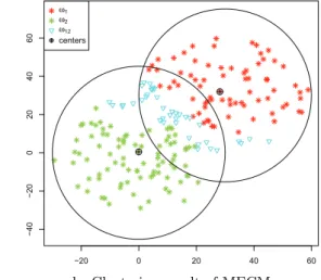
We start by generating 2× 100 points uniformly distributed in two overlapped circles with a same radius R = 30 but with different centers. The coordinates of the first circle’s center are (0, 0) while the coordinates of the other circle’s center are (30, 30). The data set is displayed in Fig. 2-a.
−20 0 20 40 60 −4 0 −2 0 0 2 0 4 0 6 0 ω1 ω2 −20 0 20 40 60 −4 0 −2 0 0 2 0 4 0 6 0 ω1 ω2 ω12 centers
a. Overlapped data b. Clustering result of MECM
Figure 2: Clustering of overlapped data set
In order to show the influence of parameters in MECM and ECM, different values of γ, α, η and δ have been tested for this data set. The figure Fig. 3-a displays the three evidential indices varying with γ (α is fixed to be 2) by MECM, while Fig. 3-b depicts the results of MECM with different α but a fixed γ = 0.4 (η and δ are set 0.7 and 50, respectively, in the tests). For fixed
α and γ, the results with different η and δ are shown in Fig. 3-c. The effect of α and δ on the
clusterings of ECM is illustrated in Fig. 3-e. As we can see, for both MECM and ECM, if we want to make more imprecise decisions to improve ER, parameter α can be decreased. In MECM, we can also reduce the value of parameter γ to accomplish the same purpose. Although both α and
γ have effect on imprecise clusters in MECM, the mechanisms they work are different. Parameter α tries to adjust the penalty degree to control the imprecise rates of the results. However, for γ,
the same aim could be got by regulating the uncertainty degree of imprecise classes. It can be seen from the figures, the effect of γ is more conspicuous than α. Moreover, although α may be set too high to obtain good clusterings, “good” partitions can also be got by adjusting γ in this case. For both MECM and ECM, the stable limiting values of evidential measures are around 0.7 and 0.8. Such values suggest the equivalence of the two methods to a certain extent. Parameter
η is used for discounting the distance between uncertain objects and specific clusters. As pointed
out in Fig. 3-c, if γ and α are well set, it has little effect on the final clusterings. The same is true in the case of δ which is applied to detect outliers. The effect of the different values of parameter
β is illustrated in Fig. 3-d. We can see that it has little influence on the final results as long as
it is larger than 1. As in FCM and ECM, for which it is a usual choice, we use β = 2 in all the following experiments.
The improvement of precision will bring about the decline of recall, as more data could not be clustered into specific classes. What we should do is to set parameters based on our own requirement to make a tradeoff between precision and recall. For instance, if we want to make a cautious decision in which EP is relatively high, we can reduce γ and α. Values of these parameters can be also learned from historical data if such data are available.
For the objects in the overlapped area, it is difficult to make a hard decision i.e. to decide about their specific groups. Thanks to the imprecise clusters, we can make a soft decision. As analysed before, the soft decision will improve the precision of total results and reduce the risk of misclassifications caused by simply partitioning the overlapped objects into specific class. However, too many imprecise decisions will decrease the recall value. Therefore, the ideal partition should
make a compromise between the two measures. Set α = 1.8, γ = 0.2, η = 0.7 and δ = 50, the “best” (with relatively high values on both precision and recall) clustering result by MECM is shown in Fig. 2-b. As we can see, most of the data in the overlapped area are partitioned into imprecise cluster ω12 , {ω1, ω2} by the application of MECM. We adjust the coordinates of the
center of the second circle to get overlapped data with different proportions (overlap rates), and the validity indices of the clustering results by different methods are illustrated in Fig. 4. For the application of MECM, MCM and MFCM, each algorithm is evoked 20 times with randomly selected initial prototypes for the same data set and the mean values of the evaluating indices are reported. The figure Fig. 4-d shows the average values of the indices by MECM (plus and minus one standard deviation) for 20 repeated experiments as a function of the overlap rates. As we can see the initial prototypes indeed have effects on the final results, especially when the overlap rates are high. Certainly, we can avoid the influence by repeating the algorithm many times. But this is too expensive for MECM. Therefore, we suggest to use the prototypes obtained in MFCM or MCM as the initial. In the following experiments, we will set the initial prototypes to be the ones got by MFCM.
As it can be seen, for different overlap rates, the classical measures such as precision, recall, and RI are almost the same for all the methods. This reflects that pignistic probabilities play a similar role as fuzzy membership. But we can see that for MECM, EP is significantly high, and the increasing of overlap rates has least effects on it compared with the other methods. Such effect can be attributed to the introduced imprecise clusters which enable us to make a compromise decision between hard ones. But as many points are clustered into imprecise classes, the evidential recall value is low.
Overall, this example reflects one of the superiority of MECM that it can detect overlapped clusters. The objects in the overlapped area could be clustered into imprecise classes by this approach. Other possible available information or special techniques could be utilised for these imprecise data when we have to make hard decisions. Moreover, partitions with different degree of imprecision can be got by adjusting the parameters of the algorithm based on our own requirement.
5.2. Classical data sets from Gaussian mixture model
In the second experiment, we test on a data set consisting of 3× 50 + 2 × 5 points generated from different Gaussian distributions. The first 3× 50 points are from Gaussian distributions
G(µk, Σk)(k = 1, 2, 3) with µ1=(0, 0)T, µ2= (40, 40)T, µ3= (80, 80)T (47) Σ1= Σ2= Σ3= ( 120 0 0 120 ) ,
and the last 2× 10 data are noisy points follow G(µk, Σk)(k = 4, 5) with
µ4=(−50, 90)T, µ5= (−10, 130)T (48) Σ4= Σ5= ( 80 0 0 80 ) .
MECM is applied with the following settings: α = 1, δ = 100, η = 0.7, while ECM has been tested using α = 1.7, δ = 100 (The appropriate parameters can be determined similarly as in the
first example). One can see from Figs. 5-b and 5-c , MCM and MFCM can partition most of the regular data in ω1, ω2and ω3into their correct clusters, but they could not detect the noisy points
correctly. These noisy data are simply grouped into a specific cluster by both approaches. As can be seen from Fig. 5-d, for the points located in the middle part of ω2, ECM could not find their
exact group and misclassify them into imprecise cluster ω13. In the figures ωij, {ωi, ωj} denotes imprecise clusters.
As mentioned before, imprecise classes in MECM can measure ignorance and uncertainty at the same time, and the degree of ignorance in meta clusters can be adjusted by γ. We can see that MECM does not detect many points in the overlapped area between two groups if γ is set to 0.6. In such a case the test objects are partitioned into imprecise clusters mainly because of our ignorance about their specific classes. These objects attributed to meta classes mainly belong to noisy data in ω4and ω5. The distance of these points to the prototypes of specific clusters is large (but not too
large or they could be regarded to be in the emptyset, see Fig. 5-e). Thus the distance between the prototype vectors is relatively small so that these specific clusters are indistinguishable. Decreasing
γ to be 0.2 would make imprecise class denoting more uncertainty, as it can be seen from Fig. 5-f,
where many points located in the margin of each group are clustered into imprecise classes. In such a case, meta classes rather reflect our uncertainty on the data objects’ specific cluster.
The table Tab. 2 lists the indices for evaluating the different methods. Bold entries in each column of this table (and also other tables in the following) indicate that the results are significant as the top performing algorithm(s) in terms of the corresponding evaluation index. We can see that the precision, recall and RI values for all approaches are similar except from those obtained for ECM which are significantly lower. As these classical measures are based on the associated pignistic probabilities for evidential clusterings, it seems that credal partitions can provide the same information as crisp and fuzzy ones. But from the same table, we can also see that the evidential measures EP and ERI obtained for MECM are higher (for hard partitions, the values of evidential measures equal to the corresponding classical ones) than the ones obtained for other methods. This fact confirms the accuracy of the specific decisions i.e. decisions clustering the objects into specific classes. The advantage can be attributed to the introduction of imprecise clusters, with which we do not have to partition the uncertain or unknown objects into a specific cluster. Consequently, it could reduce the risk of misclassification. However, although ECM also deals with imprecise clusters, the accuracy is not improved as much as in the case of applying MECM. As illustrated before in the case of ECM application, many objects of a specific cluster are partitioned into an irrelevant imprecise class and, as a result, the evidential precision value and ERI decrease as well.
Table 2: The clustering results for gaussian points by different methods. For each method, we generate 20 data sets with the same parameters and report the mean values of the evaluation indices for all the data sets.
Precision Recall RI EP ER ERI
MCM 0.7802 0.9570 0.9002 0.7802 0.9570 0.9002 MFCM 0.8616 0.9797 0.9484 0.8616 0.9797 0.9484 FCM 0.8644 0.9820 0.9500 0.8644 0.9820 0.9500 ECM 0.8215 0.9353 0.9222 0.9069 0.8436 0.9294 MECM (γ = 0.2) 0.8674 0.9855 0.9520 0.9993 0.7721 0.9336 MECM (γ = 0.6) 0.8662 0.9851 0.9515 0.9958 0.9586 0.9868
We also test on “Iris flower”, “cat cortex” and “protein” data sets [12, 17, 22]. The first is object data while the other two are relational data sets. Thus we compare our method with FCM
and ECM for the Iris data set, and with RECM and NRFCM (Non-Euclidean Relational Fuzzy Clustering Method [19]) for the last two data sets. The results are displayed in Fig. 6.
Presented results allow us to sum up the characteristics of MECM. Firstly, one can see that the behavior of MECM is similar to ECM for traditional data. Besides, credal partitions provided by MECM allow to recover the information of crisp and fuzzy partitions. Moreover, we are able to balance influence of our uncertainty and ignorance according to the actual needs. The examples utilised before deal with classical data sets. But the superiority of MECM makes it applicable in the case of data sets for which only dissimilarity measures are known e.g. social networks. Thus in the following experiments, we will use some graph data to illustrate the behaviour of the proposed method on the community detection problem in social networks. The dissimilarity index used here is the one brought forward by Zhou [49]. To have a fair comparison, in the following experiments, we also compare with three classical algorithms for community detection i.e. BGLL [4], LPA [36] and ZFCM (a fuzzy c-means based approach proposed by Zhang et al. [46]). The obtained community structures are compared with known performance measures, i.e., NMI (Normalized Mutual Information), VI (Variation of Information) and Modularity.
5.3. Artificial graphs and generated benchmarks
To show the performance of the algorithm in detecting communities in networks, we first apply the method to a sample network generated from Gaussian mixture model. This model has been used for testing community detection approaches by Liu and Liu [29].
The artificial graph is composed of 3× 50 nodes, n1, n2,· · · , n150, which are represented by
150 sample points, x1, x2,· · · , x150, in two-dimensional Euclidean space. There are 3× 50 points
generated from Gaussian distributions G(µk, Σk)(k = 1, 2, 3) with
µ1= (1.0,4.0)T, µ2= (2.5, 5.5)T, µ3= (0.5, 6.0)T (49) Σ1= Σ2= Σ3= ( 0.25 0 0 0.25 ) .
Then, the edges of the graph are generated by the following thresholding strategy: if|xi−xj| ≤ dist, we set an edge between node i and node j; Otherwise the two nodes are not directly connected. The graph is shown in Fig. 7-a (with dist = 0.8) and the dissimilarity matrix of the nodes is displayed in Fig. 7-b. From the figures we can see that there are three significant communities in the graph, and some nodes in the bordering of their groups seem to be in overlapped classes as they contact with members in different communities simultaneously.
The table Tab. 3 lists the indices for evaluating the results. It shows that MECM performs well as the evidential precision resulting from its application is high. MECM utilization also results in decreasing the probabilities of clustering failure thanks to the introduction of imprecise clusters. This makes the decision-making process more cautious and reasonable.
The algorithms are also compared by means of Lancichinetti et al. [28] benchmark (LFR) networks. The results of different methods in two kinds of LFR networks with 500 and 1000 nodes are displayed in Figs. 8–9 respectively. The parameter µ showed in the x-axis in the figures identifies whether the network has clear communities. When µ is small, the graph has well community structure. In such a case, almost all the methods perform well. But we can see that when µ is
Table 3: The results for Gaussian graph by different methods
Precision Recall RI EP ER ERI NMI VI Modularity MCM 0.9049 0.9110 0.9392 0.9049 0.9110 0.9392 0.8282 0.3769 0.6100 MFCM 0.9067 0.9099 0.9396 0.9067 0.9099 0.9396 0.8172 0.4013 0.6115 ZFCM 0.9202 0.9224 0.9482 0.9202 0.9224 0.9482 0.8386 0.3545 0.6118 MECM 0.9470 0.9472 0.9652 0.9789 0.6060 0.8661 0.8895 0.2428 0.6072 BGLL 0.9329 0.9347 0.9564 0.9329 0.9347 0.9564 0.8597 0.3081 0.6119 LPA 0.3289 1.0000 0.3289 0.3289 1.0000 0.3289 0.0000 1.0986 0.0000
large, the results by MECM have the largest values of precision. It means that the decisions which partition the nodes into a specific cluster are of great confidence. In terms of NMI, the results are similar to those by BGLL and LPA, but better than those of MCM and MFCM. This fact well explains that the hard or fuzzy partitions could be recovered when necessary.
5.4. Some real-world networks
A. Zachary’s karate club. The Zachary’s Karate Club data [45] is an undirected graph which consists of 34 vertices and 78 edges. The original graph and the dissimilarity of the nodes are shown in Fig. 10-a and 10-b respectively.
Let the parameters of MECM be α = 1.5, δ = 100, η = 0.9, γ = 0.6. The modularity functions by MECM, MCM, MFCM and ZFCM (Fig. 12-a) peak around c = 2 and c = 3. Let c = 2, all the methods can detect the two communities exactly. If we set c = 3, a small community, which can also be found in the dissimilarity matrix (Fig. 10-b), is separated from ω1 by all the approaches
(see Fig. 11). But ZFCM assigns the maximum membership to ω1for node 9, which is actually in
ω2. It seems that the loss of accuracy in the mapping process may cause such results.
MECM does not find imprecise groups when γ = 0.6 as the network has apparent community structure, and this reflects the fact that the communities are distinguishable for all the nodes. But there may be some overlap between two communities. The nodes in the overlapped cluster can be detected by decreasing γ (increasing the uncertainty for imprecise communities). As is displayed in Fig. 11-c and d, by declining γ to 0.1 and 0.05 respectively (the other parameters remain unchanged), nodes 3 and 9 are clustered into both ω1 and ω2 (ω12) one after another.
From the results we can see that MECM takes both the ignorance and the uncertainty into consideration while introducing imprecise communities. The degree of ignorance and uncertainty could be balanced through adjusting γ. The analysis shows that there appears only uncertainty without ignorance in the original club network. In order to show the performance of MECM when there are noisy conditions such that some communities are indistinguishable, two noisy nodes are added to the original graph in the next experiment.
B. Karate club network with some added noisy nodes. In this test, two noisy nodes are added to the original karate club network (see Fig.13-a). The first one is node 35, which is directly connected with nodes 18 and 27. The other one is 36, which is connected to nodes 1 and 33. It can be seen from the dissimilarity matrix that node 36 has stronger relationships with both communities than node 35. This is due to the fact that the nodes connected to node 36 play leader roles in their own group, but node 35 contacts with two marginal nodes with “small” or insignificant roles in their own group only.
The results obtained by the application of different methods are shown in Fig. 14. The MECM parameters are set as follows: α = 1.5, δ = 100, η = 0.9 and γ is tuned according to the the extent that the imprecise communities reflect our ignorance. As we can see, MCM, MFCM and ZFCM simply group the two noisy nodes into ω1. With γ = 0.4 MECM regards node 36 as a member of
ω1while node 35 is grouped into imprecise community ω12. And ω12 mainly reflects our ignorance
rather than uncertainty on the actual community of node 36. This is why node 36 is not clustered into ω12since ω1and ω2are distinguishable for him but we are just not sure for the final decision.
The increase in the extent of uncertainty in imprecise communities results from the decrease of γ value. We can see that more nodes (including nodes 36,9,1,12,27, see Figs. 14-e and f) are clustered into ω12 or ω13 due to uncertainty. The imprecise communities consider both ignorance (node 35)
and uncertainty (other nodes).
These results reflect the difference between ignorance and uncertainty. As node 35 is only related to one outward node of each community, thus we are ignorant about which community it really belongs to. On the contrary, node 36 connects with the key members (playing an important role in the community), and in this case the dissimilarity between the prototypes of ω1 and ω2 is
relatively large so they are distinguishable. Thus there is uncertainty rather than ignorance about which community node 36 is in. In this network, node 36 is a “good” member for both communities, whereas node 35 is a “poor” member. It can be seen from Fig. 15-a that the fuzzy partition by MFCM also gives large similar membership values to ω1 and ω2 for node 35, just like in the case
of such good members as node 36 and 9. The obtained results show the problem of distinguishing between ignorance and the “equal evidence” (uncertainty) for fuzzy partitions. But Fig. 15-b shows that the credal partition by MECM assigns small mass belief to ω1 and ω2for node 35, indicating
our ignorance on its situation.
We also test our method on four other real-world graphs: American football network, Dolphins network, Lesmis network and Political books network1. The measures applied to evaluate the performance of different methods are listed in Tab. 4–7. It can been seen from the tables, for all the graphs MECM application results in a community structure with high evidential precision level. The precision results from a cautious decision making process which clusters the noisy nodes into imprecise communities. In terms of classical performance measures like NMI, VI and modularity, MECM slightly outperforms the other algorithms. Note that these classical measures for hard partitions are calculated by the pignistic probabilities associated with the credal partitions provided by MECM. Therefore, we can also see the possibility to recover the hard decisions here when using the proposed evidential detection approach.
Table 4: The results for American football network by different methods
Precision Recall RI EP ER ERI NMI VI Modularity MCM 0.7416 0.8834 0.9661 0.7416 0.8834 0.9661 0.8637 0.6467 0.5862 MFCM 0.7583 0.8757 0.9678 0.7583 0.8757 0.9678 0.8715 0.6160 0.5745 ZFCM 0.8176 0.9082 0.9765 0.8176 0.9082 0.9765 0.9035 0.4653 0.6022 MECM 0.8232 0.9082 0.9771 0.9303 0.8681 0.9843 0.9042 0.4625 0.5995 BGLL 0.7512 0.9120 0.9689 0.7512 0.9120 0.9689 0.8903 0.5195 0.6046 LPA 0.6698 0.8298 0.9538 0.6698 0.8298 0.9538 0.8623 0.6580 0.5757 5.5. Discussion
We will discuss for which application MECM is designed here. As analysed before, for MECM only dissimilarities between objects are required and only the intuitive assumptions need to be satisfied for the dissimilarity measure. Therefore, the algorithm could be appropriate for many clustering tasks for non-metric data objects. This type of data is very common in social sciences,