HAL Id: hal-01577934
https://hal.archives-ouvertes.fr/hal-01577934
Submitted on 28 Aug 2017
HAL is a multi-disciplinary open access
archive for the deposit and dissemination of
sci-L’archive ouverte pluridisciplinaire HAL, est destinée au dépôt et à la diffusion de documents
Robin Bouclier, Jean-Charles Passieux, Michel Salaün
To cite this version:
Robin Bouclier, Jean-Charles Passieux, Michel Salaün. Development of a new, more regular, mortar method for the coupling of NURBS subdomains within a NURBS patch: Application to a non-intrusive local enrichment of NURBS patches. Computer Methods in Applied Mechanics and Engineering, Elsevier, 2017, 316, pp.123-150. �10.1016/j.cma.2016.05.037�. �hal-01577934�
6 7 8 9 10 11 12 13 14 15 16 17 18 19 20 21 22 23 24 25 26 27 28 29 30 31 32 33 34 35 36 37 38 39 40 41 42 43 44 45 46 47 48 49 50 51 52 53 54 55 56 57
Development of a new, more regular, mortar method for
the coupling of NURBS subdomains within a NURBS
patch: Application to the non-intrusive local enrichment
of NURBS patches
Robin Boucliera, Jean-Charles Passieuxb, Michel Sala¨unb
a Universit´e de Toulouse, INSA-Toulouse, IMT UMR CNRS 5219,
135 avenue de Rangueil, F-31077 Toulouse Cedex 04, France
bUniversit´e de Toulouse, INSA/UPS/ISAE/Mines Albi, ICA UMR CNRS 5312
3 rue Caroline Aigle, 31400 Toulouse, France
Abstract
In this work, we develop a mortar method for the coupling of NURBS sub-domains within a NURBS patch that keeps the benefit of using more regular functions. The idea is to use two Lagrange multipliers to match, across the coupling interface, the tractions coming from the discrete displacements in addition to the discrete displacements. It results in a strategy that is suit-able with the continuity of the physical solution: when the physical solution is sufficiently smooth, the strategy enables to represent a C1 behavior; but,
when only a C0 displacement is expected, no additional errors are introduced
since only the traction force is continuous and not the whole derivative fields. Lower stress jumps at the coupling interface can then be observed which allows for a better transition of the information. As an application, a
non-Email addresses: bouclier@insa-toulouse.fr (Robin Bouclier),
passieux@insa-toulouse.fr(Jean-Charles Passieux), michel.salaun@isae.fr
9 10 11 12 13 14 15 16 17 18 19 20 21 22 23 24 25 26 27 28 29 30 31 32 33 34 35 36 37 38 39 40 41 42 43 44 45 46 47 48 49 50 51 52 53 54 55 56 57
intrusive algorithm is also built for the proposed coupling method, which enables simple and flexible local enrichments of NURBS patches without loosing the interest of using more regular functions. A range of numerical examples in two-dimensional linear elasticity are carried out along with com-parisons with other published NURBS coupling techniques to demonstrate the performance of the proposed coupling and its interest when combined to a non-intrusive strategy.
Keywords: Isogeometric analysis, NURBS, Domain decomposition, Mortar method, Non-intrusive coupling, Non-conforming geometries
1. Introduction
The IsoGeometric Analysis (IGA), which was first introduced in Hughes et al. [1] and later developed in Cottrell et al. [2], relies on the use of the same functions for the finite element analysis as those used to build the geome-try of Computer-Aided Design (CAD) models. Thus, Lagrange polynomials are replaced by Non-Uniform-Rational-B-Splines (NURBS) functions, which constitute the most commonly used technology in CAD. This enables one to deal with both design and analysis using exactly the same geometric models. In addition to the geometric aspect, NURBS functions have a higher order of continuity, namely C(p−1) through the knot-span elements of the mesh for
a polynomial degree p, which on a per-degree-of-freedom basis exhibits in-creased accuracy in comparison to standard Finite Element Methods (FEM) (see, e.g., [3] for a theoretical analysis, [4] for structural vibrations, [5] for standard elasticity, [6] for embedded domain methods and [7, 8] for shell anal-ysis). If the global accuracy of NURBS is now proved, difficulties are still
9 10 11 12 13 14 15 16 17 18 19 20 21 22 23 24 25 26 27 28 29 30 31 32 33 34 35 36 37 38 39 40 41 42 43 44 45 46 47 48 49 50 51 52 53 54 55 56 57
encountered to integrate different discrete models in a NURBS patch. The reason for this is the rigid tensor product structure of NURBS which neces-sarily implies a structured quadrangular mesh. As a consequence, the local mesh refinement is not possible directly with the NURBS technology. More generally, the delimitation of a subregion of any shape within a NURBS patch is far from trivial, which prevents from the simple modeling of any specific local behaviors (e.g., introduction of an inclusion [9], crack propaga-tion [11, 10], emergence of a plastic zone [12], ...). Indeed, the basic strategy may involve a re-parametrization of the whole NURBS model, including the splitting of the new geometry into several patches with C0 continuity at the
boundaries. This entails a considerable modeling effort which is often as com-plex and time consuming as standard mesh generation and then, is opposed to the core idea of IGA.
To answer the issue of local mesh refinement, numerous research works have been dedicated to the construction of new splines these last years. To start with, one may cite the hierarchical B-splines and NURBS [13, 14, 15]. These new splines are easy to implement but the local mesh refinement still seems to spread for higher-order functions. With similar properties, one may also cite the development of LRB-splines [16] and multigrids-based NURBS [20]. Alternatively, another technology seems to have gathered an important momentum from both the computational geometry and analy-sis communities : the so-called T-splines [17, 18, 19]. In addition to be efficient for local mesh refinement, the T-splines also appear suitable to ad-dress trimmed multi-patch geometries. However, the implementation can appear complex and additional efforts may be necessary for the more general
9 10 11 12 13 14 15 16 17 18 19 20 21 22 23 24 25 26 27 28 29 30 31 32 33 34 35 36 37 38 39 40 41 42 43 44 45 46 47 48 49 50 51 52 53 54 55 56 57
situations mentioned above (modeling of an inclusion, local fracture, local plasticity).
To circumvent the problem, the purpose of this work is to develop a cou-pling method that is able to connect different NURBS subdomains within a global NURBS patch. Regarding NURBS coupling, many attempts have been devoted these last five years to the connection of NURBS patches to foster the study of multi-patch geometries. Certainly one of the first works on the subject was that of Hesch and Betsch [21], who used a Lagrange multiplier field to add the work performed by coupling tractions along the interface to the weak form. In the framework of NURBS Lagrange multiplier methods, one may also cite the work of Brivadis et al. [22] where several choices of Lagrange multiplier spaces are investigated theoretically and nu-merically. Then, a comparative numerical study in Apostolatos et al. [23] showed the efficiency of a Nitsche-based technique for NURBS. Nitsche cou-pling has subsequently been used for connecting 3D NURBS patches [9], for 3D-plate NURBS coupling [24, 25], and with NURBS immersed boundary methods [26]. Even if it may appear interesting due to the absence of ad-ditional degrees of freedom, the Nitsche method leads to a comparatively high computational effort since an additional eigenvalue problem has to be solved for the stabilizing term. As a result, Dornisch et al. [27] developed a weak substitution method to simplify the implementation and reduce the computational cost. From this overview, it may be noticed that most of the coupling techniques elaborated for NURBS nowadays are dedicated to the connection of NURBS patches, i.e., the coupling along a C0interface. Unlike
9 10 11 12 13 14 15 16 17 18 19 20 21 22 23 24 25 26 27 28 29 30 31 32 33 34 35 36 37 38 39 40 41 42 43 44 45 46 47 48 49 50 51 52 53 54 55 56 57
NURBS subdomains within a NURBS patch, i.e., where the continuity of the basis functions is expected to be higher than C0. As a result, the objective of
our work is to develop a coupling formulation that makes use of the higher-order continuity achieved by the NURBS functions. In particular, the better representation of the derivative fields offered by NURBS is of importance.
When applied to perform local enrichment, an interesting feature of a coupling method may be its ability to be implemented using a non-intrusive strategy. Roughly speaking, a method is said to be non-intrusive when its implementation is very simple from existing techniques and numerical codes. In the context of standard FEM, a group of global/local coupling methods, classified as non-intrusive, has emerged these last years. Based on the idea of Whitcomb [28] and formalized later in Gendre et al. [12] for the modeling of local plasticity, these methods involve the definition of two finite element models: a global coarse model of the whole structure and a local more de-tailed ”submodel” meant to replace the global model in the area of interest. An iterative coupling technique is used to perform the substitution in an exact but non-intrusive way: only interface data are transmitted from one model to the other and the global stiffness operator remains unchanged (in-dependently from the shape of the local domain). The performance of such a strategy has been highlighted in many applications (see, e.g., [11] for the modeling of crack propagation, [29] for the modeling of localized uncertain-ties, [30] for 3D-plate coupling and [31] for nonlinear domain decomposition). More recently, an extension in the NURBS context has been proposed in Bouclier et al. [32] and has proved to be a good candidate for NURBS local enrichment. Among the advantages, one may cite the elimination of costly
9 10 11 12 13 14 15 16 17 18 19 20 21 22 23 24 25 26 27 28 29 30 31 32 33 34 35 36 37 38 39 40 41 42 43 44 45 46 47 48 49 50 51 52 53 54 55 56 57
NURBS re-parametrization procedures for the global model (even if the lo-cal area evolves), the possibility to assemble and factorize the global stiffness operator only once, the good conditioning of the systems to be solved, and the easy merging for a NURBS code with any other specific numerical codes. However, the coupling method used in this contribution was the classical one and thus, only a C0 continuity across the coupling interface was ensured. As
a result, the goal of the present work is not only to develop a coupling method suitable with the higher-order continuity of NURBS, but also to be able to implement it in a non-intrusive way to perform NURBS local enrichment.
In this context, we propose in this paper a coupling method in which the tractions coming from the discrete displacements are matched, in addition to the usual discrete displacements, across the coupling interface. It results in a strategy able to represent a C1 behavior at the interface but also suitable to
capture a C0 displacement (such as in the case of bi-material structures for
example). The reason for this is that only physical quantities are transmitted from one model to the other. To meet the non-intrusive aspect, a Lagrange multiplier approach is followed. More precisely, two Lagrange multipliers are introduced to ensure the two coupling constraints. We believe that the proposed method is more consistent with the analysis properties of IGA since it allows for a smoother representation of the solution across the coupling interface.
The paper is organized as follows: first a brief review of IGA with NURBS is given and the reference coupling problem to be solved is presented in Section 2; after reviewing the classical NURBS approaches, the new cou-pling method is constructed in Section 3; then, the associated iterative
9 10 11 12 13 14 15 16 17 18 19 20 21 22 23 24 25 26 27 28 29 30 31 32 33 34 35 36 37 38 39 40 41 42 43 44 45 46 47 48 49 50 51 52 53 54 55 56 57
intrusive algorithm is built in Section 4; Section 5 presents a set of numerical experiments in two-dimensional linear elasticity to assess the performance of our methodology; finally, concluding remarks are formulated in section 6. 2. The reference NURBS domain decomposition problem
This section establishes the context of the study and introduces the cor-responding notations. First, a brief review of the concept of NURBS-based IGA is provided and the difficulty to integrate different discrete models in different regions of a NURBS patch is highlighted. Then, the reference do-main decomposition problem along with its governing equations and its weak form is presented.
2.1. Isogeometric analysis based on NURBS
For the discretization of the problem, the recent concept of IGA based on NURBS functions is used. Let us start by briefly reviewing the concept. Only the fundamentals are given here. For further details, the interested reader is referred to the references cited below.
The NURBS concept was first introduced in Hughes et al. [1] and formal-ized more recently in the book by Cottrell et al. [2]. NURBS functions are a generalized version of B-spline functions and have become a standard for geometric modeling in CAD and computer graphics (see, for example, Cohen et al. [33], Piegl and Tiller [34], Farin [35] and Rogers [36]). These functions lend themselves to an exact representation of many shapes used in engineer-ing, such as conical sections. They can be viewed as rational projections of higher-order B-splines and, therefore, they possess many of the properties of B-splines, the most interesting one being their high degree of continuity.
9 10 11 12 13 14 15 16 17 18 19 20 21 22 23 24 25 26 27 28 29 30 31 32 33 34 35 36 37 38 39 40 41 42 43 44 45 46 47 48 49 50 51 52 53 54 55 56 57
For the presentation in this section, we consider a domain in 3D so as to be general. If NA, A ∈ {1, 2, .., n} denote the n 3D NURBS functions,
ωA, A ∈ {1, 2, .., n} the associated weights and PA, A ∈ {1, 2, .., n} the
asso-ciated control points of coordinates xA in the global coordinate system, the
geometry of the structure is described through the position vector M defined as: M = n � A=1 NAxA, (1)
where the NURBS functions are obtained from the B-spline functions NA, A ∈
{1, 2, .., n} such that: NA = NAwA �n A=1NAwA . (2)
Now, all one needs to do in order to define the 3D B-spline functions NA
at control point PA is to perform the tensor product of the 1D B-spline
functions associated with this point in the three spatial directions. If one denotes M1
i, i ∈ {1, 2, .., n1}, Mj2, j ∈ {1, 2, .., n2} and Mk3, k ∈ {1, 2, .., n3}
the n1, n2 and n3 1D B-spline functions associated with each of the three
spatial directions, this means that at control point PA, which corresponds to
the ith, jth and kth control points in these directions, one has:
NA = Mi1× Mj2× Mk3. (3)
The 1D B-spline functions are defined using a knot vector. Each knot vector associated with a direction is defined in the parametric domain. For example, for the first direction, one takes knot vector Ξ = {ξ1, ξ2, .., ξn1+p+1}, where
9 10 11 12 13 14 15 16 17 18 19 20 21 22 23 24 25 26 27 28 29 30 31 32 33 34 35 36 37 38 39 40 41 42 43 44 45 46 47 48 49 50 51 52 53 54 55 56 57
and p the polynomial degree of the functions M1
i, i ∈ {1, 2, .., n1}. The
knots divide the parametric space into knot-span elements. In the following, the knot-span elements will be also simply denoted by the elements. The interval [ξ1, ξn1+p+1] constitutes the NURBS patch. Thus, unlike standard
FEM where each element has its own parametrization, the parametric space of B-Spline functions is localized onto the patch. The patch may be seen as a macro-element. Many geometries utilized for academic test cases can be modelled with a single patch. In two-dimensional topologies, a patch is a rectangle in the parametric domain. In three dimensions it is a cuboid.
There can be more than one knot at a given location of the parametric space. If m is the multiplicity of the considered knot, the functions have Cp−m continuity at that location. Thus, for quadratic and higher-order NURBS, the continuity at the elements boundaries at the interior of the NURBS patch is expected to be higher than the classical C0 regularity encountered
in standard FEM. If the knots are evenly spaced, the knot vector is said to be uniform. A knot vector whose first and last knots have multiplicity p + 1 is said to be open. In this case, the basis is interpolating at the boundary nodes of the interval, which facilitates the application of the boundary conditions. Only open uniform knot vectors will be considered in this work. The 1D B-spline basis functions for a given order p are defined recursively from the knot vector using the Cox-de Boor recursion formula (see, for example, Cohen et al. [33]). To take advantage of the superior approximation properties of NURBS functions, we choose them to be at least of polynomial degree two in the three spatial directions. As far as continuity is concerned, we perform k-refinement, meaning that we add elements while keeping the higher
9 10 11 12 13 14 15 16 17 18 19 20 21 22 23 24 25 26 27 28 29 30 31 32 33 34 35 36 37 38 39 40 41 42 43 44 45 46 47 48 49 50 51 52 53 54 55 56 57
degree of continuity of the NURBS functions, namely Cp−1 at the knot level. The positions of the control points and the values of the associated weights can be adjusted in order to build conical sections exactly, after which these geometries are preserved through mesh refinement. For a good overview of mesh generation and refinement, see Cottrell et al. [37].
The tensor product nature of NURBS shape functions (see Eq. (3)) makes it difficult to handle localized phenomena within the NURBS patch. In other words, we necessarily end up with a structured quadrangular mesh in a NURBS patch. For example, this makes the local mesh refinement impossible directly (see, e.g., [15] for completeness). More generally, this makes the integration of a subregion (of any shape) within a NURBS patch far from trivial. Indeed, since standard IGA technology requires a boundary fitted discretization for the analysis, a re-parametrization of the whole NURBS model taking into account the subregions may be required. This may lead to the splitting of the new geometry into several patches with C0 continuity at
the boundaries. This entails a considerable modelling effort, which is often as complex and time consuming as standard mesh generation. More details regarding this issue can be found in [26, 32].
2.2. The NURBS domain decomposition problem
To circumvent the problem of the integration of subregions within a NURBS patch, it is proposed in this work to develop a coupling method that is able to connect different NURBS subdomains within a global NURBS patch. The corresponding domain decomposition problem to be solved is introduced in the following.
9 10 11 12 13 14 15 16 17 18 19 20 21 22 23 24 25 26 27 28 29 30 31 32 33 34 35 36 37 38 39 40 41 42 43 44 45 46 47 48 49 50 51 52 53 54 55 56 57 2.2.1. Governing equations.
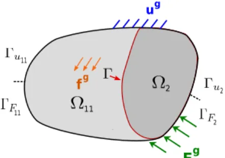
We consider in this work the case of multi-domain linear elasticity in Ω⊂ Rd, d = 2 or 3 being the dimension of the problem. Domain Ω constitutes
the NURBS patch to be decomposed into subdomains. For simplicity in the presentation, we assume that Ω is divided into only two disjoint, open and bounded subsets Ω11 and Ω2 such that Ω = Ω11 ∪ Ω2 and Ω11 ∩ Ω2 = ∅.
Those two non-overlapping subdomains share a common interface denoted Γ (see Fig. 1). Domains Ω11 and Ω2 are subjected to body forces f11g and f
g
2,
respectively. Furthermore, forces Fg11 and Fg2 are associated to boundaries ΓF11 and ΓF2 and, displacements u
g
11 and ug2 are prescribed over boundaries
Γu11 and Γu2. The boundaries satisfy the following relations :
ΓFm∪ Γum∪ Γ = ∂Ωm ΓFm∩ Γum =∅ ΓFm∩ Γ = ∅ Γum∩ Γ = ∅ with m = 11 and 2.
Remark 1. As subdomains are open, one would need to write Ω =
o
� �� � Ω11∪ Ω2
to be rigorous with the boundary Γ. In the paper, we decide to omit this notation for the sake of readability.
Remark 2. Regarding the notation, the reason why we use Ω11 and Ω2 for
the subdomains instead of Ω1 and Ω2 will appear in section 4.
Regarding the NURBS discretization, domains Ω11 and Ω2 are composed
9 10 11 12 13 14 15 16 17 18 19 20 21 22 23 24 25 26 27 28 29 30 31 32 33 34 35 36 37 38 39 40 41 42 43 44 45 46 47 48 49 50 51 52 53 54 55 56 57 ug Fg 11 fg 11 2 2 2 11
Figure 1: Reference domain decomposition problem.
practice, these regions are built by extracting a central zone from a larger NURBS patch made of open knot vectors (as it is done in hierarchical ap-proaches [13, 14, 15, 20]). The principle of such constructions is illustrated in Fig. 2 for the two-dimensional case. The figure shows the parametric spaces of three different domain decomposition problems. On these examples, we start by defining several discretizations of the global NURBS patch in Ω and then, we extract the regions that compose the subdomains. The associated one-dimensional case with quadratic B-Spline basis functions is added in Fig. 2(a). For each subdomain, the control points that are associated to the basis functions whose support is not in the subdomain are removed. We no-tice that an identical procedure is used in Chemin et al. [20] to construct the local NURBS grids of the multigrid algorithm. Depending on the NURBS discretization of the two subdomains along the interface Γ, three coupling situations are possible:
1. The coupling of matching meshes (see Fig. 2(a)): in this case, the inter-face Γ is aligned with the edges of the elements in the two subdomains and the meshes of the two subdomains along the interface are perfectly aligned.
9 10 11 12 13 14 15 16 17 18 19 20 21 22 23 24 25 26 27 28 29 30 31 32 33 34 35 36 37 38 39 40 41 42 43 44 45 46 47 48 49 50 51 52 53 54 55 56 57
2. The coupling of non-matching meshes (see Fig. 2(b)): in this case, the interface Γ is aligned with the edges of the elements in the two subdomains but the meshes of the two subdomains along the interface are not aligned.
3. The coupling of non-conforming geometries (see Fig. 2(c)): in this case, the interface Γ is not aligned with the edges of the elements which means that some knot-span elements are overlapped.
From such constructions, it results that the continuity of the basis functions of the two subdomains at the coupling interface Γ is higher than C0 (provided
quadratic (or higher-order) NURBS basis functions are used). This is in contrast with the more usual situation of the coupling of IGA patches which is achieved along C0 interfaces (see, e.g., [9, 22, 23, 26, 27]).
Remark 3. Starting with the whole global NURBS patch and then extract-ing the discretizations of the subdomains as illustrated in Fig. 2 may not be necessary in practice. Indeed, to ensure a higher-order continuity of the func-tions at the coupling interface, only a few additional knot-span elements have to be considered at the exterior of the interface coupling. For example, in the case of conforming geometries (see Fig. 2(a) and 2(b)), only p additional knot-span elements are required to reach a Cp−1 continuity at the interface.
Remark 4. Regarding local mesh refinement, it may be noted from the three coupling cases presented above that we undertake to solve more general situ-ations than the ones classically encountered with hierarchical B-Splines and NURBS. Indeed, the usual IGA hierarchical approaches are often restricted to the situation of conforming geometries.
9 10 11 12 13 14 15 16 17 18 19 20 21 22 23 24 25 26 27 28 29 30 31 32 33 34 35 36 37 38 39 40 41 42 43 44 45 46 47 48 49 50 51 52 53 54 55 56 57 + Extraction Extraction
(a) Coupling of matching meshes.
+
Extraction Extraction
(b) Coupling of non-matching meshes.
+
Extraction Extraction
9 10 11 12 13 14 15 16 17 18 19 20 21 22 23 24 25 26 27 28 29 30 31 32 33 34 35 36 37 38 39 40 41 42 43 44 45 46 47 48 49 50 51 52 53 54 55 56 57
The problem to be solved is a classical two-domain linear elastic problem in Ω11 ∪ Ω2. In each subdomain, the kinematic constraints, the equilibrium
equations and the constitutive relations have to be verified. Using the sub-script m to denote a quantity that is valid over region Ωm, with m = 11 and
2, the corresponding governing equations read: um = ugm over Γum ; div(σm) + fmg = 0 in Ωm ; σm nm = Fgm over ΓFm ; σm = Cm ε (um) in Ωm. (4)
For the sake of readability, we decided to use bold symbols for vectors while we underline twice the second- and four times the fourth-order tensors. In the above equations, ε (um) denotes the infinitesimal strain tensors, σm the
Cauchy stress tensors and Cm the Hooke tensors. n11 and n2 represent the
outward unit normals to Ω11 and Ω2, respectively. For the coupling interface,
the continuity of the displacements:
u11− u2= 0 on Γ ; (5)
and the equilibrium of the traction forces:
σ11n11+ σ2n2 = 0 on Γ ; (6)
have to be ensured. In the following, we will consider the unit normal vector n over the interface Γ such that n = n11|Γ= −n2|Γ.
9 10 11 12 13 14 15 16 17 18 19 20 21 22 23 24 25 26 27 28 29 30 31 32 33 34 35 36 37 38 39 40 41 42 43 44 45 46 47 48 49 50 51 52 53 54 55 56 57
2.2.2. Weak form of the problem.
Let us introduce the subspaces of [H1(Ω)]d needed for the weak
equilib-rium of the complete domain Ω, namely: U =�u∈�H1(Ω)�d, u| Γu11 = ug11 and u|Γu2 = ug2 � ; V =�v ∈�H1(Ω)�d, v|Γv11 = 0 and v|Γu2 = 0 � . (7)
Using the principle of virtual work, we obtain the variational form of the elasticity problem (4)-(6), as follows:
Find u∈ U such that: a (u, v) = l (v) , ∀v ∈ V,
(8)
where the bilinear form a and the linear form l read: a (u, v) = � m=11,2 am(um, vm) = � m=11,2 � Ωm ε (vm) : Cm ε (um) dΩm ; l (v) = � m=11,2 lm(vm) = � m=11,2 � Ωm vm· fmgdΩm+ � ΓFm vm· FgmdΓFm. (9)
3. The proposed coupling method
In this part, the proposed coupling method is presented first under its variational continuum form and then under its discrete form. For a better understanding of the new method, we first recall in the variational setting two strategies that have been classically used in IGA: the mortar coupling (see, e.g., [22, 23]) and the Nitsche coupling (see, e.g., [23, 9, 24, 26, 25]). To avoid confusion with the newly developed method, we denote these estab-lished strategies by the ”classical mortar coupling” and the ”classical Nitsche
9 10 11 12 13 14 15 16 17 18 19 20 21 22 23 24 25 26 27 28 29 30 31 32 33 34 35 36 37 38 39 40 41 42 43 44 45 46 47 48 49 50 51 52 53 54 55 56 57 coupling”, respectively. 3.1. The continuum version
We now regard the coupling problem (4)-(6) as a two-domain elasticity problem with mutually influencing boundary conditions along the common coupling interface Γ. We thus start by defining the functional spaces Um
and Vm over domain Ωm that will contain the solution and trial functions
respectively: Um = � um ∈ � H1(Ωm) �d , um|Γum = u g m � ; Vm= � vm∈ � H1(Ωm) �d , vm|Γum = 0 � . (10)
We recall that the subscript m∈ {11, 2} denotes a quantity that is valid over domain Ωm.
3.1.1. A review of the classical mortar approach.
In the context of mortar approaches or, in other words, in the context of Lagrange multiplier methods, a mixed formulation is set up to impose the coupling constraints (5) and (6). Classically, a single Lagrange multiplier λ∈ M (where M is an appropriate space) is introduced, as the dual unknown, to represent both of the interface traction forces, i.e., σ11n = σ2n = −λ in
Eq. (6). Then, the interface Dirichlet condition (5) is imposed in a weak sense over Γ using the Lagrange multiplier. This leads to the formulation of the following Lagrangian of the coupled problem:
Lbasic � (u11, u2), λ � = 1 2a11(u11, u11)+ 1 2a2(u2, u2)−l11(u11)−l2(u2)+b (λ, u11− u2) . (11)
9 10 11 12 13 14 15 16 17 18 19 20 21 22 23 24 25 26 27 28 29 30 31 32 33 34 35 36 37 38 39 40 41 42 43 44 45 46 47 48 49 50 51 52 53 54 55 56 57
Bilinear forms am and linear forms lm are given in Eq. (9) and bilinear form
b is defined such that:
b (µ, u) = �
Γ
µ· udΓ. (12)
With above developments, we can finally obtain the classical mortar coupling formulation of the reference problem as follows:
Find u11 ∈ U11, u2 ∈ U2, and λ∈ M such that:
a11(u11, v11) + b(λ, v11) = l11(v11) , ∀v11 ∈ V11 ; a2(u2, v2)− b(λ, v2) = l2(v2) , ∀v2 ∈ V2 ; b(µ, u11− u2) = 0, ∀µ ∈ M. (13)
One advantage of such a formalism is that within its discrete form, it enables to keep separated and unmodified the stiffness operators associated to the subdomains. Indeed, the communication between the subdomains is performed via the Lagrange multiplier only. This feature is the basis of the non-overlapping domain decomposition methods developed for high performance computing on parallel computer architectures (see, e.g., [38, 39, 40]). In the same idea, such a property enables to build non-intrusive coupling algorithms for the modeling of local behaviors (see, e.g., [12, 11, 30, 31, 32]). Several numerical codes can then be coupled in an iterative way with the exchange of only interface data to carry out the global/local simulation. However, the drawback of such a formulation is that a special care may be required for the construction of the approximation space of M to avoid undesirable energy-free oscillations (due to the non-satisfaction of the inf-sup condition).
9 10 11 12 13 14 15 16 17 18 19 20 21 22 23 24 25 26 27 28 29 30 31 32 33 34 35 36 37 38 39 40 41 42 43 44 45 46 47 48 49 50 51 52 53 54 55 56 57
3.1.2. A review of the classical Nitsche approach.
Conversely, in the Nitsche coupling technique, the stiffness operators of the different subdomains are merged together which eliminates the need of additional degrees of freedom. A connection between Nitsche and Lagrange multiplier couplings can be made (see, e.g., [41, 42]). Starting with the Lagrange multiplier method, the idea to obtain the Nitsche method is to replace the Lagrange multiplier by the mean interface resultant force coming from the displacement. We therefore define the average of the stresses and of the virtual stresses on the interface as follows:
� σ�=�γσ11(u11) + (1− γ)σ2(u2) � |Γ= � γC11 ε (u11) + (1− γ)C2 ε (u2) � |Γ � τ�=�γσ11(v11) + (1− γ)σ2(v2) � |Γ= � γC11 ε (v11) + (1− γ)C2 ε (v2) � |Γ with γ ∈ [0, 1] . (14) We note that in most situations (particularly when the material properties of the subdomains to couple are close), γ = 1/2 is considered. Denoting now the jump of the displacements and of the virtual displacements on the interface such as:
9 10 11 12 13 14 15 16 17 18 19 20 21 22 23 24 25 26 27 28 29 30 31 32 33 34 35 36 37 38 39 40 41 42 43 44 45 46 47 48 49 50 51 52 53 54 55 56 57
we obtain the following Nitsche bilinear form: aN � (u11, u2) , (v11, v2) � = a11(u11, v11) + a2(u2, v2)− � Γ�u� · � τ�ndΓ− � Γ � σ�n· �v�dΓ. (16)
This bilinear form needs finally to be enriched with a stabilization term to ensure the ellipticity of the boundary value problem. Denoting the stabiliza-tion parameter by α, the stabilized variastabiliza-tional formulastabiliza-tion of the problem using the classical Nitsche approach can be written as follows:
Find (u11, u2)∈ U11× U2, such that:
aN � (u11, u2) , (v11, v2) � + α � Γ�u� · �v�dΓ = l 11(v11) + l2(v2) , ∀ (v11, v2)∈ V11× V2. (17) While in formulation (13) a suitable approximation space for the Lagrange multiplier needs to be chosen, the Nitsche approach (17) requires the choice of a suitable value for α. It has been shown that an estimation of α can be obtained by solving a generalized eigenvalue problem [23, 9] (or several local eigenvalue problems [26]) over the interface.
3.1.3. The newly-developed mortar approach.
In the two coupling formulations presented above, we notice that the prop-erty of higher-order continuity of the NURBS basis functions at the interface Γ has not been used. Indeed, if the continuity of the discrete displacement is enforced across Γ, there is no reason with such formulations that the in-terface traction force coming from the discrete displacement is continuous through the interface. In other words, there is no reason that the discrete
9 10 11 12 13 14 15 16 17 18 19 20 21 22 23 24 25 26 27 28 29 30 31 32 33 34 35 36 37 38 39 40 41 42 43 44 45 46 47 48 49 50 51 52 53 54 55 56 57
displacement solution satisfies: � σ11(u11)n− σ2(u2)n � |Γ= � C11 ε(u11)n− C2 ε(u2)n � |Γ = 0. (18)
However, it has to be noted that such an equality is verified by a single NURBS patch solution and that such a constraint seems to have a physical meaning according to Eq. (6) of our reference problem. As result, we propose in this work to add constraint (18) in our solution spaceU and virtual space V (see, eq. (7)). We emphasize that such a treatment seems to be consis-tent here because the interpolated functions are more regular (at least C1),
which implies that the gradients of the displacement, and so the stresses and tractions forces, are defined at the coupling interface.
To take into account the additional constraint in our coupling formula-tion, we propose to follow a Lagrange multiplier strategy since the intended application of this work is the non-intrusive local enrichment of NURBS patches. Two Lagrange multipliers are thus introduced: λu∈ Mu is devoted
to the displacement relation as in the classical approach and λσ ∈ Mσ is
devoted to the constraint (18). The associated new Lagrangian reads: Lnew � (u11, u2), (λu, λσ) � = 1 2a11(u11, u11) + 1 2a2(u2, u2)− l11(u11)− l2(u2) + b (λu, u11− u2) + b�λσ, σ11(u11)n− σ2(u2)n � , (19)
9 10 11 12 13 14 15 16 17 18 19 20 21 22 23 24 25 26 27 28 29 30 31 32 33 34 35 36 37 38 39 40 41 42 43 44 45 46 47 48 49 50 51 52 53 54 55 56 57
which enables to get the following variational formulation:
Find u11 ∈ U11, u2∈ U2, λu∈ Mu and λσ ∈ Mσ such that:
a11(u11, v11) + b(λu, v11) + b(λσ, σ11(u11)n) = l11(v11) , ∀v11 ∈ V11 ; a2(u2, v2)− b(λu, v2)− b(λσ, σ2(u2)n) = l2(v2) , ∀v2 ∈ V2 ; b(µu, u11− u2) = 0, ∀µu ∈ Mu ; b(µσ, σ11(u11)n− σ2(u2)n) = 0, ∀µσ ∈ Mσ. (20) This formulation will be denoted ”new mortar coupling” in the following of the paper. We will show in section 5 (Numerical results) that the addition of constraint (18) for the coupling enables to represent a C1 displacement
across the interface while only a C0 solution can be described in the
clas-sical approaches. Furthermore, we insist on the fact that the additional constraint considered has a physical meaning from the reference coupling problem. Thus, the new coupling is also suited to describe a solution that is not C1 across the interface (such as in the case of the coupling of
differ-ent materials for instance). When the intended solution is not C1, we will
see that no additional errors are introduced since only the interface traction force coming from the discrete displacement is continuous (and not the whole derivative fields of the discrete displacement).
3.2. The discrete version
We now construct the discrete operators associated to the new mortar coupling formulation. To this end, let us introduce the NURBS functions N11
9 10 11 12 13 14 15 16 17 18 19 20 21 22 23 24 25 26 27 28 29 30 31 32 33 34 35 36 37 38 39 40 41 42 43 44 45 46 47 48 49 50 51 52 53 54 55 56 57
and Ω2, respectively. Following the principle of isoparametric elements, the
basis (N11
A )A∈{1,2,..,n11} and (N
2
B)B∈{1,2,..,n2} are used to build the finite
ele-ment spaces Uh
11 and U2h corresponding to the discretization of U11 and U2,
respectively. As stated above, the discretization of spacesMu and Mσ may
require special attention to avoid numerical problems. Nevertheless, we have been able to obtain satisfactory results (i.e., that we never encountered in-stabilities in our computations) with a very basic strategy. For the sake of simplicity, we chose to use the same finite element space Mh for the two
Lagrange multipliers. Then, we adopted a classical strategy (see, e.g., [31]): the trace along the coupling interface Γ of the NURBS functions of subdo-main Ω2 (assumed to be descretized with the finer mesh) was considered for
Mh. The resulting one-dimensional functions are denoted �Nλ D
�
D∈{1,2,..,nλ}.
We emphasize that other choices could also have been made: for instance, the trace of the NURBS functions of domains Ω1 along the coupling interface
seems to produce equivalent results. By substituting the NURBS approxi-mations in the weak form Eq. (20), we can obtain the following linear system to be solved: [K11] [0] [LA11]T [DA11]T [0] [K2] − [LA2]T − [DA2]T [LA11] − [LA2] [0] [0] [DA11] − [DA2] [0] [0] {U11} {U2} {Λu} {Λσ} = {F11} {F2} {0} {0} . (21) Operators [K11] (respectively {F11}) and [K2] (resp. {F2}) are the classical
stiffness matrices (resp. vector forces) associated to domains Ω11 and Ω2.
9 10 11 12 13 14 15 16 17 18 19 20 21 22 23 24 25 26 27 28 29 30 31 32 33 34 35 36 37 38 39 40 41 42 43 44 45 46 47 48 49 50 51 52 53 54 55 56 57
[DA2] are the new mortar coupling operators that enable to enforce the equilibrium of the tractions coming from the discrete displacement along Γ. They are constructed as follows:
[LA11] = � Γ [Nλ]T[nn] [D11] [B11] dΓ ; [LA2] = � Γ [Nλ]T [nn] [D2] [B2] dΓ. (22) [B11] and [B2] are the standard strain-displacement matrices associated to
spaces Uh
11 and U2h, [Nλ] represents the standard shape function matrix of
Mh and [D
11] and [D2] constitute the discrete Hooke matrices. In addition,
matrix [nn] is introduced to perform the product between the stress ten-sor and the outward unit normal (see [9, 26] for more details regarding the construction of such operators).
Remark 5. Unlike the classical mortar approach, each of the two Lagrange multipliers alone does not have a physical meaning in the proposed formula-tion. Nevertheless, there exists a combination of the two Lagrange multipliers that can be interpreted as the reaction forces between the two subdomains. In-deed, considering for instance the first set of equations of system (21), we no-tice that the reaction forces{R11} along Γ of subdomain Ω11 can be expressed
as follows:
{R11} = ([K11] {U11} − {F11}) = − [LA1]T {Λu} − [DA1]T{Λσ} . (23)
Remark 6. Even if presented in the case of elastic constitutive laws, one may notice that the proposed coupling formulation holds for material non-linearities (such as elastoplasticity). Only additional implementation efforts
9 10 11 12 13 14 15 16 17 18 19 20 21 22 23 24 25 26 27 28 29 30 31 32 33 34 35 36 37 38 39 40 41 42 43 44 45 46 47 48 49 50 51 52 53 54 55 56 57
may be taken in this case due to the necessity of evaluating the discrete stress tensor along the coupling interface.
4. Application: development of the non-intrusive coupling strategy The coupling method developed above can be applied to any NURBS do-main decomposition problems (provided higher-order continuity is available at the interface). As an application, we build in this section a non-intrusive algorithm to perform the local enrichment of a NURBS patch with the new mortar coupling. The performance of a non-intrusive strategy for the model-ing of local behaviors in a NURBS patch has been demonstrated in Bouclier et al. [32]. The goal here is to combine the advantages of a non-intrusive strategy with the property of higher-order continuity of the newly-developed mortar coupling. Since the proposed coupling formulation is based on the use of Lagrange multipliers, the derivation of a non-intrusive strategy is rather straightforward. It is presented briefly in the following. For further details regarding the non-intrusive strategy, we encourage the interested reader to consult [32] and references cited therein.
4.1. The reference non-intrusive global/local problem
In this part, we consider that subdomain Ω2 represents a local region
where a refined model is required to correctly describe the local behavior of the NURBS patch. In the remaining zone of the NURBS patch (i.e., in Ω11), we assume that a coarser and simpler model is sufficient to represent
the global behavior of the solution. Rather than solving the system of equa-tions (21) directly (i.e., in a monolithic way), we proceed in an iterative way by involving a global model defined over the existing whole NURBS patch.
9 10 11 12 13 14 15 16 17 18 19 20 21 22 23 24 25 26 27 28 29 30 31 32 33 34 35 36 37 38 39 40 41 42 43 44 45 46 47 48 49 50 51 52 53 54 55 56 57
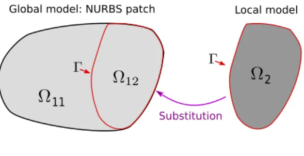
The situation is illustrated in Fig. 3. In order to do so, domain Ω12 is
intro-duced to characterize the region in which the global model of Ω11 is fictively
prolonged. Ω12 is defined in such a way that the NURBS patch domain is
recovered with Ω11∪ Ω12. From here on, we refer to domain Ω1 = Ω11∪ Ω12
to characterize the global NURBS patch that contains the global model ev-erywhere. The objective of the non-intrusive strategy is then to replace the global model over Ω12 by the local one in Ω2 without actually modifying the
global NURBS patch operators over Ω1.
Global model: NURBS patch Local model
Substitution 11
2
Figure 3: The non-intrusive global/local problem.
4.2. The non-intrusive global/local algorithm
Let us start by introducing the NURBS functions N1
C, C ∈ {1, 2, .., n1}
that discretize domain Ω1. As a consequence, the basis functions (NB11)B∈{1,2,..,n11}
constitute the restricted part of the basis (N1
C)C∈{1,2,..,n1} to domain Ω11. To
derive the non-intrusive strategy, we perform a continuous prolongation of the displacement solution from Ω11 to Ω12. We present the method in the
discrete case in the following.
We define{U1} the fictitious prolongation of {U11} to Ω1, so that{U1} |Ω11 =
9 10 11 12 13 14 15 16 17 18 19 20 21 22 23 24 25 26 27 28 29 30 31 32 33 34 35 36 37 38 39 40 41 42 43 44 45 46 47 48 49 50 51 52 53 54 55 56 57
{U12} (i.e., {U1} |Ω12 = {U12}). As well, we introduce the load vector
{F1} = {F11} + {F12} defined on Ω1. {F12} is constructed from body force
f12g and surface traction Fg12 that can be viewed as the fictitious prolonga-tion of f11g and Fg11 to Ω12. In practice, we take f12g = f
g 2 and F g 12 = F g 2.
Then, we make use of the additivity of the integral with respect to domain Ω1 = Ω11∪ Ω12, which gives us:
[K1]{U1} = [K11]{U1} + [K12]{U1} . (24)
[K1] and [K12] are the classical stiffness operators related to domains Ω1 and
Ω12. The equality (24) is used to modify the first part of the equations (21).
More precisely, this offers the possibility to split Eq. (21) into two parts: one for each domain Ω1 and Ω2. The solution of the coupled problem is finally
obtained through an iterative algorithm where the global and local models are computed alternatively. A standard fixed point can be implemented for that. For the nth iteration, we proceed as follows: starting with {U
1}(0),
{Λu}(0) and {Λσ}(0), we look for {U1}(n), {U2}(n), {Λu}(n) and {Λσ}(n) such
that:
1. Resolution of the full global problem:
[K1]{U1}(n) ={F1}−[LA1]T {Λu}(n−1)−[DA1]T{Λσ}(n−1)+[K12]{U1}(n−1).
9 10 11 12 13 14 15 16 17 18 19 20 21 22 23 24 25 26 27 28 29 30 31 32 33 34 35 36 37 38 39 40 41 42 43 44 45 46 47 48 49 50 51 52 53 54 55 56 57
2. Resolution of the local problem: [K2] − [LA2]T − [DA2]T − [LA2] [0] [0] − [DA2] [0] [0] {U2}(n) {Λu}(n) {Λσ}(n) = {F2} − [LA1] {U1}(n) − [DA1] {U1}(n) . (26) Thanks to the prolongation of the global model over Ω12, the whole stiffness
matrix of the global NURBS patch is now considered without any modifi-cation. During the iterations, only displacement and force exchanges at the interface Γ are required. In this sense, the strategy is said to be non-intrusive. In our case of a NURBS discretization, this may highly facilitate the model-ing of local behaviors since it avoids the complex task of constructmodel-ing a new NURBS parametrization of the global/local model (and of re-constructing it each time the local region evolves). In addition, it has to be noted that, regardless of the evolution of the shape of the local region, the global stiff-ness operator is assembled and factorized only once and the system (25) remains well-conditioned. The price to pay is the number of iterations but this one can be deeply reduced by means of accelerations techniques, such as based on an Aitken’s Delta Squared method or a Quasi-Newton method (see, e.g., [31, 32]). Numerical experiments to account for this last point will be carried out in section 5 (Numerical results).
Regarding the implementation, the convergence test usually used to stop this algorithm relies on the discrete reaction equilibrium between the two domains. In our case, the global reaction forces along Γ are defined as {R11} = ([K11] {U11} − {F11}) |Γ and have to be compared to the local
9 10 11 12 13 14 15 16 17 18 19 20 21 22 23 24 25 26 27 28 29 30 31 32 33 34 35 36 37 38 39 40 41 42 43 44 45 46 47 48 49 50 51 52 53 54 55 56 57
It leads to the following definition of the interface equilibrium residual:
η = � || {R11} + {R2} || || {F11} ||2+|| {F2} ||2
. (27)
Remark 7. It may be emphasized that we need to compute the reaction forces over Γ of the fictitious part of the global model ( i.e., [K12]{U1}) to
make the algorithm work. In order to do so, we use the simple strategy pro-posed in [32]: the quadrature rule coming from the local problem is transpro-posed within the global NURBS patch to estimate [K12]. We note that more
sophis-ticated strategies such as the ones elaborated for trimmed surfaces could have been used here (see, e.g., [43, 44, 45]). In the same idea, we need also to compute {R11} (involving [K11]) for the interface equilibrium residual (27).
The calculation is performed from the already computed stiffness [K12], i.e.:
[K11] = [K1]− [K12].
Remark 8. It may also be noted that the fictitious prolongation of the global solution over Ω12 ( i.e., {U12}) has no physical meaning (it depends on the
initialization) and has to be replaced by the solution {U2}.
5. Numerical examples
To assess the performance of the developed method, four numerical ex-amples are presented in this section. For each, a two-dimensional elastic model under plane stress is considered. The first two test cases are devoted to the study of the new coupling method presented in section 3 without the non-intrusive aspect: the resolution is performed in a monolithic way (i.e., the system of equations (21) is assembled and solved directly). In the
9 10 11 12 13 14 15 16 17 18 19 20 21 22 23 24 25 26 27 28 29 30 31 32 33 34 35 36 37 38 39 40 41 42 43 44 45 46 47 48 49 50 51 52 53 54 55 56 57
last two numerical problems, the iterative algorithm (25)-(26) of section 4 is implemented in view of performing the non-intrusive local enrichment of a NURBS patch. Unless otherwise stated, we consider quadratic NURBS basis functions with the maximum available continuity at the interior knots (i.e. C1). From here on, the mesh composed of N elements along the first length
and M elements along the second length will be denoted N × M. 5.1. Beam under shear load
5.1.1. Presentation and preliminary results.
The first example consists of a beam whose geometry and boundary con-ditions are given in Fig. 4. This problem has become popular in NURBS to evaluate a coupling method (see, e.g., [9, 24, 26]). The shear load at the right side is parabolic. As a result of the equilibrium of the structure, shear tractions of opposite signs and linearly varying normal tractions are found at the other side. A reference analytical solution is available for the problem in Zienckewich and Taylor [46]. For the coupling, we consider the situation of Fig. 4. The interface Γ is located at the middle of the structure. On this test case, we use the strategies illustrated in Figs. 2(a) and 2(b) to construct different matching and non-matching NURBS discretizations of the domain decomposition problem. We recall that this leads to basis functions of higher-order continuity at the interface Γ. A set of numerical experiments are carried out along with comparisons with classical published NURBS techniques on this test case to show the properties of the proposed coupling approach.
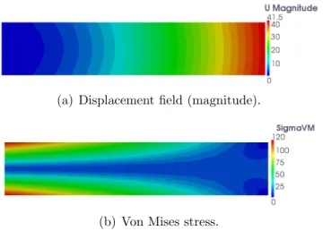
To start with, we plot in Fig. 5 the numerical solution in terms of displace-ment and von Mises stress for a two non-matching meshes model composed of 5 (along the x-direction) ×3 (along the y-direction) elements in Ω11 and
9 10 11 12 13 14 15 16 17 18 19 20 21 22 23 24 25 26 27 28 29 30 31 32 33 34 35 36 37 38 39 40 41 42 43 44 45 46 47 48 49 50 51 52 53 54 55 56 57 L c c x y
Figure 4: 2D solid beam under shear load: description and data of the problem.
5× 5 elements in Ω2. We consider Young moduli E11 = E2 = 1000 and
Poisson coefficients ν11 = ν2 = 0.3. The solution appears to be in a good
agreement with references [9, 26]. In particular, the transition of the solution from one model to the other appears very smooth.
(a) Displacement field (magnitude).
(b) Von Mises stress.
Figure 5: Solution obtained with the new mortar coupling for a two non-matching meshes
model (5× 3 and 5 × 5 knot-span elements in Ω11and Ω2, respectively).
5.1.2. Coupling of matching meshes.
To go further, we investigate more in details the transition across Γ of the component σxxof the stress tensor. Note that σxxis also the first component
9 10 11 12 13 14 15 16 17 18 19 20 21 22 23 24 25 26 27 28 29 30 31 32 33 34 35 36 37 38 39 40 41 42 43 44 45 46 47 48 49 50 51 52 53 54 55 56 57
across the coupling interface Γ according to Eq. (6). First, a two matching meshes model composed of 5× 4 elements in Ω11 and 5× 4 elements in Ω2 is
computed in Figs. 6 and 7. Here, we keep Young moduli E11 = E2 = 1000
and Poisson coefficients ν11 = ν2 = 0.3. More precisely, the distribution of
the exact error of the finite element model stress component σxxf e, i.e. the
error with respect to the reference analytical solution σxxex provided in [46]:
Err−Sig−xx =|σxxf e − σxxex|, (28)
is mapped around the interface in Fig. 6 (zoomed window: L/4 ≤ x ≤
3L/4 and −c ≤ y ≤ c). To better observe the behavior at the interface, the jump of σxx across Γ with respect to the vertical coordinate y is then
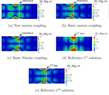
plotted in Fig. 7. For comparison purpose, the solutions provided by the basic mortar and basic Nitsche couplings are also computed and added to the graphs. For the Nitsche coupling, the stability factor was set to 20 as in [26]. Finally, reference C1 and C0 solutions are added to Fig. 6. The
reference C1 solution is the solution obtained by using a single quadratic C1
NURBS patch composed of 10×4 knot-span elements for the whole structure (associated knot vector such that {0 0 0 0.1 0.2 . . . 0.5 . . . 0.9 1 1 1} for the x-direction). For the reference C0 solution, the multiplicity of the middle
knot along x is increased in order to get a C0 continuity at the interface Γ
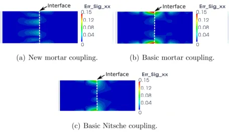
(knot vector{0 0 0 0.1 0.2 . . . 0.5 0.5 . . . 0.9 1 1 1} for the x-direction). We clearly observe that only the new mortar coupling is able to correctly represent the solution around the interface (see Fig. 6(a)). The error seems to vanish around the interface in this situation. For the classical couplings, error concentrations appear around the interface (see Figs. 6(b) and 6(c)).
9 10 11 12 13 14 15 16 17 18 19 20 21 22 23 24 25 26 27 28 29 30 31 32 33 34 35 36 37 38 39 40 41 42 43 44 45 46 47 48 49 50 51 52 53 54 55 56 57 Interface
(a) New mortar coupling.
Interface
(b) Basic mortar coupling.
Interface
(c) Basic Nitsche coupling.
C line1
(d) Reference C1 solution.
C line0
(e) Reference C0solution.
Figure 6: Distribution around the coupling interface of the exact error of the stress
com-ponent σxx for a two matching meshes model (4× 5 knot-span elements in Ω11 and Ω2)
and comparison with reference C1 and C0 solutions.
−10 −5 0 5 10 −0.4 −0.3 −0.2 −0.1 0 0.1 0.2 0.3 0.4 Jump of sig xx at the interface y New mortar coupling Basic mortar coupling Basic Nitsche coupling
9 10 11 12 13 14 15 16 17 18 19 20 21 22 23 24 25 26 27 28 29 30 31 32 33 34 35 36 37 38 39 40 41 42 43 44 45 46 47 48 49 50 51 52 53 54 55 56 57
By comparing the coupling solutions to the reference C1 and C0 solutions
(Figs. 6(d) and 6(e)), we notice that a C1 behavior across the interface can
be captured with the new mortar coupling while only a C0 solution at the
interface can be described in the classical approaches. Even if it is only observable for σxx in the presented figures, we emphasize that exactly the
same solutions (in terms of displacements, strains and stresses) are obtained for the new mortar coupling (Fig. 6(a)) as for the equivalent single C1 patch
(Fig. 6(d)). In this sense, our method can be classified as a C1 coupling
method: the whole derivative fields of the coupled solution are continuous across the interface. In the same idea, we can see in Fig. 7 that the jump across Γ of σxx is null here with the new coupling whereas it increases at the
exterior boundaries for the usual coupling techniques. Such a result accounts for the necessity of matching the interface tractions coming from the discrete displacement to get a better transition of the information and so, to obtain a better accuracy of the coupled solution.
5.1.3. Coupling at a bi-material interface.
To assess the performance of the proposed coupling method in situations where the solution is not C1 across the interface, the same numerical
experi-ment as in the previous section is carried out but with different constitutive materials for the subdomains. More precisely, we take E11 = 500 in Ω11 and
E2 = 1000 in Ω2 (and ν11 = ν2 = 0.3). Since the problem is isostatic, the
same reference solution in terms of stress as for the problem in [46] should be reached. Fig. 8 shows the distribution of the exact error of σxx around
the coupling interface. As in the previous part, the results of the new mortar coupling along with the classical couplings are given and reference C1 and
9 10 11 12 13 14 15 16 17 18 19 20 21 22 23 24 25 26 27 28 29 30 31 32 33 34 35 36 37 38 39 40 41 42 43 44 45 46 47 48 49 50 51 52 53 54 55 56 57
C0 solutions are also added. For the reference solutions, exactly the same
parametrizations as previously are taken but this time, E11 = 500 is applied
on the right part of the patch and E2 = 1000 is applied in the remaining
left area. For completeness, the evolution of the exact error regarding σxxat
each side of the interface with respect to the vertical coordinate y is plotted in Fig. 9. The jump of σxx across the coupling interface is not plotted for
this numerical experimentation since it can be observed in Fig. 9 with the discrepancy between the left and right interface errors.
Interface
(a) New mortar coupling.
Interface
(b) Basic mortar coupling.
Interface
(c) Basic Nitsche coupling.
C line1
(d) Reference C1 solution.
C line0
(e) Reference C0solution.
Figure 8: Distribution around the coupling interface of the exact error of the stress
compo-nent σxxfor the modeling of a bi-material structure with matching meshes (5×4 knot-span
elements in Ω11and Ω2) and comparison with reference C1 and C0 solutions.
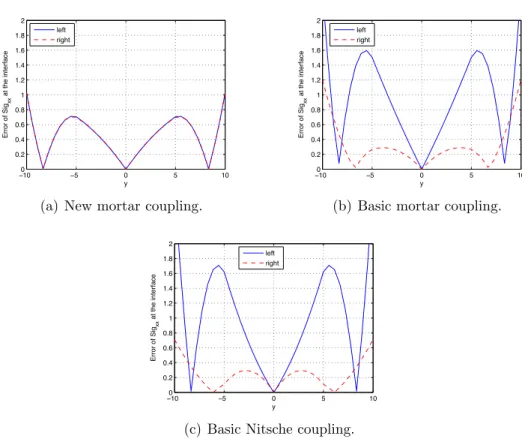
9 10 11 12 13 14 15 16 17 18 19 20 21 22 23 24 25 26 27 28 29 30 31 32 33 34 35 36 37 38 39 40 41 42 43 44 45 46 47 48 49 50 51 52 53 54 55 56 57 −100 −5 0 5 10 0.2 0.4 0.6 0.8 1 1.2 1.4 1.6 1.8 2 Error of Sig xx at the interface y left right
(a) New mortar coupling.
−100 −5 0 5 10 0.2 0.4 0.6 0.8 1 1.2 1.4 1.6 1.8 2 Error of Sig xx at the interface y left right
(b) Basic mortar coupling.
−100 −5 0 5 10 0.2 0.4 0.6 0.8 1 1.2 1.4 1.6 1.8 2 Error of Sig xx at the interface y left right
(c) Basic Nitsche coupling.
Figure 9: Evolution of the exact error of σxxalong the coupling interface for the modeling
9 10 11 12 13 14 15 16 17 18 19 20 21 22 23 24 25 26 27 28 29 30 31 32 33 34 35 36 37 38 39 40 41 42 43 44 45 46 47 48 49 50 51 52 53 54 55 56 57
rect representation of the behavior at the interface (note that the error scale is multiplied by a factor of ten in contrast to the other solutions). Such a be-havior was expected here since the whole derivative fields (i.e., all the strain and stress components) are C0 at the interface for a C1 solution, which is
meaningless from a physical point of view. On the contrary, putting a C0line
at the interface enables to significantly reduce the error (see Fig. 8(e)). As before, we observe that the classical coupling approaches (Figs. 8(b) and 8(c)) are able to represent a C0 solution at the interface. Now, what is interesting
to observe here is that our proposed coupling approach seems to be efficient as well to address bi-material interfaces (see Fig. 8(a)). This is due to the fact that the quantities that are transmitted from one model to the other (the discrete displacement and the traction coming from the discrete dis-placement) are consistent with the initial mechanical problem. In the new coupling solution (Fig. (8(a))), only these quantities are continuous but not the whole derivatives as in the reference C1 solution. We therefore end up
with a coupled solution that is meaningful at a physical point of view, and that enables a better transition of the information at the coupling interface, which leads to a global diminution of the coupling error (see Fig. (9)). 5.1.4. Coupling of non-matching meshes.
The coupling of non-matching NURBS meshes is now investigated. For that, the problem of Fig. 4 is computed again with E11 = E2 = 1000 for
a two non-matching meshes model composed of 5× 3 elements in Ω11 and
5× 5 elements in Ω2. The distribution of the exact error of σxx around the
coupling interface is shown in Fig. 10. The evolution of the exact error at each side of the interface with respect to the vertical coordinate y is also
9 10 11 12 13 14 15 16 17 18 19 20 21 22 23 24 25 26 27 28 29 30 31 32 33 34 35 36 37 38 39 40 41 42 43 44 45 46 47 48 49 50 51 52 53 54 55 56 57
plotted in Fig. 11 before showing the stress jump across Γ in Fig. 12.
Interface
(a) New mortar coupling.
Interface
(b) Basic mortar coupling.
Interface
(c) Basic Nitsche coupling.
Figure 10: Distribution around the coupling interface of the exact error of the stress
component σxx for a two non-matching meshes model (5× 3 knot-span elements in Ω11
and 5× 5 in Ω2).
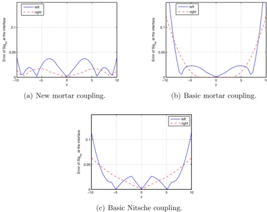
Some error concentrations can be observed at the coupling interface for every method due to the use of non-matching meshes. Once again, it appears that the proposed method results in lower error concentrations (particularly at the exterior boundaries) due to lower stress jumps at the coupling interface. 5.1.5. Convergence behavior in strain energy.
As it has been done for classical mortar and Nitsche couplings (see, e.g., [9, 26, 23]), we finally check the convergence of the new mortar coupled solution with respect to the refinement of the mesh. In order to do so, we consider again the problem of Fig. 4 (with E11 = E2 = 1000) and we proceed as
9 10 11 12 13 14 15 16 17 18 19 20 21 22 23 24 25 26 27 28 29 30 31 32 33 34 35 36 37 38 39 40 41 42 43 44 45 46 47 48 49 50 51 52 53 54 55 56 57 −100 −5 0 5 10 0.05 0.1 Error of Sig xx at the interface y left right
(a) New mortar coupling.
−100 −5 0 5 10 0.05 0.1 Error of Sig xx at the interface y left right
(b) Basic mortar coupling.
−100 −5 0 5 10 0.05 0.1 Error of Sig xx at the interface y left right
(c) Basic Nitsche coupling.
Figure 11: Evolution of the exact error of σxx along the coupling interface for the two
non-matching meshes model.
−10 −5 0 5 10 −0.4 −0.3 −0.2 −0.1 0 0.1 0.2 0.3 0.4 Jump of sig xx at the interface y New mortar coupling Basic mortar coupling Basic Nitsche coupling
Figure 12: Jump of σxx along the coupling interface for the two non-matching meshes
9 10 11 12 13 14 15 16 17 18 19 20 21 22 23 24 25 26 27 28 29 30 31 32 33 34 35 36 37 38 39 40 41 42 43 44 45 46 47 48 49 50 51 52 53 54 55 56 57
energy error is computed as:
|Eex− Ef e|
Eex
, (29)
where Ef e denotes the strain energy of the NURBS finite element model and
Eexdenotes the reference exact strain energy equals to 3296 according to [46].
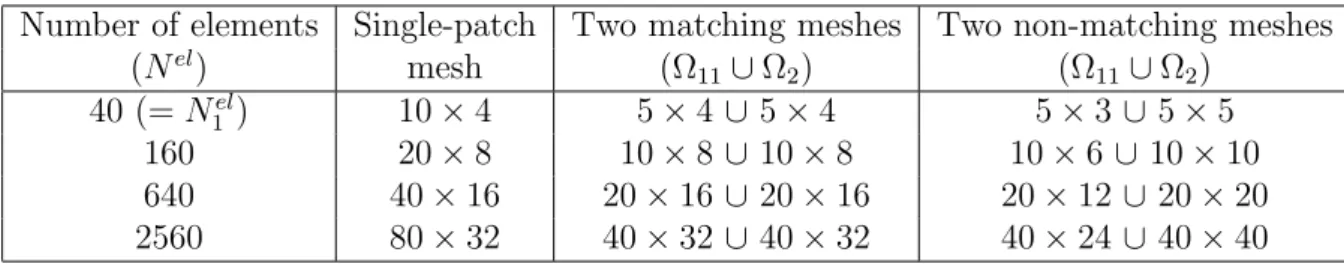
The coupling of matching and non-matching meshes is investigated. For the refinement, the meshes indicated in Tab. 1 are used. We recall that quadratic NURBS meshes are considered, the continuity at the interior lines (and so, at the interface) being C1. The convergence curves are finally plotted in
Fig. 13 with respect to the equivalent number of elements Nel normalized by
the number of elements Nel
1 of the equivalent single-patch coarsest mesh (see
left column of Tab. 1 for the associated values).
Number of elements Single-patch Two matching meshes Two non-matching meshes
(Nel) mesh (Ω 11∪ Ω2) (Ω11∪ Ω2) 40 (= Nel 1 ) 10× 4 5× 4 ∪ 5 × 4 5× 3 ∪ 5 × 5 160 20× 8 10× 8 ∪ 10 × 8 10× 6 ∪ 10 × 10 640 40× 16 20× 16 ∪ 20 × 16 20× 12 ∪ 20 × 20 2560 80× 32 40× 32 ∪ 40 × 32 40× 24 ∪ 40 × 40
Table 1: Meshes considered to study the convergence behavior.
We observe that the convergence rate and the error constant of the cou-pled discretizations are equivalent to the ones of the equivalent single-patch discretization. As emphasized above, the solutions are exactly the same for matching meshes (see Fig. 13(a)). For sure, a slight discrepancy appears for non-matching meshes (see Fig. 13(b)) since in this case the single-patch model cannot exactly represent the coupled model. These convergence curves demonstrate that the developed coupling method does not interfere with the
9 10 11 12 13 14 15 16 17 18 19 20 21 22 23 24 25 26 27 28 29 30 31 32 33 34 35 36 37 38 39 40 41 42 43 44 45 46 47 48 49 50 51 52 53 54 55 56 57 100 101 102 10−8 10−7 10−6 10−5 10−4 |Eex − Efe |/Eex N /N p=2, 1 domain p=2, 2 subdomains 1 el el
(a) Matching meshes.
100 101 102 10−8 10−7 10−6 10−5 10−4 |Eex − Efe |/Eex N /N1 p=2, 1 domain p=2, 2 subdomains el el (b) Non-matching meshes.
Figure 13: Convergence of the strain energy for uniform refinement in both subdomains.
global increased accuracy achieved by the NURBS functions.
5.2. Plate composed of a trimmed B-spline patch and a circular NURBS domain
With the next example, the coupling of non-conforming geometries is investigated (see Fig. 2(c) as a reminder). The test case concerns an ho-mogeneous rectangular plate subjected to constant in-plane tension (see Fig. 14(a)). The geometric model of the plate consists of a quadratic trimmed B-spline patch and a quadratic circular NURBS domain that are connected via a circular NURBS curve (see Fig. 14(b) for illustration). Since the con-necting curve is inside the quadratic B-spline patch, the continuity of the basis functions of Ω11 along Γ is at least C1. To build the NURBS circular
domain Ω2, we extract it from a larger quadratic NURBS patch containing
an additional layer of two elements (following the strategy depicted in re-mark 3). In this way, the continuity of the basis functions of Ω2 is C1 at the
interface Γ. We finally make use of a fictitious domain method to compute the solution on the grey part of the two NURBS entities.
9 10 11 12 13 14 15 16 17 18 19 20 21 22 23 24 25 26 27 28 29 30 31 32 33 34 35 36 37 38 39 40 41 42 43 44 45 46 47 48 49 50 51 52 53 54 55 56 57 Sym L H p R
(a) Description and data of the problem.
coupling
Trimmed B-spline patch
NURBS domain
(b) Discretization of the coupling problem.
Figure 14: Plate under uniaxial stress modeled by a trimmed B-spline patch and a circular NURBS domain.
9 10 11 12 13 14 15 16 17 18 19 20 21 22 23 24 25 26 27 28 29 30 31 32 33 34 35 36 37 38 39 40 41 42 43 44 45 46 47 48 49 50 51 52 53 54 55 56 57
The results in terms of displacement and stress of the two-domain problem using the new mortar and classical mortar couplings are given in Fig. 15. The correct displacement seems to be obtained with the two coupling strategies. However, a discontinuity of the stresses can be observed with the classical mortar coupling which leads to some error concentrations at Γ (see Fig. 15(d), the desired stress being p = 10). The discontinuity seems to completely disappear in the new mortar coupling solution, which goes with a diminution of the maximum level of error.
5.3. Non-intrusive analysis of a frame
In the third example, the non-intrusive algorithm (25)-(26) is investigated for the coupling of two non-matching meshes model. A plane frame analysis is performed to this end. The numerical problem considered is taken from Nguyen et al. [24] where a reference solution is provided. As an application of the use of the non-intrusive coupling strategy, we propose to illustrate, with this problem, the possibility of making non-intrusive NURBS local re-finement.
The numerical model is described in Fig. 16. Due to symmetry, only half of the problem is analysed with appropriate symmetric boundary conditions. For the discretization of the problem, a C0 line is set up between the two
arms since the geometry at this location is C0. To get a good accuracy, a
quadratic NURBS patch composed of 2 elements into the thickness direction has been considered for the global model. Into the length direction, we take 8 elements for the vertical arm and 4 elements for the horizontal one. The local model, located into the corner, is composed of a quadratic mesh of 8 (thickness direction) ×4 (length direction) for both the vertical and the
9 10 11 12 13 14 15 16 17 18 19 20 21 22 23 24 25 26 27 28 29 30 31 32 33 34 35 36 37 38 39 40 41 42 43 44 45 46 47 48 49 50 51 52 53 54 55 56 57
(a) New mortar coupling: disp. uy.
(b) New mortar coupling:
VM stress σvm.
(c) Basic mortar coupling: disp. uy.
(d) Basic mortar coupling:
VM stress σvm.
Figure 15: Coupled solution for the plate composed of a trimmed B-spline patch and a circular NURBS domain (top: new mortar coupling, bottom: basic mortar coupling).