Advanced controls and measurements for the injection molding of a short fiber reinforced polymer

(1)

HAL Id: hal-01796850

https://hal.archives-ouvertes.fr/hal-01796850

Submitted on 5 Mar 2019

HAL is a multi-disciplinary open access archive for the deposit and dissemination of sci-entific research documents, whether they are pub-lished or not. The documents may come from teaching and research institutions in France or abroad, or from public or private research centers.

L’archive ouverte pluridisciplinaire HAL, est destinée au dépôt et à la diffusion de documents scientifiques de niveau recherche, publiés ou non, émanant des établissements d’enseignement et de recherche français ou étrangers, des laboratoires publics ou privés.

Advanced controls and measurements for the injection

molding of a short fiber reinforced polymer

Gilles Saint Martin, Christophe Levaillant, P. Devos, Fabrice Schmidt

To cite this version:

Gilles Saint Martin, Christophe Levaillant, P. Devos, Fabrice Schmidt. Advanced controls and mea-surements for the injection molding of a short fiber reinforced polymer. PPS-18 -18th annual meeting of polymer processing society, Jun 2002, Guimaraes, Portugal. 17p. �hal-01796850�

(2)

Advanced Controls and Measurements for the

Injection Molding of a Short Fiber Reinforced Polymer

G. Saint-Martin(a,*)_{, F. Schmidt}(b)_{, P. Devos}(c)_{, C. Levaillant}(b)

(a)_{Technofan, 10 Place Marcel Dassault, B.P. 53 - ZAC Grand Noble, 31702 Blagnac Cedex, France} (b)_{Ecole des Mines d'Albi-Carmaux, Campus Jarlard, route de Teillet, 81013 Albi Cedex 9, France}

(c)_{DRIRE Midi Pyrénées, 12 rue Michel Labrousse, B.P. 1345, 31107 Toulouse Cedex 1, France} (*)_{Corresponding author}

Abstract

This study is a collaboration between Technofan, Microturbo, Liebherr Aerospace, CROMeP and LGMT. It is a four years project focused on the optimization of the injection molding process, applied to short fiber reinforced polymers, in order to work on :

- The mechanical properties improvement of the molded parts ; - The reduction and the reinforcement of parts structural defects ; - The prediction of mechanical properties.

The aeronautic sector generalizes its policy of aluminum's substitution by reinforced polymers. The main advantages of these materials are a low cost and a low mass. Our study focuses on the Ultem 2300-1000 polyetherimide resin from General Electric Plastics. The injection molding process allows to realize very complex shapes in one step, but can also generates some important defects. The main defects studied in this paper are weldlines and voids.

First, we present a detailed characterization of these defects which includes weldlines, meldlines and voids in thick zones. Then, we present the results of some experiment series realized in order to clarify the dependence between the defects and the injection molding process. A reinforcement of the meldlines has been obtained by modifying the symmetry of the mold cavity. This effect is simulated with Moldflow software, and a quantitative comparison is achieved between experimental and numerical fiber orientation. Then, we apply different non-destructive control methods (like ultrasonic controls or density measurements) in order to retain the most relevant ones for the detection of voids and for their application in the aeronautic industry. Finally, we present an original process control method that can help to detect if there is a risk of void for thick parts at the very first stage of the injection molding production process.

1- Introduction

A policy of weight reduction of airplanes has been followed for the last ten years. Equipment designers have been trying to substitute conventional metallic alloys (steel, titanium, aluminum) by injection molded high properties polymers, for semi-structural airplanes parts. Consequently, there is currently a considerable interest in short fiber reinforced thermoplastic composites. These materials are easily processed and they also offer advantages of low cost and mass or special characteristics (chemical and fire resistance), very useful in the aeronautic field. The injection molding process allows to create very complex shapes without post machining and can even be justified with relatively short series (typically lower than 1000 units per year). Unfortunately, studies over many years (1, 2, 3) have shown quite complicated fiber orientations which depend on a lot of parameters and on the cavity geometry. Even if there are good previsions of fibers orientation in simple shapes, almost all-industrial cases are more complicated because of product shapes and mechanical requirements. This is a problem for the part designing phase which need accurate information about mechanical characteristics and fibers orientations. The injection molding process also generates very critical defects such as weldlines, meldlines and voids.

Firstly, we briefly present our injection molding machine layout and the molds we use. These different mold cavities have been designed to study the defects and to realize transpositions to industrial applications.

(3)

Meldlines are created when at least two flow fronts join themselves with parallel trajectories (4). It is a common phenomenon which appears during the mold filling stage. The aeronautic industry uses very complex parts (fan wheels, butterfly valves, etc.) which often include a lot of meldlines. This is an important problem acting on the mechanical behavior of the products. Our work consists in a characterization of meldlines morphologies. We study the influence of a deviation volume during the filling stage and on mechanical properties of center-gated ISO tensile test specimens. Then we use Moldflow software in order to simulate the injection molding cycles. The numerical fiber orientation results will feed a mechanical program calculating the specimen properties. Finally, mechanical and orientation data from experiments and calculations can be compared.

According to literature and to our experiments, voids seem to be initiated during the filling stage. But they are mainly influenced by the packing, holding and cooling stages (5). The substitution of the metal parts with injection molded polymeric parts leads frequently to fill important thickness. This is highly generator of void risk. Therefore, the mechanical behavior can be degraded. As this problem has not been studied a lot, we first realize morphological characterizations of the voids in thick parts. Different non-destructive testing (NDT) methods have been evaluated for this application. Then we use sensors data for the entire injection molding cycle. A void creation empirical model (VCEM) is then

proposed and results are compared to NDT and morphological experimental results.

2- Injection Molding Experiments

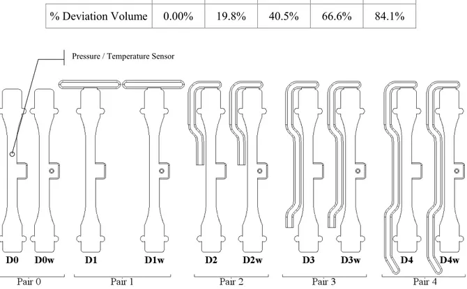
The injection molding machine is a DK Codim 5.02/175/600, 175 tons of clamping force, with an oil mold temperature regulation system (up to 230°C), and electric barrel heaters (up to 430°C). A data acquisition system gets signals from the machine (hydraulic pressure, reciprocating-screw parameters, etc.) and from in-mold transducers (temperature and pressure). A modular mold is used in order to realize different part shapes with a minimum cost. Figure 1 shows the injection molding machine and details of the modular mold.

The main mold cavities used for our work are represented in figure 2. All parts are molded by pairs with one instrumented and one for post-molding characterizations.

Figure 1 - Injection Molding Machine and Modular Mold

Figure 2 - Experimental Mold Series

(4)

Pair A corresponds to ISO tensile test specimen that can be molded with or without weldline. Pair B corresponds to ISO tensile test specimen that can be molded with different deviation configuration of the meldline. Pair C is a 7mm thick plate that can be molded with or without meldline. Pair D is a derived geometry from an industrial part (fan wheel presented in figure 22) that corresponds to a thick divergent plate including a thin perpendicular pale.

The material used in this study is a 30% short fiber reinforced polyetherimide from General Electric Plastics, commercialized with the label "Ultem 2300-1000". Other grades with different reinforcement levels (from 0% to 40%) are also used for special experiments focused on fibers effect. Different parameters are studied. The first step consists in processing Taguchi experiment series. They lead to define the parameters that influence the results in terms of defects, mechanical characteristics, fibers orientations, etc. Then, we realize other more classical experiments with refined parameters variation steps.

3- Meldlines Study

The generic term "weldline" includes two types of defects. Weldlines correspond to the junction of two opposite flow fronts. Meldlines correspond to the junction of two non-opposite (frequently almost parallel) flow fronts. Considering the mechanical behavior, weldlines have the worst effect, especially for reinforced polymers. Moreover, it is very difficult to get a significant improvement of the weldline mechanical resistance by acting on process parameters. This point has been largely studied in the literature (4). Meldlines are very interesting because of two aspects. Firstly, considering complex industrial parts, a lot of meldlines are formed during the filling stage (4). Secondly, a modification of the defect formation phase can highly improve the defect morphology, and as well its mechanical behavior.

3.1- Fiber Orientation Measurements

Injection molded ISO specimens (see figure 2-B) are cut in the meldline region. A fine polishing step (1µm roughness disk) until the average plane is processed (see figure 3). The meldline region is then entirely observed with a Scanning Electron Microscope (SEM) at fixed magnification and electron-beam conditions. SEM images are then treated in order to get fibers orientation information represented by the Advani tensor (6). An average orientation tensor is finally calculated for each image which are assembled in the part reference (see figure 3).

z x

y

Injection Gate

Image Analysis Region Meldline

x

y z

Raw SEM Image Post Analysis Image

Figure 3 - Fibers Orientation Experimental Measurements

ϕ θ

(5)

3.2- Mechanical characterizations

A conventional ISO tensile test is used for the mechanical characterization of meldlines. The equipment is an Instron 4467 of with a 30kN load cell. For each process and mold configuration, ten pairs of specimen are tested. Each pair corresponds to a meldline-included part, and to a no-meldline part (reference). This allows the calculation of meldline factors for each specimen pair. Process parameters we study are : hydraulic holding pressure, mold temperature and polymer temperature (nose temperature). The mold configurations that influence the meldline deviation are presented in table 1 and figure 4. All specimen gates are cuted before testing in order to have similar section.

Table 1 - Deviation Volume Configurations

D0 D1 D2 D3 D4

% Deviation Volume 0.00% 19.8% 40.5% 66.6% 84.1%

Table 2 shows holding pressure and mold / polymer temperature levels used for our experiments. Table 2 - Experimental Process Parameters Levels

Holding Pressure [MPa] 5 7.5 10 12.5 15

Mold Temperature [°C] 140 160 180

Polymer Temperature [°C] 380 400 420

Considering temperatures (see figure 5), increasing the gap between polymer and mold temperature results in a better specimen rigidity (Young modulus) and in a better tensile strength. The deviation effect also appears in figure 5 between D0w and D3w configurations.

Pressure / Temperature Sensor

(6)

The hydraulic holding pressure level has no significant influence on the mechanical properties of the meldline, but has an important effect on the reference specimen (no meldline). On a contrary, the deviation volume configuration has no significant influence on the reference specimen, and a strong effect on the meldline mechanical behavior. These results are represented in figure 6.

Therefore, an important deviation volume rate can lead to the meldline loss (meldline factor reaches 0.98). This result can appear for high holding pressure levels.

3.3- Injection Molding Simulation

We use Moldflow_{MPI 2.0 software package for the simulation of the injection molding process. As}

shown in figure 7, both specimens parts, runners and sprue are simulated. This choice had been done in order to represent as close as possible the experimental conditions for further comparisons.

The mesh is realized using Moldflow modeler and is refined in the meldline region. The rheological parameters of the Ultem 2300-1000 (GE4106 in Moldflow database) are set to default values. For our comparisons, we adjust the cycle conditions in order to fit experimental pressure data at points A and B (pressure sensors locations).

The calculated fibers orientation results can be extracted as one Advani tensor for each mesh element. A Krigging interpolation method (7) is then applied to both experimental and simulated results in the

Tensile Strength [MPa] Polymer Temprature [°C] Mold Temperature [°C] D3 D0w Maximum

Figure 5 - Effect of Mold and Polymer Temperature on the Mechanical Properties of the Meldline

Mold Temperature [°C] Polymer Temperature [°C]

D3w

Figure 6 - Effect of Holding Pressure and Deviation Volume on the Meldline Mechanical Behavior

Tensile Strength [MPa]

Deviation Volume [%] Holding Pressure [x10 MPa]

Meldline Factor

Deviation volume [%]

Experimental Points

(7)

meldline region. Consequently, we have the capability to quantify the gap existing between experimental and simulated fibers orientations (8).

In a regular case (no meldline), experimental and simulated fibers orientations are in very good agreement. The choice of the meldline region had been done in order to test the limitations of Moldflow_{. Figure 9 show the results for D0, D2 and D4 deviation volume configurations. The a}

11

value corresponds to the first Advani tensor term in the part reference (see figures 3 and 8) which is defined below :

ú

û

ù

ê

ë

é

=

θ

ϕ

θ

ϕ

θ

ϕ

θ

ϕ

θ

ϕ

θ

ϕ

θ

ϕ

θ

ϕ

θ

²

cos

sin

cos

sin

cos

sin

cos

sin

²

sin

²

sin

cos

²

sin

cos

sin

cos

²

sin

²

cos

²

sin

a

(1) D0

Figure 7 - The D0 Numerical Model for Injection Molding Simulations

Meldline Specimen Reference Specimen B A x y z θ

(a)

x y a b B A φ

(b)

Figure 8 - Definition of Fiber Orientation Angles

÷ ø ö ç è æ = A B Arc tan

φ

(2) ÷ ø ö ç è æ = a b Arc cos

θ

(3)

(8)

All configurations present a good qualitative agreement between experimental measurements and calculation results. The average absolute difference is lower than 0.2 on the a11 value for the majority

of the surface. The critical zone is located at the very beginning of the meldline (close to the pawn). The deviation effect that leads to make the a11 surface higher on the experimental measurements is

also reported by the calculations.

4- Voids Study

Voids can appear in injection molded parts when the thickness becomes important. Typically, a thickness greater than 5mm is difficult to mold without void. Geometric particularities like ribs or section changes can also generate some voids. Considering the mechanical resistance of the molded part, this kind of defect is very important. A void leads to a stress concentration and can create some cracks. Voids generation has not been intensively studied in the literature. Anyway, some interesting articles had been published for the last ten years (5, 9, 10, 11). Industrial parts including voids can seriously be damaged during their utilization. When a part region has an important thickness, it is often due to high stresses applied on. Then, if voids exist in this region, a braking can quickly appears. Therefore, the methodology we have is to optimize the process and the part design in order to avoid this type of defect that is not acceptable.

Figure 9 - Experimental and Simulated Fiber Orientation Results for the Meldline Region

a11 a11 a11 a11 a11 a11 D0 D0 D2 D2 D4 D4 Measurement Simulation Measurement Simulation Measurement Simulation x [µm] x [µm] x [µm] x [µm] x [µm] x [µm] y [µm] y [µm] y [µm] y [µm] y [µm] y [µm]

(9)

4.1- Non-Destructive Testing and Voids Evaluation

Injection molded thick plates levels (see figure 2-C) are produced using different hydraulic holding pressure. All the other process parameters are kept constant. Figure 10 shows the polymer pressure evolution for different holding levels (holding time remains constant). The pressure sensor is located in the center of the plate.

For voids detection, we have evaluated different non-destructive testing methods (x-ray computer-tomography, infrared detection, ultrasonic detection, etc.). In our case, the best result in terms of cost and availability has been given by density measurement method (norm ISO 1183). Interesting results has also been given by ultrasonic NDT method (12) which is very sensitive to density variation. Density measurements give a derived global information about the void content of the part. The ultrasonic C-scan method can provide 2D density cartography across the part (13). It is also possible to realize B-scan tests in order to get 3D information.

Figure 11 - Ultrasonic C-scan of a Thick Plates Molded with Different Holding Pressure Levels

Holding Pressure = 0 MPa Holding Pressure = 1 MPa Holding Pressure = 2.5 MPa

Holding Pressure = 5 MPa Holding Pressure = 7.5 MPa Holding Pressure = 10 MPa + -U ltr as on ic S ign al A m pl itu de

Figure 10 - Polymer Pressure Evolution in the Mold Cavity for Different Holding Levels

12 MPa 10 MPa 7.5 MPa 5 MPa 2.5 MPa 1 MPa 0 MPa Po ly me r Pre ss ure [M Pa ]

Hydraulic Holding Pressure Increases (Holding Time Remains Constant)

(10)

Figure 11 shows the ultrasonic cartography of the thick plate molded with different holding levels. Inspections are processed using a Krautkramer US1P-12 ultrasonic unit linked to a focalized sensor, an Andscan (Defense Research Agency) software, and to an independent electric command. All scans are realized in amplitude variation mode. High density gives high signal amplitude, and as well low density gives low signal amplitude (linear relationship). According to this method, the void content appears to equals zero for hydraulic holding pressure greater than 75 bar. Then, the more the pressure level is low, the more the void content is high. Then we can define an apparent ultrasonic void content parameter VCUS from the cartography by quantifying the white surface (the lowest apparent density).

A traditional cutting and observation method has also been processed in order to compare it with the NDT results (ultrasonic control and density measurement). Each plate is cuted along the width (10 samples per plate). Samples are polished and observed using an optical microscope. Voids are then isolated and their total surface is quantified. A pseudo-volume optical void content VCO can then be

defined. Figure 12 shows the voids morphology in the plate section for different holding pressure levels. Voids are larger on both sides and are also located in intermediate thickness regions.

The void content parameters VCUS and VCO have an almost linear dependence with the holding

pressure level under 7.5 MPa (see figure 13). The apparent density _ρapp presents a saturation effect for

high holding pressure levels.

Figure 12 - Voids Morphology and Location in Thick Injection Molded Plates

0 MPa 5 MPa 10 MPa 20mm 2mm 2mm 1,43 1,44 1,45 1,46 1,47 1,48 1,49 1,50 1,51 1,52 1,53 0 1 2 3 4 5 6 7 8 9 10 0 1 2 3 4 5 6 7 0 1 2 3 4 5 6 7 8 9 10 VCUS VCO

Figure 13 - Void Content and Apparent Density Versus Holding Pressure

Holding Pressure [MPa] Holding Pressure [MPa]

Appar

ent Dens

(11)

4.2- Void Creation Empirical Model (VC

EM

)

Our goal is to define an empirical void creation model which can be used as a quality control tool for industrial productions. According to literature and to our knowledge (5, 8, 9, 10, 11), all injection molding stages have to be taken into account : filling, packing, holding and cooling.

The thermal regime is defined by the evaluation of the Cameron number :

2

h V

aL

Ca= (4)

If Ca is lower than 0.01, the regime is adiabatic. If Ca is greater than 1, there is an equilibrium regime. Between theses two values, there is a thermal transition regime (14). Our case leads to an adiabatic regime (Ca = 0.0028).

Moldflow is used for the evaluation of the temperature profile along the thickness and across the part. Simulation and process parameters are set and adjusted in order to have a good agreement with the experimental pressure measurements (see figure 15).

As Moldflow does not allow to get all calculation results in numerical format, we use temperature-thickness curves for different positions labeled from 0 to 4 (see figure 15). Temperature profiles do not change significantly along the part's width (y coordinate) except in the diverging entrance, but changes significantly along the part's length (x coordinate) (see figure 16).

u(z) z x y h L X Sensor (∆p, T0)

Figure 14 - Boundary Conditions for the Filling Stage of the Thick Plate

TMold

Comparison and Calculation Points Sensors Locations

Figure 15 - Part Mesh, Comparison and Calculation Points

Calculation Points x y z 4 3 2 1 0 Pressure/Temperature Transducer

(12)

Since temperature profiles along thickness are known at the end of the filling stage for different locations (T_ef(z)_X, X = 0 to 4 as shown in figure 15), the next step consists in working on the packing, holding and cooling stages. Theses phases have in common a negligible polymer movement. We adapt Carlslaw and Jaeger cooling model (15). Sensor temperature data corresponds to the mold temperature

T

_Mold

(t

)

, sensor pressure data corresponds to the polymer pressure (assumed homogeneous), and the time origin is fixed at the end of the filling stage. Then we are able to calculate the polymer temperature

T

(

z

,

t

)

_X at each time step and position along the thickness.

200 250 300 350 400 450 -3,5 -3 -2,5 -2 -1,5 -1 -0,5 0 0,5 1 1,5 2 2,5 3 3,5 X = 0 X = 1 X = 2 X = 3 X = 4 z [mm] Po ly m er Tem per at ur e [° C]

Figure 16 - Simulation Temperature Results at the End of Filling Stage

x

y

(13)

[

]

2 ( ) 2 1 cos 2 1 ) 1 ( ) ( ) ( 2 ) , ( 0 4 2 1 2 2 2 t T h z n n t T z T t z T _Mold n h at n n Mold x ef x

e

+ ÷ ÷ ÷ ÷ ø ö ç ç ç ç è æ ú û ù ê ë é ÷ ø ö ç è æ + ⋅ ⋅ ÷ ø ö ç è æ + − ⋅ − =

å

∞ = ÷ ø ö ç è æ + −

π

π (5)

The polymer temperature evolutions during packing, holding and cooling phases are represented in figure 17 for each calculation location (X = 0 to 4).

Since the polymer cools inside the mold cavity, the pressure decreases, depending on the hydraulic holding level (see figure 10). Considering the polymer no-flow temperature Tnf (General Electric

Plastics data), we can calculate the pressure at the no-flow boundary p*(z). For this calculation, we use the sensor pressure data and we consider that polymer pressure is uniform along thickness. Therefore, we have different p*(z) profiles depending both on the holding level and on the location, as shown in figure 18 in the particular case of location 2.

X = 0 X = 1 X = 2

X = 3 X = 4 The horizontal line corresponds to the solidification boundary.

Cooling phase is represented from t = 0s (end of filling stage) to t = 65s. The thickness is divided into 21 layers.

Figure 17 - Polymer Cooling for Different Locations in the Part

Po ly m er te mp er at ur e [° C ] Po ly m er te mp er at ur e [° C ] Po ly m er te mp er at ur e [° C ] Po ly m er te mp er at ur e [° C ] Po ly m er te mp er at ur e [° C ] z [mm] z [mm] z [mm] z [mm] z [mm]

Figure 18 - Pressure at the No-Flow Boundary along Thickness for Different Holding Levels

LV z [mm] z [mm] z [mm] z [mm] z [mm] z [mm] N o-F lo w P re ss ure [M pa ] N o-F lo w P re ss ure [M pa ] N o-F lo w P re ss ure [M pa ] N o-F lo w P re ss ure [M pa ] N o-F lo w P re ss ure [M pa ] N o-F lo w P re ss ure [M pa ] Holding Pressure 0 MPa Holding Pressure 1 MPa Holding Pressure 2.5 MPa Holding Pressure 5 MPa Holding Pressure 7.5 MPa Holding Pressure 10 MPa

(14)

We assume that the void content rate depends on the volumetric shrinkage applied to the polymer at the no-flow boundary (16). In order to evaluate this assumption, we use a pvT Tait model defined using General Electric Plastics data (see figure 19).

When the pressure reaches zero and the polymer is solidified, shrinkage appears. If we consider the no-flow boundary (defined by the temperature), we assume that there is a void formation (instead of shrinkage) in all area where p*(z) = 0. The volumetric shrinkage (

v

_sol

−

v

₀) is evaluated using the pvT diagram (see figure 17). The void content value VCEM is then defined as :

(

)

ò

−

⋅

=

2 0 0

2

V L nf C EM

v

dz

h

A

VC

(7)

Where LV is the length of the thickness where p*(z) = 0 (see figure 18). AC is a scale factor introduced

to adjust the VCEM value for further comparisons with other void content parameters (VCO and VCUS).

4.3- Comparison between Experimental Measurements and VC

EM

Results

Figure 20 presents a plot of VCEM (average curve for X = 1 to 4), VCO and VCUS versus the apparent

part density _ρapp. All three parameters present similar evolutions and the same minimum apparent

density (1.52) that insure void free injection molded thick plates. This apparent density value corresponds to a holding pressure level of 7.5 MPa. If the holding pressure is increased over this value, the apparent density does not increase a lot (saturation effect presented in figure 13). For holding pressure values under 7.5 MPa, the lower the apparent density is, the higher the void content is.

Therefore, it is possible to predict empirically the void formation in injection molded parts. We use sensor data (temperature and pressure) and Moldflow filling simulation results (temperature) in order to apply the VCEM and it is possible to transpose this calculation to a process control tool that could

constitute a quality control method.

Figure 19 - The Tait pvT Model of the Ultem 2300-1000

0,64 0,65 0,66 0,67 0,68 0,69 0,70 0,71 0,72 0,73 0,74 270 320 370 420 470 520 570 620 670 NB :

Curves going (from top to bottom) from 0 to 2.108_{Pa, by step of 10}7_Pa

(

)

constant

(

0894

,

0 )

transition

(

And,

e

)

,

(

e

)

(

)

(

For

0 )

,

(

e

)

(

)

(

For

With,

)

,

(

)

(

1 ln

1 )

(

)

,

(

5 6 5 7 3 2 1 0 3 2 1 0 0 9 8 4 4

=

−

=

⋅

+

=

ï

î

ï

í

ì

⋅

=

⋅

=

⋅

+

=

Þ

<

ï

î

ï

í

ì

=

⋅

=

⋅

+

=

Þ

>

+

ú

û

ù

ê

ë

é

÷÷ø

ö

ççè

æ

₊

⋅

−

⋅

=

⋅ − ⋅ ⋅ − ⋅ −

C

b

T

p

b

T

b

p

T

v

b

T

B

T

b

T

v

T

p

T

v

b

T

B

T

b

T

v

T

p

T

v

t

B

p

C

T

v

p

T

v

t p b T b t T b s s s t t T b m m m t t s m vnf v0 Tnf Tair (6) Absolute Temperature [K] Sp eci fi c V olu m e [c m3 /g ]

(15)

A general layout of the quality control method we want to create is presented in figure 21.

5- Conclusions

Both meldlines and void defects do not have the same impact on the mechanical properties of an injection molded part. On one hand, meldlines should be considered as perfectible defect. The deviation method consisting in the creation of a flow through the defect during the filling stage has a good efficiency. Moreover, injection molding simulation tools like Moldflow appear to be able to predict the results in terms of fibers orientation. Extended studies can also lead to a prediction of the

Moldflow_Simulation

VCEM

Experimental Data

Mold Sensor Data Injection Molding

Machine

Simulation Adjustment Void Alert Signal

Figure 21 - Quality Control Method Based on the VCEM

Figure 20 - Void Content Parameters Comparison

0 1 2 3 4 5 6 7 1,42 1,44 1,46 1,48 1,50 1,52 1,54 Apparent Density VCUS VCO VCEM

(16)

mechanical properties modifications (17). On the other hand, voids are not acceptable and the creation of a prediction method that could be used at the production stage is on the way. Injection molding simulation brings again a precious help for this problem.

6- Future Work and Applications

Concerning the meldline defects, future studies will be focused on : - Mesh refinement in the meldline region ;

- Simulation of the complete injection molding process (including packing and holding). Fibers orientation data will also be used in order to realize mechanical calculations based on Moldflow simulations (17). Comparisons between experimental and calculated mechanical properties will finally be done. Fair results had been found about the deviation efficiency on the improvement of meldline mechanical properties. This method will be applied to industrial parts (see figure 22) at the mold designing stage. Runner and gates will be optimized in order to have deviated meldlines.

Moldflow software will also be used in order to generalize this model to the entire part. Several NDT methods have to be applied to industrials cases. Density measurements and ultrasonic controls are mainly studied. Applications to industrial injection molded parts are also planned (see figure 22). Concerning the void defect, future studies will mainly be focused on voids location along the thickness. If we consider fibers orientations, shear rate during filling, and voids location after cooling, it appears that voids are generated in regions where fibers are perfectly aligned in the (x ; y) plane. We assume that in high shear rates regions, the polymer flow leads to no z-alignment for the fibers (Advani tensor term a33 ≈ 0), and this means the polymer matrix is the only barrier against voids

formation. On a contrary, for lower shear rate regions, z-alignment does not equals zero, and fibers can create a barrier against void formation. Therefore, inside the region where p*(z) = 0, the most breakable zone corresponds to the highest shear rate region during filling. Figure 23 presents a superposition of shear rate, fibers orientation and voids location for the thick injection molded plate. In addition, Kumuzawa (16) shows that z-linear shrinkage is much higher than x or y one. Consequently, it is the z-linear shrinkage that mainly explains the formation of voids. Complementary experiments will be processed using Ultem grades having different reinforcement rates (from 0% to 40%) in order to confirm this approach.

(17)

Extended applications to other injection molded parts have also to be done in order to validate the VCEM results in different geometric configurations (see figure 2-D).

Acknowledgements

We thank Dr. R. Zheng (Moldflow_{Pty. Ltd.) for his helpful advice on the orientation calculations.}

The work of S. Proust and E. Jourdain (CROMeP) for experimental measurements, and Moldflow simulations is gratefully acknowledged. We also thank S. Devaux (CRITT of Toulouse) for the helpful availability of his ultrasonic equipment, and O. Darnis (Technofan) for his support. Special thank goes to all collaborating companies (Liebherr, Microturbo, LGMT). This study is realized with the financial support of the European Community, the Midi-Pyrénées Regional Council and of the French Agency of Technical Research.

References

1. T.D. Papathanasiou and D.C. Guell, Flow Induced Alignment in Composite Materials, Woodhead Publishing Ltd (1997)

2. L.A. Carlsson and R.B. Pipes, Thermoplastic Composite Materials, Elsevier (1991)

3. M.C. Altan, A Review of Fiber-Reinforced Injection Molding : Flow Kinematics and Particle

Orientation, Journ. Thermoplas. Compos. Mat., 3, pp. 275-313 (1990)

4. S. Fellahi, A. Meddad, B. Fisa and B.D. Favis, Weldlines in Injection-Molded Parts : A Review, Adv. Polym. Tech., 14, pp. 169-195 (1995)

5. M. Akay, D.F. O'Regan, Generation of Voids in Fiber Reinforced Thermoplastic Injection

Moldings, Plas. Rubb. Compos. Proc. Appl., 24, pp. 97-102 (1995)

z x

y

Voids Morphology Calculated Shear Rate Profile

Fiber Orientation

1mm

(18)

6. S.G. Advani, C.L. Tucker, A Tensor Description of Fiber Orientation in Short Fiber Composites, SPE-ANTEC Tech. Papers, pp. 1113-1118 (1985)

7. F. Trochu, A Contouring Program Based on Dual Krigging Interpolation, Engineering with Computers, 9, pp. 160-177 (1993)

8. G. Saint-Martin, F. Schmidt, C. Levaillant, P. Devos, Fiber Orientation of Meldlines in Injection

Molding of Fiber Reinforced Thermoplastic : A Quantitative Comparison of Experimental and Numerical Results, Submitted to Polymer Composites (March 2002)

9. G.L. Beall, Thick Walls Encourage Sink Marks and Voids, Kunststoffe German Plastics, 82, 9, pp. 62-64 (1992)

10. M. Akay, D.F. O'Regan, Generation of Voids in Fiber Reinforced Thermoplastic Injection

Moldings, Plas. Rubb. Compos. Proc. Appl., 24, pp. 97-102 (1995)

11. M.J. Jaworski, Using CAE Injection Molding Simulation to Predict Overpack, Voids and Sink, SPE-ANTEC Tech. Papers, pp. 3642-3646 (1997)

12. D. Hsu, Ultrasonic Non-Destructive Evaluation of Void Content in CFRP, ANTEC Conf. Proc., pp. 1273-1275 (1988)

13. J. Dumont-Fillon, Contrôle Non Destructifs, Techniques de l'Ingénieur : Traité Mesures et Contrôles, R1400, pp. 1-43 (1999)

14. J.F. Agassant, P. Avenas, J.P. Sergent, P. Carreau, Polymer Processing, Hanser (1991) 15. H.S. Carslaw, J.C. Jaeger, Conduction of Heat in Solids, Oxford University Press (1959)

16. H. Kumazawa, Prediction of Anisotropic Shrinkage of an Injection Molded Part, SPE-ANTEC Tech. Papers, pp. 817-821 (1994)

17. E. Haramburu, F. Collombet, B. Ferret, J.S. Vignes, P. Devos, C. Levaillant, F. Schmidt,

Short-Fiber-Reinforced Thermoplastic for Semi-Structural Parts : Process-Properties, 8th_{Euro-Japanese}

Symposium (2002)