HAL Id: inria-00351894
https://hal.inria.fr/inria-00351894
Submitted on 12 Jan 2009
HAL is a multi-disciplinary open access archive for the deposit and dissemination of sci-entific research documents, whether they are pub-lished or not. The documents may come from teaching and research institutions in France or abroad, or from public or private research centers.
L’archive ouverte pluridisciplinaire HAL, est destinée au dépôt et à la diffusion de documents scientifiques de niveau recherche, publiés ou non, émanant des établissements d’enseignement et de recherche français ou étrangers, des laboratoires publics ou privés.
Visual servoing sequencing able to avoid obstacles.
Nicolas Mansard, François Chaumette
To cite this version:
Nicolas Mansard, François Chaumette. Visual servoing sequencing able to avoid obstacles.. IEEE Int. Conf. on Robotics and Automation, ICRA’05, 2005, Barcelona, Spain, France. pp.3154-3159. �inria-00351894�
Visual Servoing Sequencing Able to Avoid Obstacles
Nicolas Mansard, François Chaumette IRISA - ENS Cachan and INRIA Rennes Campus de Beaulieu, 35042 Rennes, France E-Mail : [email protected]
Abstract— Classical visual servoing approaches tend to
constrain all degrees of freedom (DOF) of the robot during the execution of a task. In this article a new approach is proposed. The key idea is to control the robot with a very under-constrained task when it is far from the desired position, and to incrementally constrain the global task by adding further tasks as the robot moves closer to the goal. As long as they are sufficient, the remaining DOF are used to avoid undesirable configurations, such as joint limits. Closer from the goal, when not enough DOF remain available for avoidance, an execution controller selects a task to be temporary removed from the applied tasks. The released DOF can then be used for the joint limits avoidance. A complete solution to implement this general idea is proposed. Experiments that prove the validity of the approach are also provided.
I. INTRODUCTION
Visual servoing provides very efficient solutions to control robot motions from an initial position to a precise goal [10]. It supplies high accuracy for the final pose, and good robustness to noise in image processing, camera calibration and other setting parameters. However, if the initial error is large, such a control may become erratic [2]. Approaches such as 2-1/2-D[12] or path planning [6], [15] provide solutions that enlarge the region where the system converges. But they each constrain all the avail-able robot DOF from the beginning of the servo. This imposes an unique trajectory to the robot. Particularly, if a new problem, such as an obstacle, is encountered during the task execution, the entire trajectory has to be modified to take it into account. In this paper, we propose to sequence uncomplete tasks until the robot reaches its desired position rather than to use a complete one [16], [20], [17]. Very low constraints are used when the robot is far from the goal, in order to enlarge the trajectories available. Constraints are progressively added as the robot draws near to the required position [13]. When enough DOF are available, they can be used to avoid any undesirable situation [14]. Closer from the required position, when not enough DOF remain available for avoidance, additional DOF are obtained by temporary removing a specific constraint when solving the encountered problem.
A vast number of trajectories are usually available to reach the goal. However, by constraining all DOF from the beginning, the classical control schemes choose a particular trajectory, without knowing if it is valid or not. In some particular cases, this can lead to singularity or instability problems. To always obtain an ideal execution, a first solution is to plan the trajectory, for example by using the potential field method [6], [15]. The idea is to choose an optimal trajectory among all the available
ones. This provides a complete solution, which ensures optimality, stability and physical feasibility to the goal when it is reachable. Path planning solves the deficien-cies of basic approaches, but by applying even stronger constraints to the trajectory of the robot. This means, however, that this solution is less reactive to changes of the goal, of the environment or of the constraints. Rather than deciding in advance which path should be used to reach the goal, switched systems use a set of subsystems along with a discrete switching control [8], [5]. The robot will then avoid difficult regions by switching from a first control law (a particular trajectory) to another one when necessary. This enlarges the stable area to the union of the stable area of each task used. In [13], we described a solution to stack elementary tasks one on top of the others until all degrees of freedom of the robot are constrained, and the desired position is reached. When the robot is far from its desired position, only few DOF are constrained, and the remaining can be used to vary the trajectory, in order to avoid any problem encountered during the execution. Therefore this method does not give satisfactory results when the DOF needed to avoid the problem are already constrained. This is really problematic in the neighborhood of the desired position, when almost all elementary tasks are already stacked.
The key idea of this work is to separate a complete servoing task into several elementary tasks, that are added to a stack when the robot comes closer from the goal. At each step, the robot moves to achieve an elementary task, maintaining all the elementary tasks already completed. At the end, the robot is entirely constrained by the sum of the constraints of each elementary task. Additional constraints such as joint limit avoidance can also be added using the remaining DOF. When these additional constraints can not be ensured because of the lack of appropriate DOF, an elementary task already completed can temporary be released.
In this paper, the structure of the stack of tasks used to sequence the elementary tasks is first defined. A control law is computed that maintains the tasks already achieved when moving the robot according to the last elemen-tary task. This is done by a stack of tasks, using the redundancy formalism introduced in [18]. Contrary to the solution proposed in [13], we rather use the least square resolution method to extend the redundancy formalism to several tasks [19]. The stack also guarantees the continuity of the control law, whatever the manipulation on the stack. We then describe a first general solution to use the remaining DOF for additional constraints such as joint limits avoidance. This method is based on
Proceedings of the 2005 IEEE
International Conference on Robotics and Automation Barcelona, Spain, April 2005
the Gradient Projection Method [14], [11]. This method gives satisfactory results when the robot is highly under constrained (i.e. far from the goal). However the robot behavior is inadequate when the appropriate DOF are already constrained, especially when the robot is almost fully constrained. A method to provide additional DOF when necessary is then proposed. When the additional constraints can not be respected using the Gradient Projection Method, the elementary task that bothers the execution is detected. It is then temporary removed from the stack. When the problem is solved, the removed task can be put back into the stack. Section II presents the structure of the stack. In Section III, the Gradient Projection Method is recalled and applied on the control law obtained in the previous section. A general method to free additional DOF when needed is exposed in Section IV. The experimental results are finally set out in Section V.
II. VISUAL SERVOING USING A STACK OF TASKS
In this section, we expose how to sequence elementary tasks and to maintain the tasks already achieved. The control law is computed from the tasks in the stack, in accordance with two rules:
- any new task added in the stack should not disturb the tasks already in the stack. Particularly, the tasks already completed should remain to zero.
- the control law computed should be continuous, even when a task is added or removed from the stack. The robot is controlled by the articular ve-locity ˙q. A break of continuity means an infinite acceleration during a short period of time, which implies that the control will not be correctly applied. Section II-A presents the redundancy formalism [18]. It has first been used for visual servoing in [7], and in numerous applications since (e.g. avoiding visual occultations [14], or human-machine cooperation using vision control [9]). The idea is to use the DOF left by a first task having priority, to realize a secondary task at best without disturbing the first one. Section II-B sets out the way the redundancy formalism is used to stack several elementary tasks. In Section II-C, we briefly recall the method proposed in [13] to ensure the control law continuity, using a non homogeneous first order differential equation.
A. Redundancy formalism for two tasks
Let q be the articular vector of the robot. Let e1 and
e2 be two tasks, Ji = ∂e∂qi (i = 1, 2) their jacobian,
defined by:
˙
ei=
∂ei
∂qq˙ = Ji˙q (1)
Since the robot is controlled using its articular velocity ˙q, (1) has to be inversed. The general solution (with i = 1) is:
˙
q= J+1e˙1+ P1z (2)
where P1 is the orthogonal projection operator on the
null space of J1 and J+1 is the pseudoinverse (or
least-squares inverse) of J1. z can be used to apply a
sec-ondary command, that will not disturb the task e1having
priority. Here, z will be used to carry out at best the task
e2. Introducing (2) in (1) (with i = 2):
˙
e2= J2J+1e˙1+ J2P1z (3)
By inversing this last equation, and introducing the computed z in (2), we finally get:
˙
q= J+1e˙1+ P1(J2P1)+( ˙e2− J2J+1e˙1) (4)
Since P1is Hermitian and idempotent (it is a projection
operator), (4) can be written: ˙
q= J+1e˙1+ fJ2 +
f˙e2 (5)
where fJ2 = J2P1 is the limited jacobian of the task
e2, giving the available range for the secondary task to
be performed without affecting the first task, and f˙e2 =
˙
e2− J2J+1e˙1is the secondary task function, without the
part J2J+1e˙1of the job already accomplished by the first
task. A very good intuitive explanation of this equation is given in [1].
B. Extending redundancy formalism for several tasks
Let (e1, J1) ... (en, Jn) be n tasks. We want to extend
(5) to these n tasks. Task eishould not disturb task ej if
i > j. A recursive extension of (5) is proposed in [19]:
˙
qi= ˙qi−1+ (JiPAi−1)+( ˙ei− Jiq˙i−1) (6)
where PA
i is the projector onto the null-space of the
augmented Jacobian JA
i = (J1, . . . Ji). The recursion is
initialized by ˙q0= 0. The robot velocity is ˙q= ˙qn.
Using directly this recursive equation, a projector has to be computed on each step of the computation. A recursive formula for the computation of the projector is proposed in [1]. We recall this equation here
PAi = PAi−1− eJi +
e
Ji (7)
where eJi= JiPAi−1 is the limited jacobian of the task i.
The recursion is initialized by PA
0 = I (identity matrix).
C. Smooth transition
Usually, the control law is obtained from the following equation that constrains the behavior of the task function:
˙e= f1(e) = −λe (8)
Since ˙e = J ˙q, we obtain: ˙
q= −λ cJ+e (9)
where cJ+is an approximation of the pseudo-inverse of J
and λ is used as a parameter to control the robot speed.
The f1 function in (8) is chosen by the programmer to
link ˙e and e. One chooses generally f1(e) = −λe to set
an exponential decoupled decreasing of the error. The problem of continuity when changing the task e is due to the lack of constraints on the initial value of
˙e. Let eA be a global task, used to drive the robot until
time t = 0. At this time, the control law switches to a
second task eB. Since e and ˙q are linearly linked, no
continuity guarantee can be ensured on ˙q, at time t=0. In [13], we have proposed to use a non homogeneous first order differential equation to ensure the continuity
and to properly decouple the tuning parameters. The differential equation is
˙e= f2(e) = −λe + ρ(t) (10)
where the non homogeneous part ρ(t) is
ρ(t) = e−µ·t·¡e˙A(0) + λeB(0)¢ (11)
D. Computing the control law
Let (e1, . . . , en) a stack of n tasks. The decreasing
speeds of each task are chosen separately by using
˙e= ˙ e1 .. . ˙ en = − λ1 0 ... 0 λn e1 .. . en = −Λe (12)
Equation (4) can be written ˙q = Lp˙e, where the explicit
expression of Lp is left to the reader. Using (10) and
(12), we deduce the complete expression of the control law computed from a stack of task
½ ˙ qi= ˙qi−1+ (JiPAi−1)+(−λiei− Jiq˙i−1) ˙ q= ˙qn+ e−µ·(t−τ )· ¡ ˙e(τ ) + Λe(τ )¢ (13)
where τ is the time of the last modification of the stack.
III. SIMPLE AVOIDANCE USING THEGRADIENT
PROJECTIONMETHOD
In the previous part, a control law based on a stack of elementary tasks was built, which drives the robot to realize a complete task, such as positioning. This control law is only based on the decreasing of a task function
e (composed of visual features errors in our case). To
integrate the servoing into a complex robotic system, the control law should also make sure that it avoids undesired configurations (such as joint limits, occlusion, obstacles or kinematic singularities). A solution very close from the work presented in Section II is used in [14], based on the task function approach [18]. It is called Gradient Projection Method. A cost function is built that reaches its maximum value at the undesired configurations. This cost function to be minimized is then embedded in a secondary task whose only components that do not affect the primary task are taken into account. This is achieved by projecting the secondary task onto the free space of the primary task.
In the following, we refer to the situations to avoid by the general term obstacles. The experiments presented in Section V have been realized using a joint limits avoidance, but the Gradient Projection Method can be applied to various kinds of obstacles [14], [4]. In this section, we first recall the general method to compute a control law as the gradient of a cost function [7]. The complete control law, using a stack of tasks and additional constraints is then computed. This section will be concluded by the problems encountered using this method, which will introduce the last part of this work.
A. General Gradient Projection Method
In this approach, the robot moves according to a repulsive potential V pushing it away from the obstacles. Let us consider the problem:
min V(q), q∈ Rk (14)
where k is the number of robot articulations. The classi-cal solution is to move the robot according to the gradient of the potential function, computed in the articular space.
˙
q= −κg(q) = −κ∇TqV (15)
where κ is a positive scalar, used as a gain. The secondary task (15) is then projected onto the null space of the primary task, using (2).
B. Gradient Projection Method with a stack of tasks
We want to use the gradient of the cost function as the last task of the stack. The control law (15) has thus to be projected onto the null space of each task into the stack. Using the notations of (13), the complete control law is finally
˙
q= ˙qn+ e−µ·(t−τ)·
¡
˙e(τ ) + Λe(τ )¢− κPAng (16)
Therefore, the avoidance depends on two factors. First
of all, the control law depends on the projector PA
n.
When the stack is almost empty, the rank of PA
n is high,
and the avoidance control law will not be much modified. However when the rank decreases near zero (the stack is almost full), the avoidance control law is highly disturbed, especially if the favorite vector direction of
the gradient is not one of the range of PA
n. Of course,
when the stack is full, the projector becomes 0. The gradient is thus not taken into account any more, and nothing is done to avoid obstacles. The second factor is the gain κ, which defines a priori the influence of the avoidance in the global control law. The choice of this parameter is very important. Indeed, if κ is too small, the gradient force may be too small to avoid the obstacle. Besides, if κ is too high, some overshoot can occur in the computed velocity. Methods that set this parameter automatically exist (for example [4] for the joint limits avoidance). However it is difficult to generalize to an ar-bitrary number of additional constraints simultaneously. Moreover, these methods do not provide any solution to
the problem due to the rank of PA
n.
Instead, the gradient projection method is applied to stay away from the obstacles when it is possible. When this method is not sufficient, the solution is to choose which task of the stack produces the part of the control law that leads the robot in the obstacle, and to remove it from the stack. This solution is detailed in the next section.
IV. USING A STACK CONTROLLER
In this section, a stack controller that removes a task from the stack when necessary is proposed. We also explain how this solution solves the problem presented in the above paragraph.
Two actions are possible on the stack : add a task and remove a task. A task is added when the velocity sent to the robot is under a fixed level, that is to say, when the tasks in the stack are all realized at best, according to their priority range. The order of the tasks to be introduced in the stack are a priori decided. We will focus on a choice inline in future works. On the opposite, a task has to be removed from the stack when the current control law drives the robot in one of the configurations
to be avoided (for example the robot nearly reaches a joint limit). Two criteria have to be built, the first one to decide when a task should be removed, the second to choose which task to remove.
A. When removing a task ?
This criterion consists simply in determining the effect of the current control law by performing a prediction step before sending the velocity to the robot. Let q(t) be the current articular position of the robot. The predicted position bq(t + 1) is given by
bq(t + 1) = q(t) + ∆t ˙q (17)
where ˙q is the control law, computed using (16). A task
has to be removed from the stack if V(bq(t + 1)) is above
a fixed threshold.
B. Which task to remove ?
The idea is to detect which task induces the most important conflicts with the current obstacle avoidance gradient. We propose two criteria to be computed for each task. The task to remove is the one corresponding to the maximum (or the minimum, in case of the second criterion) of the optimal values computed. Using both criteria simultaneously gives a more reliable choice. In
the following, we propose the criteria, for a task ei,
whose jacobian is Ji, and for an avoidance gradient g(q).
1) First criterion: The first criterion compares directly
the direction of the velocity induced by the task, and the one induced by the avoidance gradient. The task to remove is the one whose velocity direction corresponds to the opposite of the gradient direction. This is done by computing the inner product of the two velocities projected in the same space. The most logical common space seems to be the space of articular velocities.
Criterion C1 is thus
C1= − < J+i ei|g > (18)
Another common space can be used, such as the space
of the task, using C1b =< ei|Jig >. In this case, the
common space depends on each task. The experiments have shown that the behavior using any of these criteria is very similar.
This first criterion depends linearly of the task function
ei. If the task is nearly completed (ei is very low), the
criterion will be very low. We have experimentally no-ticed that, using (18), the task controller always removes the last task added. We thus use a normalized criterion
C10=
1 ||ei||C1
(19) Using this last definition, the choice is only based on the velocity direction, and no more on the velocity norm. Therefore, when the velocity induced by a task is very low, the normalization is equivalent to a division by a nearly zero value. That can produce unstable results. The next criterion solve this problem.
a b
Fig. 1. (a) Initial image (b) Desired image
2) Second criterion: To compute the final control law,
the gradient is projected onto the null space of each task. The second criterion computes the contribution of each task to this projection. The idea is to remove the task whose contribution disrupts the most the avoidance.
C2= ||Pig|| (20)
where Pi= I − J+i Ji is the projection operator onto the
null space of the task. Since Pi is a projection operator,
for all vector x, ||Pix|| ≤ ||x||. The less the gradient is
in the null space of the task, the more it is disturbed, the smaller the value of the criterion. The task to be removed
is the one corresponding to the minimum of C2.
3) Another way to compute the second criterion:
Another idea is to check if the gradient vector is in the null space of the control law due to the task. This
subspace is given by (2) : it is the range of J+
i . Consider
a basis (v1. . . vk) of the range of J+i (where k is the
rank of J+
i ). The criterion is the norm of the gradient,
projected in the range of J+
i C2b = || k X i=1 (g · vi)vi|| (21)
In fact, C2 checks if the gradient is not in the null
space of the jacobian, while C2b checks if the task is in
the range of the pseudo inverse of the jacobian, which
is equivalent. C2is minimal when C2b is maximal. The
experiments confirm that the behaviors using the two criteria are exactly similar. We thus will consider only
criterion C2 in the following.
V. EXPERIMENTS AND RESULTS
We present in this section the experiments realized to validate the proposed methods. A six DOF eye-in-hand robot must reach a position with respect to a visual target (a rectangle composed of four points easily detectable). The robot should moreover avoid its joint limits to complete the positioning task. The experiments have been realized for very large displacements, using as much articular domain as possible. For such a dis-placement, classical visual servoing fails while the stack using avoidance and the controller (17) enables to reach the desired position. The camera displacement presented in the following is such that the robot has to move from one corner of the articular domain to another. The initial and desired images are presented in Fig. 1. The target in the desired image is centered but the object is not paralell to the image plane. The displacement
is (tx = −491mm, ty = −120mm, tz = 340mm,
(uθ)x= −70dg, (uθ)y= −35dg, (uθ)z= 110dg).
We first present the elementary visual tasks (section V-A) and the avoidance law (section V-B) used during the
experiments. Four elementary tasks have been chosen, using the object center of gravity in the image, the angle of one diagonal, the second order moments and the third order moments respectively. The robot has moreover to avoid its joint limits. The results of an execution using the stack without avoidance, and with the proposed method are then provided in part V-C.
A. Four elementary tasks to constraint the six DOF
The task functions eiused in the remainder of the text
are computed from the visual features [7]:
ei= si− s∗i (22)
where si is the current value of the visual features for
task eiand s∗i their desired value. The interaction matrix
Lsi related to si is defined so that ˙si = Lsiv, where v
is the kinematic camera screw. From (22), it is clear that
the interaction matrix Lsi and the task jacobian Ji are
linked by the relation:
Ji= LsiMJq (23)
where the matrix Jq denotes the robot jacobian (˙r =
Jqq) and M is the matrix that relates the variation of the˙
camera velocity v to the variation of the chosen camera position parametrization r (v = M˙r).
In order to have a better and easier control over the robot trajectory, approximatively decoupled tasks are chosen. As explained in the previous parts, there is no need to choose them perfectly independent, thanks to the redundancy formalism. We have used visual features derived from the image moments. At each iteration, let
Pi= (xi, yi) be the position of the points in the image.
The moment mi,j of the image is defined by
mi,j=
N
X
k=1
xikyjk (24)
The first task eg is based on the position of the center
of gravity. The features are based on the first order moments: (xg, yg) = ( m10 m00 ,m01 m00 ) (25)
The second task eZ uses the centered moments of order
2 to control the range between the robot and the target. The most intuitive solution is to consider the quadrilateral area, i.e. the first moment of the continuous object. Since the considered object is discrete, discrete centered moments of second order are used, as proposed in [21].
The third task eα mainly rotates the camera around the
optical axis, so that the object will be correctly oriented in the image. It uses a combination of the three moments of second order to realize a mainly decoupled motion [3].
The last task eR uses third order moments to decouple
υx from ωy and υy from ωx. The reader is invited to
refer to [3] for more details.
B. Joint limits avoidance
The experiments of avoidance using the GPM have been realized using a joint limits avoidance. The cost function is defined directly in the articular space. It reaches its maximal value near its joint limits, and the gradient is nearly zero far from the limits.
0 q max i q min i q qmaxli min li V 0
Fig. 2. Potential field of the joint limits avoidance for an articulation
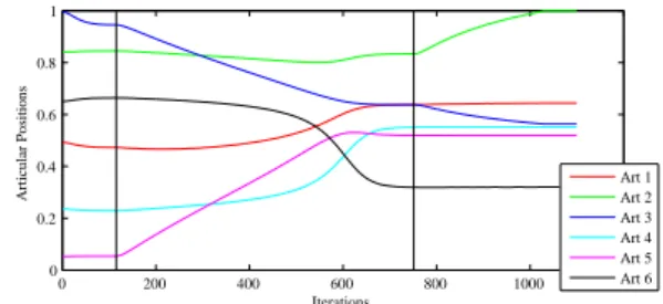
0 200 400 600 800 1000 1200 0 0.2 0.4 0.6 0.8 1 Iterations Articular Positions Art 1 Art 2 Art 3 Art 4 Art 5 Art 6
Fig. 3. Articular trajectories using the stack without any avoidance law. The second articulation (z-motion of the camera) reaches its limit during the execution of the third task (task ez). (each vertical line
corresponds to the addition of a new task in the stack.)
The robot lower and upper joint limits for each axis i
are denoted ¯qi
minand ¯qimax. The robot configuration q is
acceptable if, for all i, qi∈ [¯qmini , ¯qmaxi ], where ¯qmini =
¯
qimin+ ρ¯qi, ¯qmaxi = ¯qmaxi − ρ¯qi, ¯qi = ¯qimax− ¯qimin is the length of the domain of the articulation i, and
ρ is a tuning parameter, in [0, 1/2] (typically, ρ = 0.1).
¯
qmini and ¯qmaxi are activation threshold. In the acceptable
interval, the avoidance force should be zero. The cost function is thus given by (see Fig. 2) [4]:
V(q) =1 2 n X i=1 δi2 ∆¯qi (26) where δi = qi− ¯qmini , qi− ¯qmaxi , 0, if qi< ¯qmini if qi> ¯qmaxi else C. Results
When the three first tasks are completed, the robot is in one corner of its available domain, near the joint limit corresponding to the motion along the optical axis. Using the four visual tasks presented above into a classical servo fails because of the too large displacement between initial and desired position and the closeness of the joint limits. We present quickly the results obtained with the stack alone (13), then with the stack using the simple avoidance law (16). Without any avoidance, the robot reaches its joint limit quickly, during the third task, while DOF remain available (see Fig.3). This joint limit is avoided using the simple GPM. Instead of going back along the optical-axis, the robot moves along its x and
y axes and completes the task. Therefore, the joint limit
can not be avoided when the stack is full, because no DOF are available to project the gradient. The execution failed during the execution of the last elementary task
eR (see Fig. 4).
We present now the results obtained with the complete method (see Fig. 5). During the execution of the last task, the stack controller detects that the joint limit will be reached on axis 2. The controller chooses to remove the
task ez, and the task eRis completed using the obtained
DOF. The task ez is then put back in the stack, and the
0 200 400 600 800 1000 1200 1400 0 0.2 0.4 0.6 0.8 1 Iterations Articular Positions Art 1 Art 2 Art 3 Art 4 Art 5 Art 6
Fig. 4. Articular trajectories using the stack with the GPM but without stack controller. The limit is avoided during the execution of the third task (ez) by moving along the axis 1. The robot reaches its joint limit
during the last task, when no DOF are available any more.
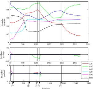
0 500 1000 1500 2000 2500 3000 0 0.2 0.4 0.6 0.8 1 Articular Positions 0 500 1000 1500 2000 2500 3000 −0.1 0 0.1 Avoidance gradient 0 500 1500 2000 2500 3000 −0.1 0 0.1 Iterations Projected gradient Art 1 Art 2 Art 3 Art 4 Art 5 Art 6 (2) (1) (3)(4) (5)
Fig. 5. During the execution of the first task (before event (1)), the avoidance is activated. Since there are many DOF left, the gradient is almost unchanged by the projection operator (gradient and projected gradient are almost equal). The joint limit avoidance is then activated during the task 3 (after event (2)). The obstacle is avoided using the DOF available. Not many DOF remain free, so the gradient is strongly modified by the projection. Therefore, the joint limit is avoided. During the last task, the obstacle can not be avoided (event (3)). No DOF are available, the projected gradient is thus null even if the gradient is not null. The task ezis removed from the stack (event (4)). The obstacle
is avoided. The task ezis finally put back in the stack (event (5)). At
the end of the execution, the avoidance is activated once more, but no DOF are available. The projected gradient is null. Therefore, the robot can complete the task despite the closeness of the joint limit. The stack controller does not remove any task from the stack.
VI. CONCLUSION
In this paper, we proposed a new method to avoid undesirable configurations such as obstacles or joint limits. Far from the desired position, the robot is un-derconstrained, and the remaining DOF are used for avoidance. When not enough DOF are available, a stack controller has been designed to remove the elementary task from the stack which will free the most appropriate DOF for the avoidance. This control scheme has been validated on a 6-DOF robotic platform. The robot had to reach the desired position from a distant initial position. The classical servoing scheme drive the robot into its joint limits, but using the proposed method, the execution ended properly.
Further work is necessary to validate experimentally this approach when taking into account several additional constraints, such as occlusion, obstacle and joint limits avoidance simultaneously. The stack controller should
also be able to choose automatically which task to put in the stack without any a priori as supplied here. The robot will thus be able to choose which elementary task to use among a very large amount of possible tasks.
REFERENCES
[1] P. Baerlocher and R. Boulic. An inverse kinematic architecture enforcing an arbitrary number of strict priority levels. The Visual
Computer, 6(20), 2004.
[2] F. Chaumette. Potential problems of stability and convergence in image-based and position-based visual servoing. In D. Kriegman, G . Hager, and A.S. Morse, editors, The Confluence of Vision and
Control, pages 66–78. LNCIS Series, No 237, Springer-Verlag,
1998.
[3] F. Chaumette. Image moments: a general and useful set of features for visual servoing. IEEE Trans. on Robotics, 20(4):713–723, August 2004.
[4] F. Chaumette and E. Marchand. A redundancy-based iterative scheme for avoiding joint limits: Application to visual servoing.
IEEE Trans. on Robotics and Automation, 17(5):719–730,
Octo-bre 2001.
[5] G. Chesi, K. Hashimoto, D. Prattichizzo, and A. Vicino. A switching control law for keeping features in the field of view in eye-in-hand visual servoing. IEEE Int. Conf. on Robotics and
Automation (ICRA’03), 3:3929–3934, September 2003.
[6] N.J. Cowan, J.D. Weingarten, and D.E. Koditschek. Visual servoing via navigation functions. IEEE Trans. on Robotics and
Automation, 18(4):521– 533, August 2002.
[7] B. Espiau, F. Chaumette, and P. Rives. A new approach to visual servoing in robotics. IEEE Trans. on Robotics and Automation, 8(3):313–326, June 1992.
[8] N. R. Gans and S. A. Hutchinson. An experimental study of hybrid switched approaches to visual servoing. IEEE Int. Conf.
on Robotics and Automation (ICRA’03), 3:3061–3068, September
2003.
[9] G. D. Hager. Human-machine cooperative manipulation with vision-based motion constraints. Workshop on visual servoing,
IROS’02, October 2002.
[10] S. Hutchinson, G. Hager, and P. Corke. A tutorial on visual servo control. IEEE Trans. on Robotics and Automation, 12(5):651– 670, October 1996.
[11] A. Liegeois. Automatic supervisory control of the configuration and behavior of multibody mechanisms. IEEE Trans. on Systems,
Man and Cybernetics, 7(12):868–871, December 1977.
[12] E. Malis, F. Chaumette, and S. Boudet. 2 1/2 D visual servoing.
IEEE Trans. on Robotics and Automation, 15(2):238–250, April
1999.
[13] N. Mansard and F. Chaumette. Tasks sequencing for visual servoing. In IEEE/RSJ Int. Conf. on Intelligent Robots and
Systems (IROS’04), Sendai, Japan, November 2004.
[14] E. Marchand and G.-D. Hager. Dynamic sensor planning in visual servoing. In IEEE/RSJ Int. Conf. on Intelligent Robots
and Systems (IROS’98), volume 3, pages 1988–1993, Leuven,
Belgium, May 1998.
[15] Y. Mezouar and F. Chaumette. Path planning for robust image-based control. IEEE Trans. on Robotics and Automation,
18(4):534–549, August 2002.
[16] L. Peterson, D. Austin, and D. Kragic. High-level control of a mobile manipulator for door opening. IEEE Int. Conf. on Robotics
and Automation (ICRA’03), 3:2333–2338, September 2003.
[17] R. Pissard-Gibolet and P. Rives. Applying visual servoing techniques to control a mobile hand-eye system. IEEE Int. Conf.
on Robotics and Automation (ICRA’96), pages 166 – 171, May
1996.
[18] C. Samson, M. Le Borgne, and B. Espiau. Robot Control: the Task
Function Approach. Clarendon Press, Oxford, United Kingdom,
1991.
[19] B. Siciliano and J-J. Slotine. A general framework for managing multiple tasks in highly redundant robotic systems. In ICAR’91, pages 1211 – 1216, 1991.
[20] P. Soueres, V. Cadenat, and M. Djeddou. Dynamical sequence of multi-sensor based tasks for mobile robots navigation. 7th Symp.
on Robot Control (SYROCO’03), 2:423– 428, September 2002.
[21] O. Tahri and F. Chaumette. Image moment: generic descriptors for decoupled image-based visual servo. IEEE Int. Conf. on Robotics
and Automation (ICRA’04), April 2004.