HAL Id: hal-02547982
https://hal.archives-ouvertes.fr/hal-02547982
Submitted on 20 Apr 2020
HAL is a multi-disciplinary open access
archive for the deposit and dissemination of
sci-entific research documents, whether they are
pub-lished or not. The documents may come from
teaching and research institutions in France or
abroad, or from public or private research centers.
L’archive ouverte pluridisciplinaire HAL, est
destinée au dépôt et à la diffusion de documents
scientifiques de niveau recherche, publiés ou non,
émanant des établissements d’enseignement et de
recherche français ou étrangers, des laboratoires
publics ou privés.
Diego Kiedanski, Lauren Kuntz, Daniel Kofman
To cite this version:
Diego Kiedanski, Lauren Kuntz, Daniel Kofman. Benchmarks for Grid Flexibility Prediction:
En-abling Progress and Machine Learning Applications. International Conference on Learning
Repre-sentations Workshop: ”Tackling Climate Change with Machine Learning”, Apr 2020, Addis Ababaa,
Ethiopia. �hal-02547982�
B
ENCHMARKS FOR
G
RID
F
LEXIBILITY
P
REDICTION
:
E
NABLING
P
ROGRESS AND
M
ACHINE
L
EARNING
A
P
-PLICATIONS
Diego Kiedanski Lauren Kuntz Daniel Kofman
ABSTRACT
Decarbonizing the grid is recognized worldwide as one of the objectives for the next decades. Its success depends on our ability to massively deploy renewable resources, but to fully benefit from those, grid flexibility is needed. In this pa-per we put forward the design of a benchmark that will allow for the systematic measurement of demand response programs’ effectiveness, information that we do not currently have. Furthermore, we explain how the proposed benchmark will facilitate the use of Machine Learning techniques in grid flexibility applications.
1
INTRODUCTION
Demand response (DR) or grid flexibility (GF) encompasses the ability of end-customers to change their energy consumption in response to incentives, with the goal of improving the operation of the power grid. Typically, examples of DR include Time-of-Use tariffs, where consumers are offered different electricity prices at different times of the day (such having a cheaper electricity price during the night) or direct control of appliances such as water heaters by a central utility (without impacting the comfort of users).
1.1 MOTIVATION
Climate change is one of the biggest challenges ever faced by humanity. A recent book by Hawken (2017), compiles a list of techniques to help reverse climate change. Regarding grid flexibility, it mentions that the impact was not measured because the system is too complex to properly assess its benefits. Even though demand response is a vital tool for enabling the energy transition and the deployment of renewable resources, there seems to be no reliable and reproducible measure for the performance of such techniques.
Consider a small low voltage (LV) grid1with several households and no demand response program
in place. One could wonder what is the most effective (in terms of consumption change and cost of implementation) DR program that could be deployed. Should we encourage users to install smart appliances and a Home Energy Management System (HEMS)? If there are appliances, is it better to use dynamic pricing, create local energy markets or directly pay users to gain the control of their HEMS? Would the results change if there were electric vehicles in every household?
1.2 THE ROLE OF BENCHMARKS
Standardized datasets and benchmarks exist and are important in many STEM areas. For example, in the artificial intelligence community, image recognition is arguably one of the most developed areas of research. There are many reasons for this, but the fact that anyone can develop a machine learning algorithm, evaluate it on a dataset such as MNIST (Deng, 2012) and know whether the implementation is working as expected is a major benefit. In particular, for the MNIST dataset there are leaderboards that contain the performance of several algorithms2. Even though the superior performance of one algorithm over another one for a specific dataset should not be sufficient to
1A LV grid is defined as the power grid behind the last Medium Voltage to Low Voltage transformer. The
vast majority of households are connected in a LV grid.
claim that one is better than the other, such comparison across different datasets might be a good indicator. Benchmarks are not exclusive of the Image Recognition community. Indeed, examples in other areas include: community detection in graphs (Lancichinetti et al., 2008) and natural language processing (Wang et al., 2019). Even in the power system community, the IEEE X-BUS systems (Kersting, 1991), (IEEE, 1979) provide benchmarking capabilities for some applications, but not for DR. In addition, Pecan Street (Smith, 2009) offers some benchmarking capabilities as a service. 1.3 BENCHMARK SPECIFICATION
Drawing a parallelism with the image processing community: the definition of an image is clear. It is a 3 dimensional matrix where each entry represents one of the RGB values of a pixel (for coloured images). Once everyone agreed in what an image is, many benchmarks (datasets) could be designed to solve different tasks: images with text, with objects, with faces, etc. There is not a clear analogous definition of what an “image“ is in Smart Grids, in particular for DR applications. In this section we take the first steps towards a definition that will enable the systematic treatment of DR programs. The requirements can be divided into four categories:
1. Energy Generation. 2. Power Grid Specification.
3. Consumer Specification. 4. Performance Metrics.
A brief description of each one of them can be found below, and we provide a longer description in the Appendix.
Energy Generation The amount of produced energy available for consumption, its sources and their respective location in the grid should be key components of a demand response benchmark. In particular, the information of how much renewable energy is available at each point in time will be needed for measuring DR performance as the ability to match consumption and renewable generation. Another piece of information that might be relevant consists on weather information such as temperature and cloud cover. That kind of information will be needed in more precise studies dealing with seasonal effects of demand response and its correlation to meteorological effects. This could also be relevant for the Consumer Specification.
Power Grid Specification The power grid can be seen as a graph, where edges are transmission lines and loads as well as generators are connected at the nodes. A detailed specification of the physical characteristics of each component will be required to produce realistic simulations. Formats already exist to provide detailed information about the grid topology and a well designed benchmark should reuse already established specifications. One such example is OpenDSS (Model & Element)
3.
Consumer Specification Consumers should be modeled in a manner that allows the users of the benchmark to derive the consumer change in behaviour in response to a change in the system. A simple way of doing so is by providing a set of appliances each consumer owns, together with their required usage. For example: non-flexible appliances such as TVs or lightbulbs should be paired with specific usage times, while washing machines or dishwashers (flexible appliances) could require only a start time and a completion deadline. The default price of electricity for consumers should be given. Those prices together with the list of appliances and their usage (and assuming that consumers act rationally to minimize their electricity bill), should provide enough information to derive each agent’s electricity consumption (actually, some extra details are required, see Appendix). Examples of possible problem formulations can be found in Paterakis et al. (2015), Chen et al. (2013) and Adika & Wang (2013).
Performance Metrics Having a standardized measure to evaluate demand response programs is critical to the idea of the benchmark and we believe it should be part of its specification. In this regard, measuring the mismatch between renewable generation and energy consumption4seems to
3OpenDSS is an electric power Distribution System Simulation 4
How much renewable energy needs to be curtailed and how much energy needs to be produced by tradi-tional generation sources when renewables are not sufficient
be a good choice, in contrast to the traditional peak reduction. Further discussion on this point can be found in Appendix B.5.
We conclude this section with a brief discussions on the limitations of our approach. Demand re-sponse is a complex problem that encompasses a wide range: from technical capabilities of the power grid to be controlled in real-time to patterns in human behaviour that modify how households react to incentives. It is then reasonable to question the validity of results obtained by an approach that draws mainly from the engineering nature of the problem, as we propose. We motivate our approach as follows. First, the capability of comparing the performance of different DR programs applied to the same reality will enhance our understanding of what it is required to properly imple-ment them, even if such knowledge deals only with the technological aspects of DR. Secondly, to avoid adding biases about human behaviour to the benchmark, we restrict ourselves to the case in which all flexibility and change in consumption is enabled by smart appliances and does not require the active participation of household owners.
2
MACHINE
LEARNING APPLICATIONS
Once benchmarks are established, there are many possible machine learning (ML) applications. Here, we provide two ideas on how ML can be useful in applications related to predicting the value of the unmet renewable energy generation. Observe that from the specification presented in Subsection 1.3, it is possible to build a massive number of datasets by creating variations of the topology, the appliances available, the number of consumers, etc.
2.1 DEEP LEARNING ON THE RAW DATASET
With computational effort, it should be possible to approximate, for each of the aforementioned datasets, the default aggregated consumption without any DR. It should also be possible to com-pute the optimal flexibility profile that a centralized entity could achieve it it had control of all the appliances available. This would yield a labeled training set where each data point is one of the benchmarks, and the label is the optimal profile that can be obtained. We envision that a deep learn-ing algorithm could be trained to predict such performance by identifylearn-ing the relevant features in the benchmark. For example, it might be that the total count of batteries plus water heaters with their corresponding electricity price is a good predictor of the net grid flexibility. In that case, the algo-rithm could learn the best predictors of performance and then be used to predict the grid flexibility capabilities of other regions of the grid. This could also be seen as a problem of Transfer Learning. 2.2 REINFORCEMENTLEARNING
It is very likely that implementing and simulating a real-time HEMS will require solving large mixed integer optimization problems. Doing so for large grids and lengthy time horizons can prove intractable. In this regards, reinforcement learning (but other techniques too) could be used to re-place the computationally expensive decision process faced by each agent. This could provide an opportunity to evaluate ML for real time-control. Even closer to demand response, reinforcement learning could be applied to learn a model of how agents change their behaviour from their default consumption profile to a different one in the presence of a DR program. This can be used to dis-cover and quickly test DR techniques in a variety of scenarios. Under ideal conditions, such tests could be used as a first step, followed by a through evaluation of the most promising techniques in comprehensive simulations of the benchmark.
3
CONCLUSIONS
In this paper we propose the design of a benchmark for demand response applications that will enable a systematic measurement of the grid flexibility available in different region of the grid. These measurements are crucial in the deployment of demand response programs, without which, the massive deployment of renewable resources and the decarbonization of the power system will be hindered. Together with a specification of such benchmark, we provide reader with two potential application of AI: predicting the maximum grid flexibility that could be achieved and learning how consumers will react to new demand response techniques.
REFERENCES
Christopher O Adika and Lingfeng Wang. Autonomous appliance scheduling for household energy management. IEEE transactions on smart grid, 5(2):673–682, 2013.
Xiaodao Chen, Tongquan Wei, and Shiyan Hu. Uncertainty-aware household appliance scheduling considering dynamic electricity pricing in smart home. IEEE Transactions on Smart Grid, 4(2): 932–941, 2013.
L. Deng. The mnist database of handwritten digit images for machine learning research [best of the web]. IEEE Signal Processing Magazine, 29(6):141–142, Nov 2012. ISSN 1558-0792. doi: 10.1109/MSP.2012.2211477.
Paul Hawken. Drawdown: The most comprehensive plan ever proposed to reverse global warming. Penguin, 2017.
IEEE. Ieee reliability test system. IEEE Transactions on Power Apparatus and Systems, PAS-98(6): 2047–2054, Nov 1979. ISSN 0018-9510. doi: 10.1109/TPAS.1979.319398.
William H Kersting. Radial distribution test feeders. IEEE Transactions on Power Systems, 6(3): 975–985, 1991.
Diego Kiedanski, Ariel Orda, and Daniel Kofman. The effect of ramp constraints on coalitional storage games. In Proceedings of the Tenth ACM International Conference on Future Energy Systems, e-Energy ’19, pp. 226–238, New York, NY, USA, 2019. Association for Computing Machinery. ISBN 9781450366717. doi: 10.1145/3307772.3328300. URL https://doi. org/10.1145/3307772.3328300.
Diego Kiedanski, Ariel Orda, and Daniel Kofman. Discrete and stochastic coalitional stor-age games. In leventh ACM International Conference on Future Energy Systems (ACM e-Energy), Melbourne, Australia, 2020. doi: 10.1145/1122445.1122456. URL https://hal. archives-ouvertes.fr/hal-02547962.
Andrea Lancichinetti, Santo Fortunato, and Filippo Radicchi. Benchmark graphs for testing commu-nity detection algorithms. Phys. Rev. E, 78:046110, Oct 2008. doi: 10.1103/PhysRevE.78.046110. URL https://link.aps.org/doi/10.1103/PhysRevE.78.046110.
Joel Mathias, Rim Kaddah, A Buic, and Sean Meyn. Smart fridge/dumb grid? demand dispatch for the power grid of 2020. In 2016 49th Hawaii International Conference on System Sciences (HICSS), pp. 2498–2507. IEEE, 2016.
OP Model and OpenDSS Storage Element. Opendss manual. EPRI,[Online] Available at: http://sourceforge. net/apps/mediawiki/electricdss/index. php.
N. G. Paterakis, O. Erdinc¸, A. G. Bakirtzis, and J. P. S. Catal˜ao. Optimal household appli-ances scheduling under day-ahead pricing and load-shaping demand response strategies. IEEE Transactions on Industrial Informatics, 11(6):1509–1519, Dec 2015. ISSN 1941-0050. doi: 10.1109/TII.2015.2438534.
Christopher Alan Smith. The Pecan Street Project: developing the electric utility system of the future. PhD thesis, Citeseer, 2009. URL https://www.pecanstreet.org/.
Alex Wang, Amanpreet Singh, Julian Michael, Felix Hill, Omer Levy, and Samuel R. Bowman. GLUE: A multi-task benchmark and analysis platform for natural language understanding. In 7th International Conference on Learning Representations, ICLR 2019, New Orleans, LA, USA, May 6-9, 2019, 2019. URL https://openreview.net/forum?id=rJ4km2R5t7.
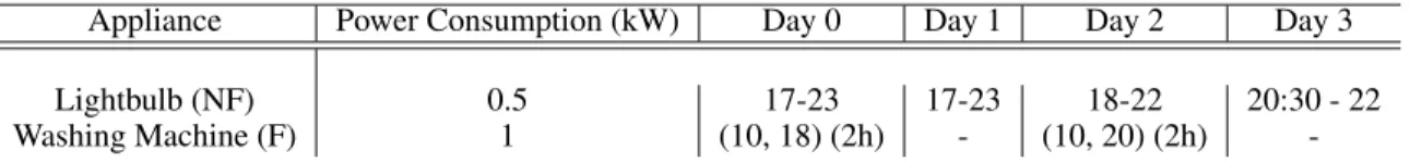
Appliance Power Consumption (kW) Day 0 Day 1 Day 2 Day 3 Lightbulb (NF) 0.5 17-23 17-23 18-22 20:30 - 22 Washing Machine (F) 1 (10, 18) (2h) - (10, 20) (2h)
-Table 1: Appliance usage and power consumption as specified in a possible benchmark
A
A
SIMPLE EXAMPLEIn this section we provide a minimal example of how a consumer can be modeled from the bench-mark data. The appliance usage of one consumer, Ana, is provided in Table 1. Consumption times are specified in hours, the minimal unit of time. Lightbulbs are non-flexible appliances and the pro-vided range is exactly the period of time in which they will be on. On the other hand, the washing machine is flexible, and the first pair of brackets defines the interval in which the consumer finds acceptable that the machine operates. The second pair of brackets indicates for how long it should (continuously) run once it starts. The electricity rate follows a Time-of-Use tariff with a cost of 15 ¢/ kWh between 14h - 22h and 10 ¢/ kWh at other times. The default consumption of Ana during Day 0 can be found by solving Optimization Problem as defined in equation 1a. In it, ctdenotes the
energy consumption at time-slot t, ltis a binary variable that indicates whether the light bulb is on
or off at time-slot t and ztplays the same role for the washing machine. wtis an auxiliary variable
that decides when the washing machine will turn on. An optimal solution can be found by turning the washing machine before the change in price (for example, w10= 1) at a total cost of 23.5¢.
This example contains many implicit assumptions such as the time resolution and the time horizon used to solve the optimization problem. In the next Appendix there is a more thorough discussion on some of these assumptions.
minimize lt, wt 22 X t=14 15ct+ X t∈[1,13]∪{23} 10ct (1a) subject to ct= 0.5lt+ ztt = 1, . . . , 24, (1b) z = wW, (1c) 17 X t=14 wt= 1, (1d) wt= 0 t ∈ [0, 13] ∪ [18, 23], (1e) lt= 0 t ∈ [1, 16] ∪ [24], (1f) lt= 1 t ∈ [17, 23], (1g) w, z ∈ {0, 1}T (1h) W = 1 1 0 0 . . . 0 0 1 1 0 . . . 0 .. . . . ... 0 0 . . . 0 1 1 (2)
B
BENCHMARK SPECIFICATION CONT.
In this section we provide some additional discussion on the decision space of the benchmark. B.1 DETAIL LEVEL OF THE APPLIANCES
One key question in the design of the dataset is how realistic should the model of the appliances be. A very detailed description might make the benchmark too complicated for normal use whereas
a too simplistic model might force users to add their own modifications, defeating the purpose of the benchmark altogether. For example, consider the case of battery storage. A description of such storage should include the maximum battery capacity, the minimum battery capacity and the maximum and minimum charging and discharging power. It should most likely also include the charging and discharging efficiencies. But should it consider a non-constant efficiency that depends on the state of charge? Should it include the likelihood of a random discharge? The most useful level of detail probably lies in the middle, where most researchers can feel comfortable about the realism of the model. Finally, to enable power flow calculations using the benchmark, appliances should include their power factor.
B.2 MODULARITY
Not every project calls for the same level of detail. For example, in Mathias et al. (2016) the authors propose a distributed algorithm for controlling swimming pools. For such application, the need to deal with extra appliances (appart from swimming pools) might be seen as a reason not to use the benchmark (“it is too much for our problem“). A second example could be modeling the shared investment in storage by a collective of users without one, such as the one proposed in Kiedanski et al. (2019), Kiedanski et al. (2020). In that particular application, only the net load might be required and having to deal with specific appliances might be seen as a drawback. This will be a key factor in the adoption of the benchmark: it should not be overly simplistic nor overly detailed for most users.
In that regard, the benchmark should be designed in a way that allows for some of its parts to be en-capsulated and treated as black boxes if desired. In particular, for a deterministic dataset, the default operation (obtained in a pre-specified manner) can be distributed together with the original data. For the use-case of the distributed control of the pools, the interested user can fix all the appliances to behave as in the default scenario and deal only with the flexibility of the pools. By doing so, he/she can assess in a realistic scenario the added benefit of the distributed control mechanisms with respect to the normal performance.
B.3 GRANULARITY
Some applications closer to the physical power grid might require load samples every minute, while testing complicated game theoretical models might only allow for sampling at periods of 30 min-utes or greater. An important quality regarding time granularity is to find a standardized way of aggregating time-slots. That way, if the benchmark is distributed at the 5 minute level, but an ap-plication requires data sampled hourly, it will be possible for them to aggregate it for their use and dis-aggregate it later, producing results in the standard format.
This seems to indicate that the smaller the granularity, the better, as we can always go to coarser load profiles. Nevertheless, the computational complexity produced by a dataset sampled every milliseconds will not provide added benefits to the DR community. The sweet spot seems to be around 1 or 5 minutes, but is up for discussion.
B.4 DEFAULT OPERATION
So far, we have discussed how to design the dataset and what information should be included in it. Unfortunately, this is still not sufficient to provide a reliable and reproducible benchmark. Central to the idea of a benchmark is the idea of comparing the performance of one technique to another one. This calls for a “default operational mode“ (DOM), i.e., the behaviour of the system when no DR program is applied to it. Clearly, this default mode should be uniquely specified in the data. We want to point out that this is not trivial to achieve and that extra specification will be required to guarantee the existence of a unique DOM. The simplest approach to obtain a DOM would be to solve an optimization problem for each household that outputs a schedule of all the appliances, such that the total cost payed for electricity is minimized. We shall refer to this solution as the Default with Perfect Information (DwPI). There are two main problems with the DwPI. First, it can be computationally impossible to find. Consider a dataset containing samples with a resolution of 1 minute and a horizon of 1 year: there are more than half a million time-slots, each one of them with several discrete variables. Secondly, the result obtained will not be representative of a real settings in
which agents have to forecast their load and even maybe their prices. One way to solve this problem is to use a forecast of the load and a rolling horizon Model Predictive Control technique to obtain the DOM of a consumer. If the length of the horizon and the forecasting technique are pre-specified, then a unique solution can be obtained5: the Default with Forecast (DwF).6
B.5 MEASURING GRID FLEXIBILITY
In a power grid where all the generation is dispatchable7, peak reduction has been traditionally the
objective of demand response programs. This was motivated by the fact that the most complex task was to satisfy the higher peaks of demand. With the introduction of non-dispatchable generation such as solar and wind, matching the produced energy with the consumption becomes ones of the most important problems to solve, as there is no benefit in installing non-dispatchable loads if there will be no consumption when there is generation. We believe that the matching between generation and consumption should be a central measure of grid flexibility. To obtain a concrete measure of it, we can define grid flexibility as the integral of the difference between renewable production and consumption. We can further distinguish between curtailment (generation is larger than consump-tion) and unmet demand (which required extra generation capabilities to be dispatched). The later is arguably worse than the former, so we can envision a metric defined as the weighted average of the two quantities, with a higher emphasis on the unmet demand.
B.6 VALUATION OF LOAD SHEDDING
One of the traditional mechanisms for DR is load shedding. Properly modeling such a mechanism requires the valuation of agents for not consuming their required energy. For flexible loads, this value can be obtained by shifting around the load and trying to obtain a new, feasible allocation, possibly at a higher cost. For inflexible loads, or when the flexibility is not sufficient, the procedure described above will not provide the required answer. Instead, the dataset should specify an external valuation of that quantity, i.e, at what price will each household turn off their inflexible appliances. This value is intrinsically personal and depends in the socioeconomically situation of each agent. For example, a household in a rich neighbourhood might be willing to pay more to keep their swimming pool warm than a poor family will be willing to pay to keep their heating on during winter. There is no clear way to obtain a representative valuation for this. Some sort of valuation belonging to a specific family of functions could be assumed (lets say quadratic with sampled coefficients), but it will likely result in biased results towards DR techniques with similar assumptions (positively or negatively). The other alternative would be to limit the scope of the benchmark and decide that such demand response programs are not included, which in principle is undesirable given the important role of such mechanisms.
5If the solution is not unique, additional information will have to be provided to select among them. 6The forecasting technique should be deterministic and clearly specified for border cases.
7