Recurrent neural models and related problems in natural language processing

(1)

Universit´e de Montr´eal

Recurrent Neural Models and Related Problems in Natural Language Processing

par Saizheng Zhang

Département d’informatique et de recherche opérationnelle Faculté des arts et des sciences

Thèse présentée à la Faculté des arts et des sciences en vue de l’obtention du grade de Philosophiæ Doctor (Ph.D.)

en informatique

avril, 2019

c

(2)

Résumé

Le réseau de neurones récurrent (RNN) est l’un des plus puissants modèles d’ap-prentissage automatique spécialisés dans la capture des variations temporelles et des dépendances de données séquentielles. Grâce à la résurgence de l’apprentissage en profondeur au cours de la dernière décennie, de nombreuses structures RNN innovantes ont été inventées et appliquées à divers problèmes pratiques, en par-ticulier dans le domaine du traitement automatique du langage naturel (TALN). Cette thèse suit une direction similaire, dans laquelle nous proposons de nouvelles perspectives sur les propriétés structurelles des RNN et sur la manière dont les mo-dèles RNN récemment proposés peuvent stimuler le developpement de nouveaux problèmes ouverts en TALN.

Cette thèse se compose de deux parties: l’analyse de modèle et le traitement de nouveaux problèmes ouverts. Dans la première partie, nous explorons deux aspects importants des RNN: l’architecture de leurs connexions et les opérations de base dans leurs fonctions de transition. Plus précisément, dans le premier article, nous définissons plusieurs mesures rigoureuses pour évaluer la complexité architecturale de toute architecture récurrente donnée, quelle que soit la topologie du réseau. Des expériences approfondies sur ces mesures démontrent à la fois la validité théorique de celles-ci, et l’importance de guider la conception des architectures RNN. Dans le deuxième article, nous proposons un nouveau module permettant de combiner plusieurs flux d’informations de manière multiplicative dans les fonctions de tran-sition de base des RNN. Il a été démontré empiriquement que les RNN équipés du nouveau module possédaient de meilleures propriétés de gradient et des capacités de généralisation plus grandes sans coûts de calcul et de mémoire supplémentaires. La deuxième partie se concentre sur deux problèmes non résolus de la TALN: comment effectuer un raisonnement avancé à sauts multiples en compréhension de texte machine, et comment incorporer des traits de personnalité dans des systèmes conversationnels. Nous recueillons deux ensembles de données à grande échelle, dans le but de motiver les progrès méthodologiques sur ces deux problèmes. Sp´ e-cifiquement, dans le troisième article, nous introduisons l’ensemble de données sc HotpotQA qui contient plus de 113 000 paires question-réponse basées sur Wiki-pedia. La plupart des questions de HotpotQA ne peuvent résolues que par un raisonnement multi-saut précis sur plusieurs documents. Les faits à l’appui n´ eces-saires au raisonnement sont également fournis pour aider le modèle à établir des prédictions explicables. Le quatrième article aborde le problème du manque de personnalité des chatbots. Le jeu de donn´_{ees persona-chat que nous proposons}

(3)

encourage des conversations plus engageantes et cohérentes en conditionnant la personnalité des membres en conversation sur des personnages spécifiques. Nous montrons des modèles de base entraˆın´_{es sur persona-chat sont capables} d’ex-primer des personnalités cohérentes et de réagir de manière plus captivante en se concentrant sur leurs propres personnages ainsi que ceux de leurs interlocuteurs.

Mots clés: réseaux de neurones récurrents, apprentissage profond, traitement automatique du langage naturel, compréhension en lecture, système de dialogue

(4)

Summary

The recurrent neural network (RNN) is one of the most powerful machine learn-ing models specialized in capturlearn-ing temporal variations and dependencies of sequen-tial data. Thanks to the resurgence of deep learning during the past decade, we have witnessed plenty of novel RNN structures being invented and applied to vari-ous practical problems especially in the field of natural language processing (NLP). This thesis follows a similar direction, in which we offer new insights about RNNs’ structural properties and how the recently proposed RNN models may stimulate the formation of new open problems in NLP.

The scope of this thesis is divided into two parts: model analysis and new open problems. In the first part, we explore two important aspects of RNNs: their connecting architectures and basic operations in their transition functions. Specif-ically, in the first article, we define several rigorous measurements for evaluating the architectural complexity of any given recurrent architecture with arbitrary net-work topology. Thoroughgoing experiments on these measurements demonstrate their theoretical validity and utility of guiding the RNN architecture design. In the second article, we propose a novel module to combine different information flows multiplicatively in RNNs’ basic transition functions. RNNs equipped with the new module are empirically showed to have better gradient properties and stronger generalization capacities without extra computational and memory cost.

The second part focuses on two open problems in NLP: how to perform advanced multi-hop reasoning in machine reading comprehension and how to encode person-alities into chitchat dialogue systems. We collect two different large scale datasets aiming to motivate the methodological progress on these two problems. Particu-larly, in the third article we introduce HotpotQA dataset containing over 113k Wikipedia based question-answer pairs. Most of the questions in HotpotQA are answerable only through accurate multi-hop reasoning over multiple documents. Supporting facts required for reasoning are also provided to help the model to make explainable predictions. The fourth article tackles the problem of the lack of personality in chatbots. The proposed persona-chat dataset encourages more engaging and consistent conversations by forcing dialog partners conditioning on given personas. We show that baseline models trained on persona-chat are able to express consistent personalities and to respond in more captivating ways by con-centrating on personas of both themselves and other interlocutors.

(5)

(6)

List of Figures

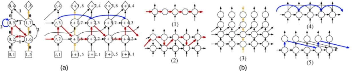
4.1 (a) An example of an RNN’s Gc and Gun. Vin is denoted by square, Vhid is denoted by circle and Vout is denoted by diamond. In Gc, the number on each edge is its corresponding σ. The longest path is colored in red. The longest input-output path is colored in yellow and the shortest path is colored blue. The value of three measures are dr = 3₂, df = 3.5 and s = 2. (b) 5 more examples. (1) and (2) have dr = 2,3₂, (3) has df = 5, (4) and (5) has s = 2,3₂. . . 44 4.2 (a) The architectures for sh, st, bu and td, with their (dr, df) equal to

(1, 2), (1, 3), (1, 3) and (2, 3), respectively. The longest path in td are colored in red. (b) The 9 architectures denoted by their (df, dr) with

dr = 1, 2, 3 and df = 2, 3, 4. We only plot the hidden states within 1 time

step (which also have a period of 1) in both (a) and (b). . . 49 4.3 (a) Various architectures that we consider in Section 4.4.4. From top to

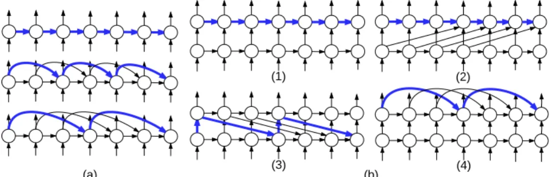
bottom are baseline s = 1, and s = 2, s = 3. (b) Proposed architectures that we consider in Section 4.4.5 where we take k = 3 as an example. The shortest paths in (a) and (b) that correspond to the recurrent skip coefficients are colored in blue. . . 52 6.1 (a) Curves of log-L2-norm of gradients for lin-RNN (blue) and

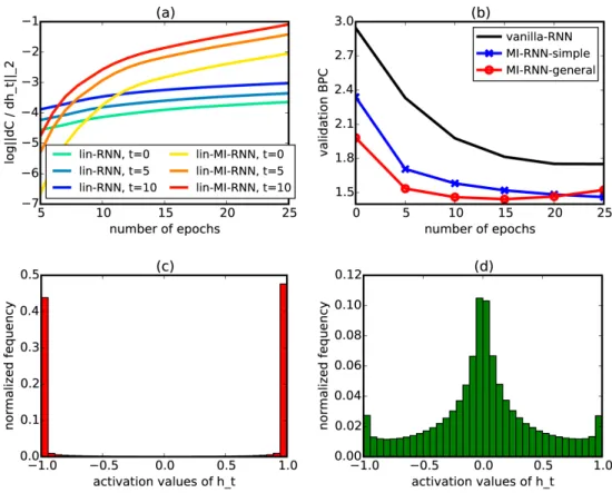
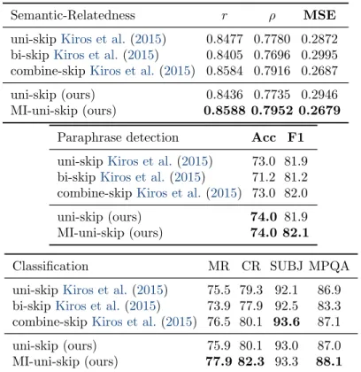
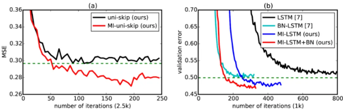
lin-MI-RNN (orange). Time gradually changes from {1, 5, 10}. (b) Valida-tion BPC curves for vanilla-RNN, MI-RNN-simple using Eq. 6.2, and MI-RNN-general using Eq. 6.4. (c) Histogram of vanilla-RNN’s hidden activations over the validation set, most activations are saturated. (d) Histogram of MI-RNN’s hidden activations over the validation set, most activations are not saturated. . . 68 6.2 (a) MSE curves of uni-skip (ours) and MI-uni-skip (ours) on semantic

relatedness task on SICK dataset. MI-uni-skip significantly outperforms baseline uni-skip. (b) Validation error curves on attentive reader models. There is a clear margin between models with and without MI. . . 74 8.1 _{An example of the multi-hop questions in HotpotQA. We also}

highlight the supporting facts in blue italics, which are also part of the dataset. . . 82 8.2 Screenshot of our worker interface on Amazon Mechanical Turk. . . 87

(11)

8.3 _{Types of questions covered in HotpotQA. Question types are} ex-tracted heuristically, starting at question words or prepositions pre-ceding them. Empty colored blocks indicate suffixes that are too rare to show individually. See main text for more details. . . 91 8.4 Our model architecture. Strong supervision over supporting facts is

(12)

List of Tables

4.1 Test BPCs of sh, st, bu, td for tanh RNNs and LSTMs. . . 49 4.2 Test BPCs of tanh RNNs with recurrent depth dr = 1, 2, 3 and

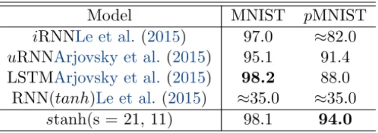
feedfor-ward depth df = 2, 3, 4 respectively. . . 50 4.3 Test accuracies with different s for tanh RNN and LSTM in MNIST/pMNIST. 52 4.4 our best model compared to previous results on MNIST/pMNIST. . . . 53 4.5 Test accuracies for architectures (1), (2), (3) and (4) for tanh RNN on

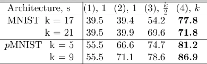
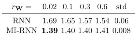
MNIST/pMNIST. . . 54 6.1 Test BPCs and the standard deviation of models with different scales of

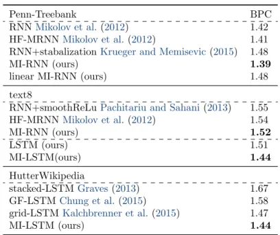
weight initializations. . . 69 6.2 Top: test BPCs on character level Penn-Treebank dataset. Middle: test

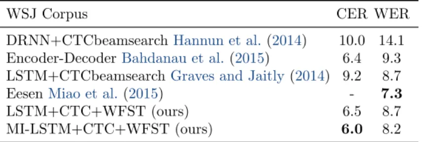
BPCs on character level text8 dataset. Bottom: test BPCs on character level Hutter Prize Wikipedia dataset. . . 70 6.3 Test CERs and WERs on WSJ corpus. . . 71 6.4 Skip-thought+MI on Semantic-Relatedness task (top), Paraphrase

De-tection task (middle) and four different classification tasks (bottom). . . 73 6.5 Multiplicative Integration (with batch normalization) on Teaching

Ma-chines to Read and Comprehend task. . . 75 8.1 Data split. The splits train-easy, train-medium, and train-hard are

combined for training. The distractor and full wiki settings use dif-ferent test sets so that the gold paragraphs in the full wiki test set remain unknown to any models. . . 88 8.2 Retrieval performance comparison on full wiki setting for train-medium,

dev and test with 1,000 random samples each. MAP and are in %. Mean Rank averages over retrieval ranks of two gold paragraphs. CorAns Rank refers to the rank of the gold paragraph containing the answer. . . 90 8.3 _{Types of answers in HotpotQA.} . . . 92

(13)

8.4 Types of multi-hop reasoning required to answer questions in the HotpotQA dev and test sets. We show in orange bold italics bridge entities if applicable, blue italics supporting facts from the paragraphs that connect directly to the question, and green bold

the answer in the paragraph or following the question. The remain-ing 8% are sremain-ingle-hop (6%) or unanswerable questions (2%) by our judgement. . . 93 8.5 Retrieval performance in the full wiki setting. Mean Rank is

aver-aged over the ranks of two gold paragraphs. . . 97 8.6 Main results: the performance of question answering and

support-ing fact prediction in the two benchmark settsupport-ings. We encourage researchers to report these metrics when evaluating their methods. . 97 8.7 Performance breakdown over different question types on the dev

set in the distractor setting. “Br” denotes questions collected using bridge entities, and “Cp” denotes comparison questions. . . 98 8.8 Ablation study of question answering performance on the dev set

in the distractor setting. “– sup fact” means removing strong su-pervision over supporting facts from our model. “– train-easy” and “– train-medium” means discarding the according data splits from training. “gold only” and “sup fact only” refer to using the gold paragraphs or the supporting facts as the only context input to the model. . . 99 8.9 Comparing baseline model performance with human performance on

1,000 random samples. “Human UB” stands for the upper bound on annotator performance on HotpotQA. For details please refer to the main body. . . 100 10.1 Example Personas (left) and their revised versions (right) from the

persona-chat dataset. The revised versions are designed to be characteristics that the same persona might have, which could be rephrases, generalizations or specializations. . . 108 10.2 Example dialog from the persona-chat dataset. Person 1 is given

their own persona (top left) at the beginning of the chat, but does not know the persona of Person 2, and vice-versa. They have to get to know each other during the conversation. . . 111 10.3 Evaluation of dialog utterance prediction with various

mod-els in three settings: without conditioning on a persona, conditioned on the speakers given persona (“Original Persona”), or a revised per-sona that does not have word overlap. . . 116

(14)

10.4 Evaluation of dialog utterance prediction with generative models in four settings: conditioned on the speakers persona (“self persona”), the dialogue partner’s persona (“their persona”), both or none. The personas are either the original source given to Turkers to condition the dialogue, or the revised personas that do not have word overlap. In the “no persona” setting, the models are equivalent, so we only report once. . . 116 10.5 Evaluation of dialog utterance prediction with ranking

mod-els using hits@1 in four settings: conditioned on the speakers sona (”self persona”), the dialogue partner’s persona (”their per-sona”), both or none. The personas are either the original source given to Turkers to condition the dialogue, or the rewritten personas that do not have word overlap, explaining the poor performance of IR in that case. . . 117 10.6 Human Evaluation of various persona-chat models, along with

a comparison to human performance, and Twitter and OpenSubti-tles based models (last 4 rows), standard deviation in parenthesis.

. . . 118 10.7 Profile Prediction. Error rates are given for predicting either the

persona of speaker 0 (Profile 0) or of speaker 1 (Profile 1) given the dialogue utterances of speaker 0 (PERSON 0) or speaker 1 (PER-SON 1). This is shown for dialogues between humans (PER(PER-SON 0) and either the KV Profile Memory model (“KV Profile”) which conditions on its own profile, or the KV Memory model (“KV w/o Profile”) which does not. . . 120 10.8 Profile Prediction By Dialog Length. Error rates are given for

predicting either the persona of speaker 0 (Profile 0) or of speaker 1 (Profile 1) given the dialogue utterances of speaker 0 (PERSON 0) or speaker 1 (PERSON 1). This is shown for dialogues between humans (PERSON 0) and the KV Profile Memory model averaged over the first N dialogue utterances from 100 conversations (where N is the “Dialogue Length”). The results show the accuracy of predicting the

persona improves in all cases as dialogue length increases. . . 120 10.9 Example dialog between a human (Person 1) and the OpenSubtitles

KV Memory Network model (Person 2). . . 122 10.10Example dialog between a human (Person 1) and the Seq2Seq model

(Person 2). . . 123 10.11Example dialog between a human (Person 1) and the Key-Value

Profile Memory Network with Self Persona. . . 124 10.12Example dialog between a human (Person 1) and the Generative

(15)

10.13Example dialog between a human (Person 1) and the Language Model trained on the OpenSubtitles 2018 dataset (does not use per-sona). . . 125 10.14Example dialog between a human (Person 1) and the Language

(16)

Acknowledgments

When I was reading Prof. Yoshua Bengio’s famous denoising autoencoder paper during my first undergraduate research project in 2011, I never thought that I will become his student in the following years. That paper strongly motivated me to find my research path towards neural networks (later well-known as deep learning) and finally drove me to pursue the Ph.D. under Yoshua’s supervision. As a researcher, I am impressed by Yoshua’s humility and curiosity to the unknown, although he is already a widely respected researcher in the field. As Yoshua’s student, I am very grateful for his insightful advices on my research, and more importantly, the freedom and patience given to me that allow me to explore my own research interests. A famous Chinese proverb says, “Give a man a fish and you feed him for a day; teach a man to fish and you feed him for a lifetime”. I would like to thank Yoshua to be my guide during the past five years, from whom the most precious thing I learned is not the machine learning knowledge, but how to be enthusiastic and stay brave when facing challenges.

I would like to thank my friend and co-author Yuhuai Wu from University of Toronto, with whom I wrote my first two NIPS papers which became the first part of this thesis. The days and nights spent with him chatting about research and life will become one of my most memorable experiences. I also would like to thank my friend Jake Zhao from New York University, from who I learned how to become ambitious and steadfast towards the goal that I am pursuing.

As a member of the big Mila family, I would like to thank all the friends I met there with whom I had a wonderful and unforgettable time: Zhouhan Lin, Yikang Shen, Harm de Vries, Laurent Dinh, Pengfei Liu, Mohammad Pezeshki, Min Lin, Jie Fu, Kyunghyun Cho, Alexandre de Br´ebisson, Sandeep Subramanian, Alex Lamb, Caglar Gulcehre, Orhan Firat, Taesup Kim, Anirudh Goyal, Benjamin Scellier, Asja Fischer, Junyoung Chung, Yuchen Lu, Guillaume Alain, Dong-hyun Lee, Chen Xing, Dmitriy Serdyuk, Li Yao, Gerry Che, Kyle Kastner, Iulian Vlad Serban, Jae Hyun Lim, Thomas Mesnard, Dzmitry Bahdanau, Akram Erraqabi, Nicolas Ballas, Prof. Aaron Courville and Prof. Roland Memisevic.

(17)

I am also very thankful to all my friends who are my collaborators outside Mila and offered me plentiful help in my research: Hongyuan Mei from John Hopkins University, Zhilin Yang and Prof. Ruslan Salakhutdinov from Carnegie Mellon University, Peng Qi from Stanford University, Jason Weston, Douwe Kiela, Arthur Szlam and Abdel-rahman Mohamed from Facebook AI Research, Xiang Zhang and Sungjin Ahn from Element AI, Xingdi Yuan, Tong Wang and Adam Trischler from Microsoft Research, Vinod Nair from Deepmind.

Finally, I would like to thank my parents and my wife Ying Zhang for their selfless support to my career. It was their love that helped me overcome all the obstacles during my Ph.D. life.

(18)

1

Introduction

With the resurgence of deep learning (DL) during the past decade, the recurrent neural network (RNN), as one of the critical members of neural network models, gradually drew attention from the machine learning research community because of its strong modeling capacity for sequential learning problems. Since 2014, RNNs soon took the center stage in a series of natural language processing (NLP) scenar-ios, including machine translation (Cho et al., 2014; Sutskever et al., 2014; Bah-danau et al., 2014), dialogue system (Vinyals and Le, 2015; Sordoni et al., 2015; Serban et al., 2016b) and machine reading comprehension (Hermann et al., 2015; Rajpurkar et al., 2016; Devlin et al., 2018). At the time, although the empirical success of the RNN was so significant that it reshaped the problem formulation and methodology in several subfields of NLP, relatively fewer research was conducted on the systematic understanding of RNNs’ architectural basics and computational fundamentals. This becomes the motivation of the first part of this thesis (Chapter 3 to Chapter 6 (Zhang et al., 2016; Wu et al., 2016)), in which we attempt to offer new insights on understanding the RNN’s architectural properties in a generic perspective as well as exploring new functional designs inside the RNN’s internal computational procedure. On the other hand, as the recently introduced advanced recurrent neural modules redefined the pipeline of NLP research, we are now able to explore new natural language scenarios which were infeasible before. The sec-ond part of this thesis (Chapter 7to Chapter10 (Yang et al., 2018a;Zhang et al., 2018)) is motivated by this trend, in which we dive deep into two open problems about multi-hop reasoning in machine reading comprehension and personality en-coding in dialogue systems. For both problems we collect new datasets and build corresponding baselines, hoping that our proposed testbed can promote the further research development in these two directions.

(19)

1.1 Architectural Analysis and New Structure

Design of RNNs

The original RNN (Rumelhart et al., 1985; Jordan, 1997; Elman, 1990), also known as “vanilla RNN”, has relatively simple structure in which a hidden state ht

at the current time step t is computed based on the current input xtand the

previ-ous hidden state ht−1via a set of linear transformations {W, U, b} and elementwise

nonlinearity σ:

ht = σ(Wxt+ Uht−1+ b). (1.1)

The vanilla RNN is also a single hidden layer RNN. In the following decades, various new connecting architectures were proposed based upon the vanilla RNN: Schmidhuber(1992);El Hihi and Bengio(1996) introduced different forms of stack-ing in RNNs where hidden layers are stacked on top of each other; Schuster and Paliwal(1997) proposed the bidirectional RNNs which conduct recurrent computa-tion in both forward and backward direccomputa-tion over the input sequence; Raiko et al. (2012);Graves (2013);Lin et al. (1996);El Hihi and Bengio(1996);Sutskever and Hinton (2010); Koutnik et al. (2014) explored the use of skip connections (short-cuts) among different hidden states and Hermans and Schrauwen (2013) proposed deep RNNs which are stacked RNNs with skip connections;Pascanu et al. (2013a) suggested adding more nonlinearities in RNNs’ transition functions to make RNNs “deeper” in the recurrent direction. Despite all the empirical success achieved so far, few of these research attempted to analyze RNN connecting architectures in a systematic way with generic and rigorous formulations. This leads to several drawbacks: (1) It is hard to quantitatively measure the complexity of different connecting architectures: even the concept of “depth” is not clear with current RNNs. (2) The lack of correct definition of connection architectures limits previ-ous researchers to only consider the simple “deep” RNNs while leaving vastly field of connecting variations unexplored. In the first paper (Chapter3and Chapter4), we attempt to rigorously analyze the connecting architectures of RNNs by introducing a generic graph-theoretic formulation under which we could further evaluate the architectural complexity of an RNN via three novel measures: recurrent depth, feed-forward depth, and recurrent skip coefficient. These measures reflect the fact that RNNs may undergoes multiple transformations not only feedforwardly (from input

(20)

to output within a time step) but also recurrently (across multiple time steps) in sophisticated ways. Compared with previous research, the recurrent depth can be viewed as a general extension of the work ofPascanu et al.(2013a), the feedforward depth can be considered as an accurate measure of the input-output nonlinearness for different stacked RNNs, and the recurrent skip coefficient plays the role of quan-tifying the complexity of various skip connections in RNNs. Notably, the recurrent skip coefficient is strongly related to vanishing/exploding gradient issues and helps dealing with long term dependency problems. Our experimental results on five different datasets validate the usefulness of the proposed definitions and measure-ments where they help answering the question of “What is the depth of an RNN?” under the generic scenario and are able to provide guidance for the design and inspection of new connecting architectures for particular learning tasks.

Besides the connecting architecture, another crucial structural aspect of the RNN is its transition function which describes the computational procedure associ-ated with each unit in the network. As we discussed before, the vanilla RNN adopts a very simple formulation in its transition function. Hochreiter and Schmidhuber (1997) invented the long short term memory (LSTM) in which they introduced the gating mechanism and memory cells, while Cho et al. (2014) further simplified the gating structures and proposed gated recurrent unit (GRU). Moreover, there is a recent resurgence of new structural designs for RNNs’ transition functions (Chung et al.,2015;Kalchbrenner et al.,2015;Jozefowicz et al.,2015), most of which are de-rived from vanilla RNNs, LSTMs or GRUs. Despite of their structural differences, they share a common computational building block either in their hidden-to-hidden or gating computations, described by the following equation:

φ(Wx + Uz + b). (1.2)

This computational building block serves as a combinator for integrating informa-tion flows from different sources x and z by an additive operainforma-tion “+”. Such additive operation are widely adopted in various state computations in RNNs (LSTMs and GRUs) including hidden state and gate/cell computations. In our second paper (Chapter 5 to Chapter 6), we consider an alternative in which the additive in-tegration is replaced by a multiplicative one. Specifically, we propose to use the

(21)

Hadamard product “” to fuse information from x and z:

φ(Wx Uz + b). (1.3)

We name the above information integration design as Multiplicative Integration (MI). MI naturally derives the gating effect between Wx and Uz where they dy-namically rescale each other. We empirically show that RNNs with MI enjoy better gradient properties due to such gating effect and most of the hidden units are non-saturated. From an engineering perspective, MI is one of the few improvements that directly touches the essential transition function of an RNN with (1) adaptability towards any recurrent models (e.g. LSTMs and GRUs), (2) no extra computational cost as it brings almost no extra parameters and (3) no extra engineering beyond implementing the RNN model itself. In Chapter 6 we will see that the general form of MI is by design performing at least as well as the standard RNN transition function. Our experimental results demonstrate that MI can provide a substantial performance boost over many of the existing RNN models.

1.2 Open Problems in Machine Reading

Comprehension and Dialogue System

One of the extraordinary intelligent skills of human is the ability of reasoning and inference over abstract symbols, especially natural languages. Such ability is also considered as a crucial step towards artificial general intelligence (AGI). Machine reading comprehension (MRC) and question answering (QA) tasks pro-vide measurable ways to verify the reasoning ability of intelligent machines, in which correctly answering the question requires the machine to perform sophisti-cated understanding and reasoning process over the given related natural language materials. Recently, the emergence of many large-scale QA datasets has sparked much progress in this direction. However, existing datasets have several limita-tions that hinder further advancements: (1) The most popular dataset SQuAD (Rajpurkar et al., 2016) only concentrates on testing single-step (or single-hop) reasoning ability where most of the questions can be addressed by matching the question with a single sentence in a single context paragraph. Machines trained on

(22)

this dataset end up with some keyword-matching like mechanisms and can hardly reason over a larger context. TriviaQA (Joshi et al., 2017b_{) and SearchQA} (Dunn et al., 2017) attempted to make the setting more challenging by collect-ing multiple documents as the context whilst most of the questions can still be answered by matching the question with a few nearby sentences in one single para-graph. (2) Datasets designed for multi-hop reasoning like WikiHop (Welbl et al., 2018a_{) and ComplexWebQ (}Talmor and Berant,2018) are constructed on exist-ing knowledge bases (KBs), which implies that they are constrained by the schema of the KBs used and therefore have very limited question-answer diversity. (3) Given a question, all the existing datasets provide the answer as the only distant supervision while the machine has no idea what supporting facts lead to that an-swer. This makes it difficult for explaining the machine’s prediction and tracing the underlying reasoning process. The HotpotQA1 _{dataset introduced in the third} paper (Chapter 7 to Chapter 8) tries to address the above challenges by forcing the question staying in natural language form, requiring reasoning over multiple facts in multiple documents (we name it as multi-hop reasoning), and not being constrained by existing KBs. It also explicitly highlights in-document supporting sentences for each question, which denote where the answer is actually derived, and thus help guiding the model to perform meaningful and explainable reasoning. Specifically, we collected the data via Amazon crowdsourcing service, where quali-fied workers are shown multiple context documents extracted from Wikipedia and asked explicitly to raise questions requiring reasoning over these documents. The entire data collection pipeline is carefully designed and we hope that this pipeline as a byproduct can also sheds light on future work in this direction. During the experiments, we show that the multi-hop reasoning questions in HotpotQA is challenging for the latest MRC systems and the supporting facts enable models to improve performance and make explainable predictions.

Question answering is in fact a single turn communication between the ques-tioner and the respondent. A more generic scenario is a conversation (dialogue) in which interlocutors conduct multiple turns of communication which require more complicated context understanding over the entire dialogue history. Despite the past success in NLP research, the communication between a human and a machine

1. The name comes from the first three authors’ arriving at the main idea during a discussion at a hot pot restaurant.

(23)

is still in its infancy especially for the general chit-chat setting. Although the re-cently introduced neural based approaches have had sufficient capacity to generate meaningful responses with accessing sufficiently large datasets, these models’ weak-nesses are obvious after even a very short conversation with them (Serban et al., 2016a; Vinyals and Le, 2015). Chit-chat models are known to have several issues include: (1) Inconsistent personality problem where they are typically trained over dialogues each with different speakers; (2) Explicit long-term memorizing ability is absent as they are typically trained to respond given only the recent dialogue history (Vinyals and Le,2015); (3) They often produce not very captivating “safe” answers which are non-specific, like “I don’t know” (Li et al., 2015). As a result, these models produce an unsatisfying overall experience to human interlocutors. Despite the fact that a large amount of human dialogues concentrate on socialization, per-sonal interests and chit-chat (Dunbar et al.,1997), the low quality of conversations makes the chit-chat setting often being ignored as an end-application comparing with task-oriented scenarios. We believe the above problems are partially due to there being no good publicly available dataset for general chit-chat model learning. In the fourth paper (Chapter9to Chapter10), we make a step towards more engag-ing chit-chat dialogue agents by endowengag-ing them with a configurable but persistent persona (profile) which are multiple sentences of textual description. Comparing with persona-free settings, models with augmented memory can explicitly store these personas and use them to produce more personal, specific, consistent and engaging responses. We present the persona-chat dataset to facilitate the train-ing of such models. persona-chat collects text based dialogues between different crowdworkers who were randomly paired, each asked to both mimic a given persona (randomly assigned, and created by another set of crowdworkers) and try to know each other during the conversation. Models trained on such utterances can leverage the personas from both speakers to perform better next utterance prediction. Our experiments show that, comparing with existing resources, persona-chat enables models to express better consistency and more engagingness during a conversation. We hope that persona-chat will aid training agents that can ask questions about users’ profiles, remember the answers, and use them naturally in conversation.

(24)

2

Background and Related

Work

2.1 From Artificial Neural Networks to Deep

Learning

Modern Artificial Neural Networks (ANNs) are a huge class of parameterized function approximators which capture the underlying relations among inputs (and outputs). Originated from the Perceptron in 1950s (Rosenblatt,1958), ANNs have experienced rapid evolution in the past few decades both in theory and in prac-tice. Some remarkable events include Minsky’s criticism towards the Perceptron (Minsky and Papert, 1969), the introduction of the backpropagation algorithm for training multi-layer ANNs (Werbos, 1974; Rumelhart et al., 1985) and the recent methodological renaissance of ANNs called “Deep Learning” (Bengio,2009;LeCun et al., 2015).

Generally speaking, ANNs can have various computational dependencies de-scribing different functional behaviors and internal logic. In supervised learning, an ANN can be defined by some parameterized function F : X → Y that explicitly models the dependencies between input x ∈ X and output y ∈ Y:

y = F (x; θ). (2.1)

Here θ is a set of learnable parameters. In most ANNs, F adopts “linear trans-formation + elementwise nonlinearity” as the basic computational building block which we denote as f . In the simplest case (perceptron), the original F consists of only one such building block f and Eq. 2.1 becomes

y = F (x; θ) = f (x; θf) = σ(Wx + b), (2.2)

(25)

nonlin-earity, θf = {W, b}. Eq. 2.2 is equivalent to the scalar version that

yi = σ(

X

j

wi,jxj+ bi), (2.3)

where yi and xj are the i th and j th dimension of y and x respectively, wi,j is the

(i, j) th element of W. wi,jxj and σ are analogical to the “connection (synapse)”

and “neural activation” in biological neural networks, and Eq. 2.3 describes the entire connecting behaviors of “neuron” yi to other “neurons” xj.

An important property of f is that, under mild conditions, given enough number of different {fi}, a linear combination of {fi} can approximate arbitrary complex

functional dependencies with arbitrary precision, and this claim is also known as the “universal approximation theorem”(Hornik et al., 1989;Cybenko,1989).

ANNs have rich topological architectures. Given the above f as the basic com-putational building block, the “topology” roughly includes two aspects: (1) How the relations between output yj and input xi are organized inside f , which we refer

to as “ intra-f topology”. (2) How different f s (or “layers”) connect to each other, which we refer to as “inter-f topology”.

The simplest intra-f topology is “fully-connected” which is the matrix multipli-cation described in Eq. 2.2, where all dimensions of y depend on all dimensions of x. A more interesting intra-f topology is ”convolutional” (Fukushima,1980;LeCun et al.,1998;Krizhevsky et al.,2012), in which x and y are reorganized so that they contain 2D (or higher dimensional) information and the linear transformation in f becomes the convolution operation (W then becomes convolutional kernels). The convolution operation forces yi to only depend on a local input subset {xm,n} and

such dependency is shared over different 2D (or higher dimensional) locations in x-y space. Besides, the convolution operation is often combined with some “pooling” operation to further extract and summarize the local information. The resulting module is called convolutional neural network (CNN). CNNs are quite successful in natural image understanding problems as natural images have tons of repeated low-level patterns over the 2D space.

The simplest inter-f topology is “multi-layer feed-forward”, in which the func-tion approximator F is defined by stacking different building block f on top of each other:

(26)

Here θ = {Wi, bi}mi=1, the intermediate results {hi|hi = fi ◦ · · · ◦ f1(x), i =

1, · · · , m} are called “hidden layers” and m is the number of layers or the “depth” of the network. Obviously, the word “feed-forward” simply illustrates the unidirec-tional way of connecting different fi which is from bottom (input) to top (output).

An important property of multi-layer feed-forward neural networks is about the fea-ture hierarchy (Bengio,2009;Bengio et al.,2013): Different layers extract different levels of features from the inputs, the higher the layer, the more abstract/general the corresponding representations is. This property is widely examined in CNNs for image understanding problems where lower layers often extract low-level visual patterns such as edges and corners, and activations in higher layers often reflect high-level visual concepts such as different parts of an object (Zeiler and Fergus, 2014). Furthermore, it has been theoretically proved that the multi-layer network’s expressive power significantly benefits from increasing the network depth (Mont-ufar et al., 2014; Telgarsky). Another important inter-f topology is “recurrent” (Rumelhart et al.,1985;Jordan,1997;Elman,1990). Unlike the feed-forward case, the recurrent neural network (RNN) has an extra recurrent direction on which the same functional dependency of f is repeated iteratively. This recurrent direction is also denoted as the “time” direction because RNN is able to exhibit dynamic temporal behaviors and is usually used for modeling sequential data.

The computational and topological richness of ANNs may be a double-edged sword, because successfully learning/optimizing such complicated nonlinear mod-els can be very costly and sometimes impossible. Unlike classic statistical leanring methods such as Support Vector Machines (SVMs) (Cortes and Vapnik,1995; Vap-nik) whose optimization procedure is convex with unique global optima, the loss surface of an ANN is highly non-convex and often has a lot of bad local extrema (e.g. minima or saddle points (Dauphin et al., 2014; Choromanska et al., 2015)). As a result, almost all the feasible optimization techniques for training ANNs are gradient-based, and there is no guarantee for these greedy techniques to find the global optima. Furthermore, in early days, the lack of enough training data makes ANNs easily overfit whilst the absence of high-performance computational resources prevents researchers from exploring and exploiting larger models. As a result, the potential capacity of “large” and “deep” ANNs on large scale problems are under-estimated for decades before the “Deep Learning” resurgence.

(27)

tech-niques which significantly alleviated the difficulty of training/optimizing deep neu-ral networks (Hinton and Salakhutdinov, 2006; Bengio et al., 2007). Since then, a huge amount of theoretical and empirical work drew the community’s attention back to the buried treasure of deep neural networks. Specifically, those works in-clude but are not limited to (1) several landmark models in image classification/de-tection like very deep CNNs (Krizhevsky et al., 2012; Simonyan and Zisserman, 2014; Szegedy et al., 2015; He et al., 2015) and R-CNNs (Girshick et al., 2014); (2) hybird and end-to-end speech recognition systems (Graves et al., 2013; Hinton et al., 2012); (3) various neural-based approaches for natural language processing (NLP) problems such as word embedding and neural machine translation (Mikolov et al., 2013a; Sutskever et al., 2014; Bahdanau et al., 2014); (4) deep reinforce-ment learning (Mnih et al., 2015; Silver et al., 2016); (5) deep generative models such as variational autoencoders and generative adversarial networks (Kingma and Welling, 2013; Rezende et al., 2014; Goodfellow et al., 2014); (6) optimization/-training techniques such as dropout (Srivastava et al., 2014), batch normalization (Ioffe and Szegedy, 2015), ADAM (Kingma and Ba, 2014), etc. In sum, “Deep Learning” is not a brand new idea since its foundation is still based on the clas-sic neural networks, but it is now pushing the neural network research a big step forward with not only deeper models but also deeper ideas.

2.2 Recurrent Neural Networks

As briefly discussed in the previous section, recurrent neural networks (RNNs) are a class of ANNs in which the same functional dependency is repeated iteratively on its recurrent direction, resulting in an inner representation (inner state) compu-tation at each recurrent (time) step. More formally, given the input sequence {xt},

the inner representation ht at recurrent step t is computed using some function f

that

ht= f (xt, ht−1; θ). (2.5)

Eq. 2.5 implies several important properties about the RNN: (1) The RNN is able to model the temporal order of elements in the input sequence, because if the order of xt in the input sequence is changed, the inner representation ht is also changed

(28)

correspondingly. (2) The RNN can handle input sequences with variable lengths as f (·) can repeat for arbitrary number of times. (3) At every recurrent step, the same functional dependency f is conducted implying that RNN can model the latent temporal structure of the input in a homogeneous and consistent way across time. (4) In the ideal case, ht depends on all the past inputs {xk}t−1k=−∞ and can

memorize the information back to recurrent step −∞.

RNN is “Turing-Complete” if f and θ are chosen properly in the sense that in theory it can simulate arbitrary complex computational programs (Siegelmann, 1999). This is analogical to the “universal approximation theorem” in the feed-forward network.

There is an interesting topological similarity between the RNN and the feed-forward network: if we start from h0, unroll Eq. 2.5 for m steps and consider ht

as the main variable while taking xt as the parameters of fk at recurrent step k,

Eq. 2.5 then becomes

ht = fm∗ ◦ · · · ◦ f ∗

1(h0) (2.6)

where f_k∗(·) = f ( · ; xk, θ). Eq. 2.6 implies that an RNN unrolled for m steps

has exactly the same formulation as a m-layers feed-forward network described in Eq.2.4. From this point of view, an RNN can be considered as a deep feed-forward network with (1) variable depth, (2) same functional dependency repeated at each layer and (3) extra input plugged-in at each layer.

There are at least two fundamental aspects related to an RNN’s practical perfor-mance: (1) The ability of capturing nonlinear temporal dependencies of the input sequences. Actually, the complexity of temporal dependencies of an input sequence can be highly varied: the traveled distance of an object moving in constant speed linearly depends on the traveled time, while the price change in a stock market has complicated relations to its past history. In any case, the f (·; θ) in an RNN is expected to be flexible enough so that there exists some parameter configuration θ∗ that f (·; θ∗) is “close enough” to the true underlying dependencies. (2) The ability of memorizing and processing information in various temporal scales. Dependen-cies inside the input sequence can be either short term or long term. For example, given a paragraph in char-level as the input sequence, characters within one word have very short term intra-word dependencies on each other (dependency length less than the length of the word) while characters in different words may have inter-word long term dependencies due to the word-level or phrase-level relations

(29)

(dependency length is roughly the average length of words × length of sentences). An ideal f should have the property that even all the inputs {xt} are mixed up

implicitly inside the recurrent computation after many time steps, the network can still extract useful information from any past recurrent step. Unfortunately, cur-rent RNN models all suffer from the problem of learning long term dependencies known as “gradient vanishing/exploding”, while there are still structural solutions to alleviate such forgetting effect.

2.2.1 Vanilla Recurrent Neural Network

The vanilla RNN is the most simple RNN structure. In the standard formulation of the vanilla RNN, Eq. 2.5 becomes the “linear transformation + elementwise nonlinearity” functional dependency:

ht= σ(Wxt+ Uht−1+ b) (2.7)

where θ = {W, U, b}, W is the input-to-hidden matrix, U is the hidden-to-hidden matrix and b is the bias vector. Compared with the fully-connected feed-forward network in Eq.2.2, the only difference in Eq.2.7 is the additional matrix U which bridges the current inner state ht to its previous state ht−1.

2.2.2 Backpropagation Through Time (BPTT)

Similar to the feed-forward network, the RNN can be optimized by gradient-based backpropagation algorithm which is called backpropagation through time (BPTT) (Rumelhart et al., 1985; Werbos, 1990). As its name implies, BPTT propagates the gradient signals through the recurrent (time) direction. Here we take the vanilla RNN as an example. In vanilla RNN, given the total loss ∆ =PT

1 δt

where δt is the partial loss at recurrent step t and the input sequence {xk}Tk=1, the

full gradient {_∂M∂∆}M=W,U,b with respect to any parameter M is calculated by

∂∆ ∂M = X 1≤t≤T ∂δt ∂M, (2.8) where each ∂δt

∂M involves the following Jacobian matrix that forms the gradient

(30)

state ht−n for 1 ≤ n ≤ t − 1: ∂ht ∂ht−n = ∂ht ∂ht−1 · · ·∂hk=t−n+1 ∂ht−n = t Y k=t−n+1 UTdiag(σ0_k), (2.9) where σ0_k = σ0(Wxk + Uhk−1 + b) and diag(σ0k) is a diagonal matrix with the

diagonal elements being elements in σ_k0. From Eq.2.9we can find that the gradients are propagated iteratively in the recurrent direction in the order of ht−1, ht−2, · · · ,

ht−n.

2.2.3 Gradient Vanishing/Exploding Problems

The gradient vanishing/exploding problem is mainly about the extreme behav-iors during the RNN training where gradient norms may exponentially decrease to zero or increase to infinity and prevent the RNN from further learning. (Hochreiter, 1991; Bengio et al., 1994; Pascanu et al., 2013b). Those behaviors can be clearly illustrated in Eq. 2.9 in which the gradient ∂ht

∂ht−n is computed by multiplying n

matrices {UT_diag(σ0

k)}nk=t−n+1 together. Assume that |σ 0

k| is bounded by some

constant α, then the spectral norm nσ = ||diag(σk0)|| satisfies nσ ≤ α. Now if the

spectral norm nU = ||U|| satisfies nU < _α1, we have

|| ∂ht ∂ht−n || = t Y k=t−n+1 ||UT_{|| · ||diag(σ}0 k)|| ≤ (nαnU)n, (2.10)

where nαnU < 1. Obviously, if n is large enough, the right side of the inequality

will shrink to zero which implies that || ∂ht

∂ht−n|| also shrinks to zero. The above

analysis reveals the gradient vanishing case while similar conclusion can be made for the exploding case also. In other words, although ht functionally depends on

ht−n for any n, such dependency becomes untraceable when n is large.

2.2.4 Gates and Memory Cells

Although gradient vanishing/exploding is an inherent problem of RNN models, there exists several structural alternatives suffering much less from such negative impact compared with the vanilla RNN ((Hochreiter and Schmidhuber, 1997;Cho et al., 2014)). The main idea of these alternatives is to introduce (1) gate and (2)

(31)

a naive memory structure called memory cell inside RNN’s basic computational building block f .

A gate is a function g that consists of a linear transformation and an elementwise sigmoid function _1+e1−x with output range in [0, 1]. A gate g is usually multiplied

elementwise with another activation f to get g f , so that it can rescale f ’s different dimensions {fk} by corresponding ratios {gk}, where gk = 1 means fully flowing in

of fk and gk= 0 means fully blocking out of fk. According to its functionality, the

gate can dynamically control the information that flows through recurrent states and thus can further adjust the gradient propagation.

A memory cell is often made up of some extra states that can encode the past information and keep the encoded information unchanged for a controllable length of time. A simple example is the memory cell in long short term memory (LSTM). LSTM is a variant of RNN which contains gates and memory cells (Hochreiter and Schmidhuber, 1997). The motivation behind LSTM is to use memory cells to store information through time and to use gates to control the information flows. An LSTM maintains three gates (an input gate gi, a forget gate gf and an output gate go), a memory cell c, an input context vector z and a hidden state h. Given an input sequence {xt}, the computational dependencies of LSTM at recurrent step t

are defined as follows:

gi_t= σ(Wixt+ Uiht−1+ bi), (2.11) gf_t = σ(Wfxt+ Ufht−1+ bf), (2.12) go_t = σ(Woxt+ Uoht−1+ bo), (2.13) zt = φ(Wxt+ Uht−1+ b), (2.14) ct = gti zt+ gft ct−1, (2.15) ht= got ϕ(ct). (2.16)

Here φ(·) and ϕ(·) are different elementwise nonlinearities. zt= φ(Wxt+Uht−1+b)

is similar to the activation in the vanilla RNN while in LSTM it serves as the encoded input information for ct to memorize. In Eq.2.15, git controls the ratio of

how much the current input information should be memorized by ctand gtf controls

the ratio of how much previous information should be forgotten. Specifically, if gf_t = 1, ct will memorize all the information from its previous state ct−1, if gtf = 0,

(32)

ctwill forget all the information from ct−1. We have the similar claim for gtiand the

encoded input information. In fact, Eq. 2.15 implicitly illustrates LSTM’s ability of alleviating gradient vanishing/exploding problem: Instead of directly computing the next hidden state by “linear transformation + elementwise nonlinearity” as in Eq .2.7, the encoded input context vector ztis additively combined into the memory

cell ct and we have

ct= t X k=−∞ ( t Y m=k+1 g_mf) g_ki zk, (2.17)

which shows that encoded input information zk at every recurrent step k has a

non-ignorable additive contribution to the current ct. Moreover, if we look at the

gradient flow ∂ct

∂ct−n, a major part of it is (the full expression of

∂ct ∂ct−n is much more complicated) t Y k=t−n+1 diag(g_kf). (2.18)

The above term suffers much less from the vanishing problem if the forget gate gf_i is close to 1. In practice, gf_i’s bias bf is often initialized as some positive vector

such as 1 so that the ratio value of g_if is relatively large at the beginning of training and the gradient vanishing effect is then diminished.

In addition to LSTM, there is another popular gated RNN model called gated recurrent unit (GRU) which has similar behaviors as LSTM but with less param-eters (Cho et al., 2014). GRU can be considered as a simplified LSTM, which only maintains two gates (an update gate gu and a reset gate gr). Given an in-put sequence {xt}, the computational dependencies of GRU at recurrent step t are

defined as follows:

gu_t = σ(Wuxt+ Uuht−1+ bu), (2.19)

gr_t = σ(Wrxt+ Urht−1+ br), (2.20)

zt= φ(Wxt+ U(grt ht−1) + b), (2.21)

ht= (1 − gtu) ht−1+ gut zt. (2.22)

From Eq.(2.22) we can see that GRU’s hidden state h plays similar role as the memory cell c in LSTM: the update gate gu works as the input gate gi in LSTM and (1 − gu) works as the forget gate gf in LSTM. However, LSTM has no

(33)

restriction between gi _{and g}f _{while GRU forces these two gates summing up to 1.}

The reset gate gr _{is a new functionality compared with gates in LSTM. When g}r _is

close to 0, GRU is forced to drop all the historical information passed through the previous hidden state, which helps eliminating redundant information useless for the future prediction. As a whole, the reset gate is mainly responsible for capturing short-term dependencies in data distribution while the update gate tends to put more focus on long-term dependencies.

Chung et al. (2014) made empirical performance comparisons between LSTMs and GRUs on a wide range of tasks and they found GRUs to be comparable to LSTMs.

2.2.5 Sequence-to-sequence Models

A wide range of learning scenarios can be formed as a mapping problem that takes a sequence as the input and outputs another sequence. For instance, in a French-to-English translation task, a French sentence will be mapped (translated) to the corresponding English sentence, where the input is a sequence of French words and the output is a sequence of English words.

From an RNN perspective, such sequential learning scenario can be modeled by the so called neural sequence-to-sequence model introduced in neural machine translation (Cho et al.,2014;Sutskever et al.,2014). A neural sequence-to-sequence model consists of an encoder RNN fenc and a decoder RNN fdec. Given an input

sequence x = {x1, x2, · · · , xn}, the encoder RNN reads each xt, perform recurrent

computation iteratively and outputs a final encoder representation r summarizing the entire x:

r = fenc(x) (2.23)

r is usually the last hidden state of the encoder RNN. Given the output target y = {y1, y2, · · · , ym}, the decoder RNN models a target distribution P (y|x) conditioned

on x by taking r into consideration:

P (y|x) = fdec(y, r)

=

m

Y

t=1

(34)

Eq.2.24 shows the mechanism of fdec where, in each recurrent step t, the decoder

RNN generates a conditional distribution P (yt|r, y1:t−1) to predict yt.

In practice, the input sequence x can be very long, especially in tasks like machine translation and machine reading comprehension. In these tasks, the fixed encoder representation r can hardly capture all the proper information from x. As a result, there exists a huge information loss of input context during the decoding process which leads to significant performance drop (Bahdanau et al.,2014) .

2.2.6 Attention Mechanism

One solution for the encoder information loss problem in sequence-to-sequence models is attention mechanism first proposed for neural machine translation (Bah-danau et al., 2014). The intuition behind is simple: to generate target symbols in different decoding steps, the decoder RNN’s focus on input information should be different. Specifically, at each decoding step t, instead of conditioning on the fixed input representation r, the decoder first computes a group of attention weights {wt,i} over the entire input sequence {xk}:

wt,i =

exp(et,i)

Pn

k=1exp(et,k)

, (2.25)

where et,i depends on the last decoder hidden state hdect−1 and the encoder hidden

state henc

i at step i:

et,i = ϕ(hdect−1, h enc

i ). (2.26)

Then we can obtain a time-varying context vector ctby combining current attention

weights and input hidden states as a weighted sum:

ct = n

X

i=1

wt,ihenci , (2.27)

where ct serves as the dynamic summarization over the entire input sequence at

time t, now the target distribution P (y|x) becomes:

P (y|x) =

m

Y

t=1

(35)

From the above equations we can clearly verify that, the attention mechanism allows flexible concentration on different part of input sequence when predicting different yt and thus achieves higher input information utilization. Intuitively, the

attention mechanism mimics the information flow of human attention: assume that we are translating French sentence “J’ai une pomme” (“I haven an apple”) into English, when generating the word “apple”, we search over {“J’ai”, “une”, “pomme”} and focus on the French word “pomme”, while the rest of the input “J’ai une” are mostly neglected by our brain.

As a concise and effective approach of integrating different pieces of information, the original attention mechanism has been extended to different variants, including bi-directional attention(Seo et al., 2017), self-attention (Parikh et al., 2016; Lin et al.,2017) and a fully attentive model called transformer built upon self-attentive structures (Vaswani et al., 2017). Notably, transformers significantly outperform previous deep architectures in machine translation. Moreover,Devlin et al. (2018) recently introduced a language representation model called BERT which achieved state-of-the-art performances in almost all the standard natural language processing (NLP) tasks such as language inference and sentence classification. Surprisingly, BERT is a pre-trained deep bi-directional transformer merely adding an output layer without any task-specific structure design. All these examples demonstrate the strong vitality of the attention mechanism.

2.2.7 External Memory

In Section 2.2.4, we discussed the memory cell in LSTM/GRU designed for memorizing long-term information. However, its structural simplicity limits its performance on complicated memorizing tasks such as machine reading compre-hension. In this section we consider two advanced memory structures: end-to-end memory network (EMN) (Sukhbaatar et al., 2015a) and neural turing machine (NTM) (Graves et al., 2014). Both of them have some external memories with read-and-write protocols and RNN based controllers. These newly introduced func-tionalities allow the recurrent model to perform more stable information storage with more flexible memory access.

(36)

End-to-end Memory Network

The end-to-end memory network (EMN) can be considered as an end-to-end continuous form of the original memory network (MN)(Weston et al., 2014). The idea behind MN and EMN is that, given any input set {xi}Ni=1to be stored, each xi

is converted into a memory vector mi with dimension d in continuous space and we

obtain an external memory matrix M with size of N × d. When reading, a query representation q is generated (by some query generation function f in controller) and a context vector c is then retrieved from M through either discrete (hard) retrieval in MN:

c = arg max

i

s(q, mi) (2.29)

where s is some scoring function, or continous (soft) retrieval in EMN: c =X

i

wimi (2.30)

where weights {wi} is computed by a softmax function:

wi =

exp(qTmi)

P

jexp(qTmj)

(2.31)

Some representation o is then computed based on c to produce the final output. MN and EMN also allow multi-hop reasoning by iteratively generating multiple (qk, ck) pairs in K (predefined) steps. In the k-th step, qk and ck are computed

based on previous qk−1 and ck−1 via query generation function f in the controller

qk= f (qk−1, ck−1) (2.32)

and performing Eq.2.29 to Eq.2.31. The final output is then generated based on the last content vector cK.

Compared with memory cell vector in LSTM/GRU which has fixed dimension, the external memory matrix M in MN/EMN is (1) extendable and flexible in memory size, (2) suitable for almost any type of input data, as one only needs an embedding function to convert input x into the corresponding memory vector m, (3) more stable in the sense of input information storage, as mi will not be

(37)

protocol (in EMN) which allows more efficient and explainable input information utilization.

Neural Turing Machine

The neural turing machine (NTM) is another advanced recurrent model. Like MNs/EMNs, the NTM also has an external memory matrix M, but in this case M is not independent input embeddings outside the NTM’s computational structure. Instead, M has fixed size and is accessible only internally by the NTM controller. The NTM has both a reading-mechanism and a writing-mechanism. Suppose that Mt has size of N × d and its values may change over time. In the

reading-mechanism, a reading weight vector wr

t with size of N is emitted based on a

gen-erated reading head at time t, which satisfies: (1) each element w_i,tr is non-negative and (2) ||wr_t||1 = 1. The read context vector rt is then computed as the weighted

sum of all the memory slots mi,t in current Mt:

rt = MTtw r t = X i w_i,tr mi,t. (2.33)

rt is then sent to the controller for further processing.

The writing-mechanism in the NTM is inspired by the input gate and forget gate in the LSTM, where the two gates are now generalized as erase and add actions. Specifically, at time t, the controller emits a writing weight vector ww

t, an erase

vector et with its elements ranging in [0, 1] and an add vector at, the memory slot

mi,t−1 in Mt−1 at time t − 1 is then modified as:

mi,t = mi,t−1 [1 − wi,twet] + wwi,tat (2.34)

Eq.2.34 shows that, the weight ww

i,t controls how much the mi,t is concentrated

among all slots in Mt, while et and at are fine-grained modifications on different

dimensions of mi,t once it is concentrated.

From both EMNs and NTMs, we can find that the attention mechanism plays a very important role in memory accessing. In fact, in the sequence-to-sequence model, the encoded input sequence can be considered as an external memory while the decoder serves as the controller which queries the input encoding at every time step t using an attention mechanism.

(38)

2.2.8 Making RNNs deeper

Pascanu et al. (2014) raised another important aspect of RNNs: the depth . Unlike the feed-forward network in which the “depth” is simply defined as the num-ber of nonlinearities between the input and output, it is not very clear what the “depth” means in RNNs and how to make RNNs “deeper”. The authors first tried to discuss the concept of “depth” for RNNs, they then introduced three different ways to extend the depth of RNNs: (1) by stacking, (2) by adding extra nonlinear-ities between hidden layer and output layer and (3) by adding extra nonlinearnonlinear-ities inside RNNs’ transition functions (between two consecutive hidden states). They empirically evaluated their proposed deeper RNNs on several sequential learning tasks and showed the effectiveness of increasing the depth of RNNs. However, RNN architectures discussed in this work are quite limited and the authors did not give a rigorous analysis of the depth in an RNN, since the RNN’s topological connecting architecture can be arbitrary. In Section4we will give much more detailed analysis about RNN connecting architectures and the meaning of “depth” under the most general conditions.

2.3 Learning Neural Natural Language

Representations

What is natural language? A language is said to be natural when it is evolved naturally through daily use in a human society, reflecting human’s broad and com-plicated consciousness towards the real world. Unlike formal/constructed languages such as computer programming languages which have pre-defined rigorous rules, natural languages are less regular and more flexible.

Natural language processing (NLP) is mainly about how computers process and understand natural language. Because of the essence of natural language, the research scope of NLP also strongly overlaps with domains like linguistics and psy-chology. Obviously, natural language runs counter to the nature of regularness and well-ordering rooted in computers, and that makes NLP a quite challenging

(39)

problem. In early days, researchers made efforts in building hand-crafted rule-based NLP systems and proposing complex, structured ontologies to encode natu-ral language into computer-readable forms((Winograd, 1971;Schank and Abelson, 1977)). Many are optimistic that a broad set of NLP tasks, such as machine trans-lation(Hutchins et al., 1955) and chatbot(Weizenbaum, 1966), can be solved to some extent, through careful design of a set of complete rules. Unfortunately, none of these early tries successfully fulfilled their expectations, since the researchers strongly overestimated the robustness of rule-based systems when facing real, com-plicated natural language scenarios.

During the late 1980s, statistical machine learning (ML) appeared as the game changer in this field (Manning et al., 1999). ML approaches provide probabilistic views of natural language data: dependencies between different language compo-nents are no more hard-coded but are modeled in a soft way with degree of uncer-tainty. The ability to model uncertainty makes ML approaches much more robust in complex NLP problems especially when non-standard expressions and errors are heavily involved in the input data. Moreover, Compared with rule-based systems built upon human experts’ knowledge and heuristics, ML approaches enable fully automatic learning on the raw natural language data, which allows the system to keep improving itself as more data are provided, thus it can capture the true under-lying data distribution more accurately and generalize better on unseen examples. During this period, methods such as the hidden Markov model (HMM) (Charniak et al.), the decision tree (M`arquez and Rodr´ıguez, 1998) and different kinds of Bayesian models (McCallum et al., 1998;Stolcke and Omohundro,1994) were pro-posed for solving various tasks including part-of-speech tagging, language modeling in speech recognition, parsing, document classification, machine translation and so on.

In the beginning of this thesis, we already discussed the recent resurgence of deep neural networks starting from the early 2010s. Not surprisingly, this deep learning trend also brought fresh blood to the NLP community, during which the deep representation learning and end-to-end learning paradigm dominated in the field and deep learning based models achieved state-of-the-art results in almost all the major NLP tasks. Generally speaking, deep representation learning aims to take advantage of the deep neural networks to automatically extract hierarchical representations from the raw natural language input. Such learning process can

(40)

be done in either supervised or unsupervised way, and the learned rich represen-tations are then fed into downstream tasks. Furthermore, the end-to-end learning paradigm strongly simplifies the problem formulation and modeling pipeline of the NLP tasks. It abandons all the intermediate feature and model engineering, allow-ing a more concise architecture as long as the input and output of the problem are clearly defined. In the following sections, we will examine how these deep learning techniques reshaped several major aspects of NLP.

2.3.1 Neural Language Model

As we discussed before, natural language data can be modeled in probabilistic ways, among which a simple setup is the language model (LM) (Manning et al., 1999). Given a piece of natural language content such as a sentence, an article or even the entire Wikipedia, one can form it as a sequences of words {w1, w2, · · · , wL}.

An LM assigns a joint probability distribution p(w1, w2, · · · , wL) over the entire

sequence, this is achieved by decomposing p(w1, w2, · · · , wL) into the product of all

the successive conditional distributions:

p(w1, w2, · · · , wL) = L

Y

i=1

p(wi|w1, · · · , wi−1). (2.35)

From another point of view, Eq.2.35 shows that LM should have the ability of predicting the current word based on all the preceding words.

N-gram Language Model

A classic statistical LM is the gram language model (gram LM). In N-gram LM, we make the Markov assumption that the current word only depends on previous N − 1 words, and Eq.2.35 becomes:

p(w1, w2, · · · , wL) = L

Y

i=1

p(wi|wi−N +1, · · · , wi−1). (2.36)

The conditional distribution p(wi|wi−N +1, · · · , wi−1) in N-gram LM is count-based,