Combining partially independent belief functions

HAL Id: hal-01132564

https://hal.archives-ouvertes.fr/hal-01132564

Submitted on 17 Mar 2015

HAL is a multi-disciplinary open access archive for the deposit and dissemination of sci-entific research documents, whether they are pub-lished or not. The documents may come from teaching and research institutions in France or

L’archive ouverte pluridisciplinaire HAL, est destinée au dépôt et à la diffusion de documents scientifiques de niveau recherche, publiés ou non, émanant des établissements d’enseignement et de recherche français ou étrangers, des laboratoires

Combining partially independent belief functions

Mouna Chebbah, Arnaud Martin, Boutheina Ben Yaghlane

To cite this version:

Mouna Chebbah, Arnaud Martin, Boutheina Ben Yaghlane. Combining partially independent belief functions. Decision Support Systems, Elsevier, 2015, pp.37-46. �10.1016/j.dss.2015.02.017�. �hal-01132564�

Combining partially independent belief functions

a_{LARODEC Laboratory, University of Tunis, ISG Tunis, Tunisia}

b_{IRISA, University of Rennes1, Lannion, France}

c_{LARODEC Laboratory, University of Carthage, IHEC Carthage, Tunisia}

Abstract

The theory of belief functions manages uncertainty and also proposes a set of com-bination rules to aggregate opinions of several sources. Some comcom-bination rules mix evidential information where sources are independent; other rules are suited to combine evidential information held by dependent sources. In this paper we have two main contributions: First we suggest a method to quantify sources’ degree of independence that may guide the choice of the more appropriate set of combina-tion rules. Second, we propose a new combinacombina-tion rule that takes consideracombina-tion of sources’ degree of independence. The proposed method is illustrated on generated mass functions.

Keywords: Theory of belief functions, Combination rules, Clustering,

Independence, Sources independence, Combination rule choice

1. Introduction

Uncertainty theories like the theory of probabilities, the theory of fuzzy sets [1], the theory of possibilities [2] and the theory of belief functions [3, 4] model and manage uncertain data. The theory of belief functions can deal with imprecise

Email addresses: Mouna.Chebbah@univ-rennes1.fr(Mouna Chebbah),

Arnaud.Martin@univ-rennes1.fr(Arnaud Martin),

and/or uncertain data provided by several belief holders and also combine them. Combining several evidential information held by distinct belief holders ag-gregates their points of view by stressing common points. In the theory of belief functions, many combination rules are proposed, some of them like [2, 5, 6, 7, 8, 9] are fitted to the aggregation of evidential information provided by cognitively inde-pendent sources whereas the cautious, bold [10] and mean combination rules can be applied when sources are cognitively dependent. The choice of combination rules depends on sources independence.

Some researches are focused on doxastic independence of variables such as [11, 12]; others [4, 13] tackled cognitive and evidential independence of vari-ables. This paper is focused on measuring the independence of sources and not that of variables. We suggest a statistical approach to estimate the independence of sources on the bases of all evidential information that they provide. The aim of estimating the independence of sources is to guide the choice of the combination rule to be used when combining their evidential information.

We propose also a new combination rule to aggregate evidential information and take into account the independence degree of their sources. The proposed combination rule is weighted with that degree of independence leading to the con-junctive rule [14] when sources are fully independent and to the cautious rule [10] when they are fully dependent.

In the sequel, we introduce in Section 2 preliminaries of the theory of belief functions. In the Section 3, an evidential clustering algorithm is detailed. This clus-tering algorithm will be used in the first step of the independence measure process. Independence measure is then detailed in Section 4. It is estimated in four steps: In the first step the clustering algorithm is applied. Second a mapping between clus-ters is performed; then independence of clusclus-ters and sources are deduced in the last two steps. Independence is learned for only two sources and then generalized for

a greater number of sources. A new combination rule is proposed in the Section 5 taking into account the independence degree of sources. The proposed method is tested on random mass functions in Section 6. Finally, conclusions are drawn.

2. Theory of belief functions

The theory of belief functions was introduced by Dempster [3] and formal-ized by Shafer [4] to model imperfect data. The frame of discernment also called

universe of discourse, Ω = {ω1,ω2, . . . ,ω_N}, is an exhaustive set of N mutually

exclusive hypothesesωi. The power set 2Ωis a set of all subsets ofΩ; it is made of

hypotheses and unions of hypotheses fromΩ. The basic belief assignment (BBA)

commonly called mass function is a function defined on the power set 2Ωand spans the interval[0, 1] such that:

∑

A⊆Ω

m(A) = 1 (1)

A basic belief mass (BBM)also called mass, m(A), is a degree of faith on the truth of A. TheBBM, m(A), is a degree of belief on A which can be committed to its

subsets if further information justifies it [7].

Subsets A having a strictly positive mass are called focal elements. Union of all focal elements is called core. Shafer [4] assumed a normality condition such that

m( /0) = 0, thereafter Smets [14] relaxed this condition in order to tolerate m( /0) > 0. The frame of discernment can also be a focal element; itsBBM, m(Ω), is

inter-preted as a degree of ignorance. In the case of total ignorance, m(Ω) = 1.

A simple support function is a mass function with two focal elements including the frame of discernment. A simple support function m is defined as follows:

m(A) =          1− w i f A= B for some B ⊂ Ω w if A= Ω 0 otherwise (2)

Where A is a focus of that simple support function and w∈ [0, 1] is its weight. A simple support function is simply noted Aw_{. A nondogmatic mass function can}

be obtained by the combination of several simple support functions. Therefore, any nondogmatic mass function can be decomposed into several support functions using the canonical decomposition proposed by Smets [15].

The belief function (bel) is computed from aBBAm. The amount bel(A) is the minimal belief on A justified by available information on B (B⊆ A):

bel(A) =

_∑

B⊆A,B6= /0

m(B) (3)

The plausibility function (pl) is also derived from aBBAm. The amount pl(A) is the maximal belief on A justified by information on B which are not contradictory with A (A∩ B 6= /0):

pl(A) =

_∑

A∩B6= /0

m(B) (4)

Pignistic transformation computes pignistic probabilities from mass functions in the purpose of making a decision. The pignistic probability of a single hypothe-sis A is given by:

BetP(A) =

_∑

Decision is made according to the maximum pignistic probability. The single point having the greatest BetP is the most likely hypothesis.

2.1. Discounting

Sources of information are not always reliable, they can be unreliable or even a little bit reliable. Taking into account reliability of sources, we adjust their beliefs proportionally to degrees of reliability. Discounting mass functions is a way of taking consideration of sources’ reliabilities into their mass functions. If reliability

rateα of a source is known or can be quantified; discounting its mass function m is defined as follows:

 



mα(A) = α × m(A) ,∀A ⊂ Ω

mα(Ω) = 1 − α × (1 − m(Ω))

(6)

This discounting operator can be used not only to take consideration of source’s reliability, but also to consider any information which can be integrated into the mass function,(1 − α) is called discounting rate.

2.2. Combination rules

In the theory of belief functions, a great number of combination rules are used to summarize a set of mass functions into only one. Let s1 and s2be two distinct and cognitively independent sources providing two different mass functions m1and

m2defined on the same frame of discernmentΩ. Combining these mass functions induces a third one m12defined on the same frame of discernmentΩ.

There is a great number of combination rules [2, 5, 6, 7, 8, 9], but we enu-merate in this section only Dempster, conjunctive, disjunctive, Yager, Dubois and Prade, mean, cautious and bold combination rules. The first combination rule was proposed by Dempster in [3] to combine two distinct mass functions m1and m2as follows: m1⊕2(A) = (m1⊕ m2)(A) =           

∑

∑

TheBBMof the empty set is null (m( /0) = 0). This rule verifies the normality

con-dition and works under a closed world whereΩ is exhaustive.

where Dempster’s rule of combination produced unsatisfactory results, many com-bination rules appeared. Smets [14] proposed an open world where a positive mass can be allocated to the empty set. Hence the conjunctive rule of combination for two mass functions m1and m2is defined as follows:

m1 ∩ 2(A) = (m1 ∩ m2)(A) =

∑

B∩C=A

m1(B) × m2(C) (8)

Even if Smets [17] interpreted the BBM, m1 ∩ 2( /0), as an amount of conflict be-tween evidences that induced m1 and m2; that amount is not really a conflict be-cause it includes a certain degree of auto-conflict due to the non-idempotence of the conjunctive combination [18].

The conjunctive rule is used only when both sources are reliable. Smets [14] proposed also to use a disjunctive combination when an unknown source is unre-liable. The disjunctive rule of combination is defined for twoBBAs m1and m2as follows:

m1 ∪ 2(A) = (m1 ∪ m2)(A) =

∑

B∪C=A

m1(B) × m2(C) (9)

Yager in [8] interpreted m( /0) as an amount of ignorance; consequently it is allocated toΩ. Yager’s rule of combination is also defined to combine two mass functions m1and m2as follows:

         mY(X ) = m1 ∩ 2(X ) ∀X ⊂ Ω, X 6= /0 mY(Ω) = m1 ∩ 2(Ω) + m1 ∩ 2( /0) mY( /0) = 0 (10)

Dubois and Prade’s solution [2] was to affect the mass resulting from the combina-tion of conflicting focal elements to the union of these subsets:

     mDP(B) = m1 ∩ 2(B) +

∑

Conjunctive, disjunctive and Dempster’s rules are associative and commutative, but Yager and Dubois and Prade’s rules are not associative, even if they are com-mutative. Unfortunately, all combination rules described above are not idempotent because m m 6= m and m∩ m 6= m.∪

Mean combination rule detailed in [6], mMean, of two mass functions m1 and m2 is the average of these ones. Therefore, for each focal element A of M mass functions, the combined one is defined as follows:

mMean(A) = 1 M M

∑

Besides idempotence, this combination rule verifies normality condition (m( /0) = 0) if combined mass functions are normalized (∀i ∈ M, mi( /0) = 0). We note also that

this combination rule is commutative but not associative.

All combination rules described above work under a strong assumption of cog-nitive independence since they are used to combine mass functions induced by two distinct sources. This strong assumption is always assumed but never verified. Denoeux [10], proposed a family of conjunctive and disjunctive rules based on tri-angular norms and conorms. Cautious and bold rules are members of that family and combine mass functions for which independence assumption is not verified. Cautious combination of two mass functions m1and m2issued from probably de-pendent sources is defined as follows:

m1 ∧ m2= ∩A⊂ΩAw1(A)∧w2(A) (13)

Where Aw1(A)_{and A}w2(A)_{are simple support functions focused on A with weights}

w1and w2issued from the canonical decomposition [15] of m1and m2respectively, note also that∧ is a min operator of simple support functions weights. The bold and cautious combination rules are commutative, associative and idempotent.

of sources. Combination rules like [2, 5, 6, 7, 8] combine mass functions which sources are independent, whereas cautious, bold and mean rules are the most fitted to combine mass functions issued from dependent sources.

In this paper, we propose a method to quantify sources’ degrees of indepen-dence that may be used in a new mixed combination rule. In fact, we propose a statistical approach to learn sources’ degrees of independence from all provided evidential information. Indeed, two sets of evidential information assessed by two different sources are classified into two sets of clusters. Clusters of both sources are matched and the independence of each couple of matched clusters is quanti-fied in order to estimate sources’ degrees of independence. Therefore, a clustering technique is used to gather similar objects into the same cluster in order to study the source’s overall behavior. Before introducing our learning method, we detail in the next section the evidential clustering algorithm that will be used in the learning of sources’ degrees of independence.

3. Evidential clustering

In this paper, we propose a new clustering technique to classify objects; their attributes values are evidential and classes are unknown. Proposed clustering al-gorithm uses a distance on belief functions given by Jousselme et al. [19] such as proposed by Ben Hariz et al. [20].

Ben Hariz et al. [20] detailed a belief K-modes classifier in which Jousselme distance [19] is adapted to quantify distances between objects and clusters modes. These are sets of mass functions; each one is the combination of an attribute’s val-ues of all objects classified into that cluster. An object is attributed to the cluster having the minimum distance to its mode.

is quite high as clusters modes and distances are computed in each iteration. The combination by the mean rule to compute modes values leads to mass functions with a high number of focal elements. Hence, the bigger the cluster is, the least significant is the distance.

We propose a clustering technique to classify objects that attributes values are uncertain. However uncertainty is modeled with the theory of belief functions de-tailed in Section 2. In the proposed algorithm, we do not use any cluster mode to avoid the growth of focal elements number in clusters modes. Temporal complex-ity is also significantly reduced because all distances are computed only once.

In this section, K is the number of clusters Clk (1≤ k ≤ K); n is the number

of objects to be classified; nk is the number of objects classified into cluster Clk; oi are objects to classify oi : 1 ≤ i ≤ n; c is the number of evidential attributes aj : 1≤ j ≤ c which domains are Ωaj and finally mi j is a mass function value

of attribute “ j” for object “i”. Mass functions mi j can be certain, probabilistic,

possibilistic, evidential and even missing.

To classify objects oiinto K clusters, we use a clustering algorithm with a

dis-tance on belief functions given by [19]. The number of clusters K is assumed to be known. Proposed clustering technique is based on a distance which quantifies how much is far an object oi from a cluster Clk. This distance is the mean of distances

between oi, and all objects oqthat are classified into cluster Clk as follows: D(oi,Clk) = 1 nk nk

∑

∑

such that : D(A, B) =    1 if A= B = /0 |A∩B| |A∪B| ∀A, B ∈ 2 Ω_{a j} (17)

Each object is affected to the most similar cluster in an iterative way till reach-ing an unchanged cluster partition. It is obvious that clusters number K must be known. Temporal complexity of the proposed algorithm is significantly optimized as pairwise distances are computed once a time from the beginning. We do not use any cluster mode. Consequently, there will be no problem of increasing number of focal elements because attributes values are not combined. Indeed, the evidential clustering algorithm provides a cluster partition that minimizes distances between objects into the same cluster and maximizes the distance between objects classified into different clusters. The main asset of the evidential clustering algorithm accord-ing to the belief K-modes proposed by Ben Hariz et al. [20] is the optimization of the temporal complexity. In fact, run-time of the evidential clustering algorithm is improved. The optimization of run-time depends on the size of the frame of discernment |Ωaj|, the number of clusters K and number of objects n. For

exam-ple, figure 1 shows a big gain in the run-time of evidential clustering according to the belief K-modes when the number of mass functions varies, n∈ [10, 1000]. Temporal complexity of the evidential clustering algorithm is optimized and that optimization is especially noticed when the number of mass functions to classify is high and also when the frame of discernment contains many hypotheses. Thanks to the improve of the temporal complexity, this clustering algorithm is used in the following sections.

4. Learning sources independence degree

In this section we extend paper [21] for many sources, and propose a com-bination rule emphasizing sources independence degree. In the theory of

prob-0 100 200 300 400 500 600 700 800 900 1000 10−1 100 101 102 103 104

Number of mass functions

CPU seconds

Runtime of belief K−modes algorithm Runtime of the evidental clustering algorithm

Figure 1: Run-time optimization of the evidential clustering and the belief K-modes [20] according to n∈ [10, 1000], | Ωaj|= 5 and K = 5

abilities, two hypotheses X and Y are assumed to be statistically independent if

P(X ∩Y ) = P(X ) × P(Y ) or P(X |Y ) = P(X ). In the context of the theory of belief functions, Shafer [4] defined cognitive and evidential independence.

Definition 1. “Two frames of discernment may be called cognitively independent with respect to the evidence if new evidence that bears on only one of them will not change the degree of support for propositions discerned by the other”1.

The cognitive independence is a weak independence; two variables are inde-pendent with respect to a mass function if new evidence that bears on only one of the two variables does not change propositions discerned by the other one. For two variables X and Y such thatΩX andΩY their domains (frames of discernment)

and ΩX× ΩY the product space of domains ΩX and ΩY. Variables X and Y are

cognitively independent with respect to mΩX×ΩY _if:

plΩX×ΩY_{(x, y) = pl}ΩX×ΩY↓ΩX_{(x) × pl}ΩX×ΩY↓ΩY_{(y) (18)}

Note thatΩX× ΩY ↓ ΩX is the marginalization ofΩX× ΩY inΩX [7, 22].

Shafer [4] defined also a strong independence called evidential independence as follows:

Definition 2. “Two frames of discernment are evidentially independent with re-spect to a support function if that support function could be obtained by combining evidence that bears on only one of them with evidence that bears on only the other”. Two variables are evidentially independent if their joint mass function can be obtained by combining marginal mass functions that bears on each one of them. Variables X and Y are evidentially independent with respect to mΩX×ΩY _if:

 



plΩX×ΩY_{(x, y) = pl}ΩX×ΩY↓ΩX_{(x) × pl}ΩX×ΩY↓ΩY_(y)

belΩX×ΩY_{(x, y) = bel}ΩX×ΩY↓ΩX_{(x) × bel}ΩX×ΩY↓ΩY_(y)

(19)

Independence can also be defined in terms of irrelevance. The knowledge of the value of one variable does not change the belief on the other one. In the theory of belief functions, irrelevance is based on the conditioning. Variables X and Y are irrelevant with respect to m, IRm(X ,Y ) if the marginal mass function on X is

obtained by conditioning the joint mass function on values y of Y and marginalizing this conditioned joint mass function on X :

mΩX×ΩY↓ΩX

[y] (x) ∝ m

ΩX×ΩY↓ΩX_{(x) (20)}

Note that proportionality∝ is replaced by equality when mΩX×ΩY↓ΩX

[y] and mΩX×ΩY↓ΩX are normalized.

Doxastic independence is especially proposed in the theory of belief functions by [11, 12] and it is defined as follows:

Definition 3. “Two variables are considered as doxastically independent only when they are irrelevant and this irrelevance is preserved under Dempster’s rules of com-bination”.

In other words, two variables X and Y are doxastically independent if they are irrelevant with respect to m⊕ m0when they are irrelevant with respect to m and m0. Indeed, if X and Y are irrelevant according to any mass function m and if they are also irrelevant with respect to another mass function m0; they are assumed to be doxastically independent if they are irrelevant with respect to the orthogonal sum of m and m0. Thus, if IRm(X ,Y ), IRm0(X ,Y ) and IRm⊕m0(X ,Y ) is verified then X

and Y are doxastically independent.

This paper is not focused on variables independence [11, 12, 4] but on sources

independence. Sources independence is computed according to a set of different

belief functions provided by each source separately. Sources are dependent when all their beliefs are correlated, there is a link between all mass functions they pro-vide. This problem is not tackled till now, we noticed a lack of references treating this problem. To study sources independence, a great number of mass functions provided by both sources is needed. This set of mass functions must be defined on the same frame of discernment according to the same problems. For example, two distinct doctors provide n diagnoses in the examination of the same n patients. In that case, the frame of discernment contains all diseases and is already the same for both doctors. We define sources independence as follows:

Definition 4. Two sources are cognitively independent if they do not communicate and if their evidential corpora are different.

Definition 5. Evidential corpus is the set of all pieces of evidence held by a source.

Not only communicating sources are considered dependent but also sources having the same background of knowledge since their beliefs are correlated. The aim of estimating sources independence is either to guide the choice of combina-tion rules when aggregating their beliefs, or to integrate this degree of indepen-dence in a new combination rule.

In this paper, mass functions provided by two sources are studied in order to reveal any dependence between them. In the following, we define an independence measure Id, (Id(s1,s2)), as the independence of s1 on s2 verifying the following axioms:

1. Non-negativity: The independence of a source s1on another source s2, Id(s1,s2) cannot be negative, it is either positive or null.

2. Normalization: The degree of independence Id is a degree over [0, 1], it is null when the first source is dependent on the second one, equal to 1 when it is completely independent and a degree from[0, 1] otherwise.

3. Non-symmetry: In the case where s1is independent on s2, s2is not necessar-ily independent on s1. Even if s1and s2 are mutually independent, degrees of independence are not necessarily equal.

4. Identity: Any source is completely dependent on itself and Id(s1,s1) = 0. If s1and s2are independent, there will be no correlation between their mass func-tions. The main idea of this paper is: First, classify mass functions provided by each source separately. Then, study similarities between cluster partitions to reveal any dependence between sources. By using clustering algorithm, sources overall behavior is studied. The proposed method is in three steps: First, mass functions of each source are classified. Then, similar clusters are matched. Finally, weights of linked clusters and sources independence are quantified.

4.1. Clustering

Clustering algorithm detailed in Section 3 is used to classify two sets of n mass functions respectively provided by sources s1and s2. Clustering algorithm is performed on all mass functions of s1 independently of the clustering performed on those of s2. We remind that all mass functions of both sources are defined on the

same frame of discernment and so considered as values of only one attribute when classifying their corresponding objects. For the same example of doctors, patients are objects to classify according to an attribute disease. Values of this attribute are mass functions defined on the frame of discernment enumerating all possible diseases. Distance (14) can be simplified as follows because we have only one attribute: D(oi,Clk) = 1 nk nk

∑

In this paper, we fix the number of clusters to the number of hypotheses in the frame of discernment. In a classification point of view, number of hypotheses is the number of possible classes. For example, the frame of discernment of the attribute disease enumerates all possible diseases. Hence, when a doctor examines a patient, he gives a mass function as a classification of the patient in some possible diseases.

4.2. Cluster matching

After clustering technique, both mass functions provided by s1 and s2 are dis-tributed separately on K clusters. In this section, we try to find a mapping between clusters in order to link those containing the same objects. If clusters are perfectly linked, meaning all objects are classified similarly for both sources, we can con-clude that sources are dependent as they are choosing similar focal elements (not contradictory at least) when providing mass functions for same objects. If clusters are weakly linked, sources choose similar focal elements for different objects and so they are independent. Clusters independence degree is proportional to the num-ber of objects similarly classified. More clusters contain the same objects, more they are dependent as they are correlated.

We note Cl1_k

1 where 1≤ k1≤ K for clusters of s1 and Cl

2

k2 where 1≤ k2≤ K

for those of s2. The similarity between two clusters Cl_k1

1 and Cl

2

of objects simultaneously classified into Cl_k1 1 and Cl 2 k2: β_ki_ikj = βi(Cl_ki_i,Cl_kj j) = | Cli ki∩Cl j kj| | Cli ki | (22) with i, j∈ {1, 2} and i 6= j. β1

k1k2 quantifies a proportion of objects classified

simultaneously in clusters Cl_k1

1 and Cl

2

k2 with regard to objects in Cl

1

k1, analogically

β2

k2k1 is a proportion of objects simultaneously in Cl

1

k1 and Cl

2

k2 with regard to those

in Cl_k2

2. Note thatβ

1

k1k2 6= β

2

k2k1 since the number of objects classified into Cl

1 k1 and Cl2_k2 are different (| Cl1 k1 |6=| Cl 2 k2 |).

We remind thatβ1 _{are similarities towards s}

1and β2 are those towards s2. It is obvious thatβi_(Cli ki,Cl j kj) = 0 when Cl i ki and Cl j

kj do not contain any common

object; however they are completely different. βi_(Cli ki,Cl

j

kj) = 1 when these

clus-ters are strongly similar so they contain the same objects. A similarity matrix M1 containing similarities of clusters of s1 according to those of s2 (β1), and M2 the similarity matrix between clusters of s2and those of s1(β2_{) are defined as follows:}

M1=            β1 11 β121 . . . β1K1 . . . . β1 k1 βk12 . . . βkK1 . . . . β1 K1 βK12 . . . βKK1            and M2=            β2 11 β122 . . . β1K2 . . . . β2 k1 βk22 . . . βkK2 . . . . β2 K1 βK22 . . . βKK2            (23)

We note that M1 and M2 are different since β1

k1k2 6= β

2

k2k1. Clusters of s1 are

matched to those of s2according to maximum ofβ1 such that each cluster Clk11 is

linked to only one cluster Cl_k2₂ and each cluster Cl_k2₂ has only one cluster Cl_k1₁ linked to it. The idea is to link iteratively clusters having the maximalβ1_{in M}

1then elim-inate these clusters and the corresponding line and column from the matrix until having a bijective cluster matching. Algorithm 1 details cluster matching process. We note that different matchings are obtained for s1 and s2 because M1 and M2

are different. This algorithm is iterative and the number of iteration is equal to the Algorithm 1 Cluster matching

Require: Similarity matrix M .

1: while M is not empty do

2: Find max(M) and indexes c and l of clusters having this maximal similarity. 3: Map clusters l and c.

4: Delete line l and column c from M.

5: end while

6: return Cluster matching.

number of clusters K. Even if this algorithm is quite simple, it provides a matching of clusters in order to compare evidential information provided by both sources. The assignment algorithm proposed in [23] for square matrices and that for rectan-gular matrices [24] can also be used to minimize the dissimilarity between matched clusters. Other methods for cluster matching [25] and [26] can also be used.

4.3. Cluster independence

Once cluster matching is obtained, a degree of independence/dependence of matched clusters is quantified in this step. A set of matched clusters is obtained for both sources and a mass function can be used to quantify each couple of clusters independence. Assume that cluster Cl_k1

1 is matched to Cl

2

k2, a mass function m

ΩI2

defined on the frame of discernment ΩI = {Dependent Dep, Independent Ind}

describes how much this couple of clusters is independent or dependent as follows:          mΩI,i kikj(Dep) = α i kiβ 1 kikj mΩI,i kikj(Ind) = α i ki(1 − β 1 kikj) mΩI,i kikj(Dep ∪ Ind) = 1 − α i ki (24)

A mass function quantifies the degree of independence of each couple of clusters according to each source; mΩI,i

kikj is a mass function for the independence of each

linked clusters Cl_ki

i and Cl

j

kj according to siwith i, j∈ {1, 2} and i 6= j. Coefficient

αi

ki is used to take into account of number of mass functions in each cluster Clki of

the source i. Reliability factorαi

ki is not the reliability of any source but it can be

seen as the reliability of the clusters independence estimation. Consequently, inde-pendence estimation is more reliable when clusters contain enough mass functions. For example, assume two clusters; one containing only one mass function and the second one containing 100 mass functions. It is obvious that the independence esti-mation of the second cluster is more precise and significant than the independence estimation of the first one.

Reliability factorsαi

ki are proportional to the number of hypotheses in the frame of

discernment| Ω |, and the number of objects classified in Cli

ki as follows:

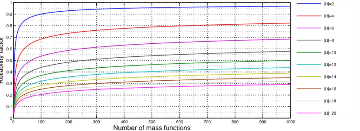
α_ki_i = f (| Ω |, | Cli_ki |) (25) The bigger| Ω | is, the more mass functions are needed to have a reliable cluster independence estimation. For example, if| Ω |= 5 then there are 25_{possible focal} elements, also independence estimation of a cluster containing 20 objects cannot be precise. No existing method to define such function f . Hence, we use simple heuristics as follows: α_ki_i = 1 − 1 | Cli ki | 1 |Ω| (26) As shown in figure 2, if| Ω | and number of mass functions in a cluster are big enough, cluster independence mass function is almost not discounted. Reliability factor is an increasing function of| Ω | and | Cli

ki | which favors big clusters

3_.

0 100 200 300 400 500 600 700 800 900 1000 0 0.1 0.2 0.3 0.4 0.5 0.6 0.7 0.8 0.9 1

Number of mass functions

Reliability factor |Ω|=2 |Ω|=4 |Ω|=6 |Ω|=8 |Ω|=10 |Ω|=12 |Ω|=14 |Ω|=16 |Ω|=18 |Ω|=20

Figure 2: Reliability factorsαi ki

4.4. Sources independence

Obtained mass functions quantify each matched clusters independence accord-ing to each source. Therefore, K mass functions are obtained for each source such that each mass function quantifies the independence of each couple of matched clusters. The combination of K mass functions for each source using the mean, defined by equation (12), is a mass function mΩI _{defining the whole independence}

of one source on another one:

mΩI,si_{(A) =} 1 K K

∑

With kj is the cluster matched to ki according to si. Two different mass

func-tions mΩI,s1 _{and m}ΩI,s2 _{are obtained for s}

1 and s2respectively. We note that mΩI,s1 is the combination of K mass functions representing the independence of matched clusters according to s1 defined using equation (24). Mass functions mΩI,s1 _and

mΩI,s2_{are different since cluster matchings are different which verifies the axiom of}

non-symmetry. β1

k1k2,β

2

k2k1 ∈ [0, 1] verify the non-negativity and the normalization

order to decide about sources independence Idsuch that:    Id(s1,s2) = BetP(Ind) Id(s1,s2) = BetP(Dep) (28)

If Id(s1,s2) > Id(s1,s2) we claim that sources s1 and s2are independent otherwise they are dependent.

4.5. General case

The method detailed above estimates the independence of one source on an-other one. Independence measure is non-symmetric because if a source s1is inde-pendent on a source s2then s2is not necessarily independent on s1and even if it is the case, degrees of independence are not necessarily the same.

It is wise to choose the minimum independence from Id(s1,s2) and Id(s2,s1) as the overall independence. Consequently, if at least one of two sources is dependent on the other, then sources are considered dependent. In other words, two sources are independent only if they are mutually independent. Hence, overall indepen-dence that is denoted I(s1,s2) is given by:

I(s1,s2) = min(Id(s1,s2), Id(s2,s1)) (29) We note that I(s1,s2) is non-negative, normalized, symmetric and identical. We define an independence measure, noted I, generalizing the independence for more than two sources verifying the following axioms:

1. Non-negativity: Many sources independence {s1,s2,s3, . . . ,sns}, noted Id(s1,s2, . . . ,sns) cannot be negative, it is either positive or null.

2. Normalization: Sources independence I is a degree in[0, 1]. The minimum 0 is reached when sources are completely dependent and the maximum 1 is reached when they are completely independent.

3. Symmetry: I(s1,s2,s3, . . . ,sns) is the sources’ overall independence and I(s1,s2,s3, . . . ,sns) = I(s2,s1,s3, . . . ,sns) = I(s3,s1,s2, . . . ,sns).

4. Identity: I(s1,s1,s1) = 0. It is obvious that any source is completely depen-dent on itself.

5. Increasing with inclusion: I(s1,s2) ≤ I(s1,s2,s3), more there are sources, more they are likely to be independent.

To compute the overall independence of ns sources{s1,s2, . . . ,sns},

indepen-dencies of pairs of sources are computed and the maximum4 independence is the sources overall independence:

I(s1,s2, . . . ,sns) = max(I(si,sj)), ∀i ∈ [1, ns] , j ∈]i, ns] (30)

or equivalently:

I(s1,s2, . . . ,sns) = max(min(Id(si,sj), Id(sj,si))), ∀i, j ∈ [1, ns] i 6= j (31)

Independence degree of sources is then integrated in the combination step using the following mixed combination rule.

5. Combination rule

Combination rules using conjunctive and/or disjunctive rules such as [2, 5, 6, 7, 8] are used when sources are completely independent but cautious and bold rules [10] tolerate redundant information and consequently can be used to combine mass functions which sources are dependent. In the combination step, sources de-pendence or indede-pendence hypothesis is intuitively made without any possibility of check. Sources independence degree is neither 0 nor 1 but a level over[0, 1].

The main question is “which combination rule to use when combining partially independent\dependent mass functions?”

In this paper, we propose a new mixed combination rule using conjunctive and cautious rules detailed in equations (8) and (13). In the case of totally dependent sources (where independence is 0), the cautious and proposed mixed combination rules are similar; whereas in the case of totally independent sources (independence is 1), the conjunctive and proposed combination rules are similar. In the case of an independence degree in]0, 1[, combined mass function is the average of conjunc-tive and cautious combinations weighted by sources’ independence degree.

Assume that two sources s1 and s2are independent with a degree γ such that γ = I(s1,s2); m1and m2 are mass functions provided by s1 and s2. The proposed mixed combination rule is defined as follows:

mMixed(A) = γ ∗ m ∩(A) + (1 − γ) ∗ m ∧(A), ∀A ⊆ Ω (32)

The degree of independence of a set of sources is given by equation (30), and the mixed combination of a set of mass functions {m1,m2, . . . ,mns} provided by

sources{s1,s2, . . . ,sns} is also a weighted average such that:

γ = I(s1,s2, . . . ,sns) (33)

Properties of the proposed mixed combination rule:

• Commutativity: Conjunctive and cautious rules are commutative. Indepen-dence measure is symmetric because sources’ degree of indepenIndepen-dence is the same for a set of sources. Then the proposed rule is commutative.

• Associativity: Conjunctive and cautious rule are associative but the proposed rule is not because independence degree of n sources and n+ 1 ones is not necessarily the same.

• Idempotent: Degree of independence of one source to itself is 0, in that case the proposed rule is equivalent to the cautious rule. As the cautious rule is idempotent, it is the case of the proposed mixed rule.

• Neutral element: Mixed combination rule does not have any neutral element. • Absorbing element: No absorbing element also.

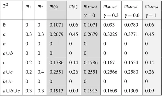
Example. Assume a frame of discernmentΩ = {a, b, c} and two sources s1and s2

providing two mass functions m1and m2. Table 1 illustrates conjunctive and cau-tious combinations as well as mixed combination in the cases whereγ = 0, γ = 0.3, γ = 0.6 and γ = 1. When γ = 0, mixed and cautious combinations are equivalent; whenγ = 1, mixed and conjunctive combinations are equivalent, otherwise it is a weighted average byγ ∈]0, 1[.

Finally, to illustrate the proposed mixed combination rule and compare it to other combination rules, three mass functions are generated randomly using algo-rithm 2. These mass functions are combined with conjunctive, Dempster, Yager, disjunctive, cautious and mean combination rules. They are also combined with the mixed combination rule with different independence levels.

Figure 3 illustrates distances5 between the mixed combination with several de-grees of independence and combined mass functions using conjunctive, Dempster, Yager, disjunctive, cautious and mean combination rules. Distances between mixed combination with several independence degrees; and Yager, disjunctive, mean and Dempster’s rules are linear and decreasing proportionally toγ.

Table 1: Combination of two mass functions

2Ω m1 m2 m ∧ m ∩ mMixed mMixed mMixed mMixed

γ = 0 γ = 0.3 γ = 0.6 γ = 1 /0 0 0 0.1071 0.06 0.1071 0.093 0.0789 0.06 a 0.3 0.3 0.2679 0.45 0.2679 0.3225 0.3771 0.45 b 0 0 0 0 0 0 0 0 a∪ b 0 0 0 0 0 0 0 0 c 0.2 0 0.1786 0.14 0.1786 0.167 0.1554 0.14 a∪ c 0.2 0.4 0.2551 0.26 0.2551 0.2566 0.2580 0.26 b∪ c 0 0 0 0 0 0 0 0 a∪ b ∪ c 0.3 0.3 0.1913 0.09 0.1913 0.1609 0.1305 0.09 6. Experiments

Because of the lack of real evidential data, we use generated mass functions to test the method detailed above. Moreover, it is difficult to simulate all situations with all possible combinations of focal elements for several degrees of indepen-dence between sources. First, we generate two sets of mass functions for two sources s1and s2; then we illustrate for three sources.

6.1. Generated data depiction

Generating sets of n mass functions for several sources depends on sources independence. We discern cases of independent and dependent sources.

6.1.1. Independent sources

In general, to generate mass functions some information are needed: the num-ber of hypotheses in the frame of discernment,| Ω | and the number of mass

func-0 0.1 0.2 0.3 0.4 0.5 0.6 0.7 0.8 0.9 1 0 0.1 0.2 0.3 0.4 0.5 0.6 0.7 0.8 0.9 1 Independence degrees Distances

Distances to the Conjunctive combination Distances to Dempster combination Distances to Yager combination Distances to the Disjunctive combination Distances to the Cautious combination Distances to the Mean combination

Figure 3: Distances between combined mass functions

tions. We note that number of focal elements, and masses are chosen randomly. In the case of independent sources, masses can be anywhere and focal elements of both sources are chosen independently. Mass functions of s1and s2are generated following algorithm 2. We note that focal elements, their number and BBMs are chosen randomly according to the universal low.

Algorithm 2 Independent mass functions generating Require: |Ω|, n : number of mass functions

1: for i= 1 to n do

2: Choose randomly| F |, the number of focal elements on [1, |2Ω_|].

3: Choose randomly| F | focal elements noted F.

4: Divvy the interval[0, 1] into |F| continuous sub-intervals.

5: Focal elementsBBMs are intervals sizes.

6: end for

7: return n mass functions

6.1.2. Dependent sources

The case of dependent sources is a bit difficult to simulate as several scenarios can occur. In this section, we will try to illustrate the most common situations.

Generated mass functions for dependent sources are supposed to be consistent and do not enclose any internal conflict [27]. Consistent mass functions contain at least one focal element common to all focal sets. Figure 4 illustrates a consistent mass function where all focal elements{A, B, C, D} intersect.

Figure 4: Consistent belief function

Algorithm 3 generates a set of n consistent mass functions6defined on a frame of discernment of size| Ω |. In the case of dependent sources, they are almost consistent and at least one of them is dependent on the other. To simulate the case where one source is dependent on another one, consistent mass functions of the first one are generated following algorithm 3, then those of the second source are generated knowing decisions of the first one. Algorithm 4 generates a set of mass functions that are dependent on another set of mass functions. Dependence is due to the knowledge of other source’s decisions.

6.2. Results of tests

Algorithms detailed in the previous section are used to test some cases of sources’ dependence and independence. We note that in extreme cases where mass functions are certain or even when focal elements do not intersect; maximal values of independence are obtained. In the case of perfect dependence; mass functions

Algorithm 3 Consistent mass functions generating Require: |Ω|, n : number of mass functions

1: for i= 1 to n do

2: Choose randomly a focal setωi(it can be a single point) fromΩ.

3: Find the set S of all focal sets includingωi.

4: Choose randomly| F |, the number of focal elements on [1, |S|].

5: Choose randomly| F | focal elements from S noted F.

6: Divvy the interval[0, 1] into |F| continuous sub-intervals.

7: BBMs of focal elements are intervals sizes.

8: end for

9: return n consistent mass functions

have the same focal elements; however, clusters contain mass functions with con-sistent focal elements. Clustering is performed according to focal elements and clusters are perfectly linked.

6.2.1. Independent sources

In this paragraph, mass functions are independent. Focal elements andBBMs are randomly chosen ensuing algorithm 2. For tests, we choose| Ω |= 5 which is considered as medium-sized frame of discernment and n= 100. Table 2 illustrates the mean of 100 tests in the case of independent sources. The mean of 100 tests for two dependent sources yields to a degree of independence γ = 0.68, thus sources are independent. Assume that m1 and m2, given in table 1, are provided by two sources s1and s2which independence degree is given in table 2. Combination of

m1and m2is given in table 3.

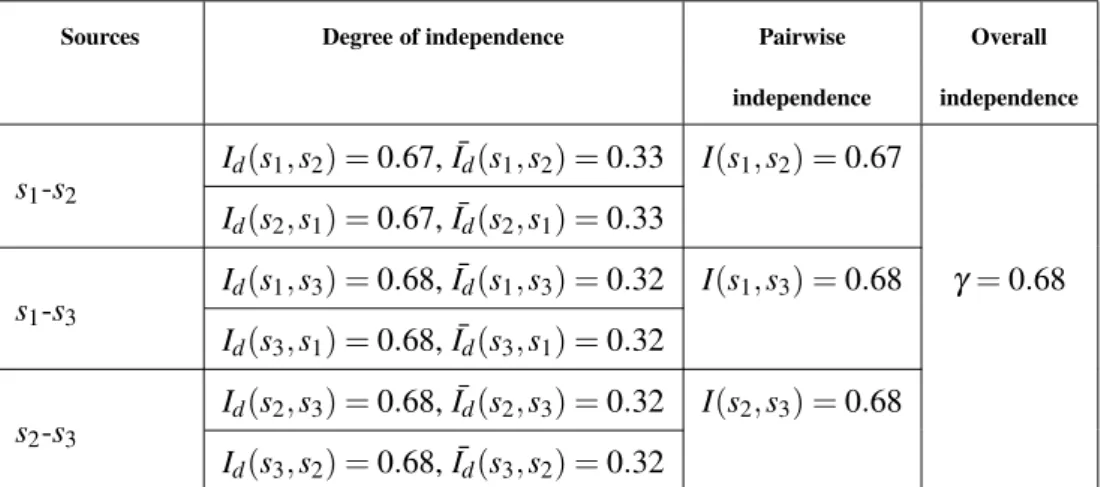
To illustrate the case of three independent sources, three sets of 100 indepen-dent mass functions are generated following algorithm 2 with| Ω |= 5. The mean of 100 tests are illustrated in table 4.

Algorithm 4 Dependent mass functions generating

Require: |Ω|, n : number of mass functions, d decision of another source

1: for i= 1 to n do

2: Find the set S of all focal sets including d.

3: Choose randomly| F |, the number of focal elements on [1, |S|].

4: Choose randomly| F | focal elements from S noted F.

5: Divvy the interval[0, 1] into |F| continuous sub-intervals.

6: Focal elementsBBMs are intervals sizes.

7: end for

8: return n consistent mass functions

Table 2: Mean of 100 tests on 100 generated mass functions for two sources

Dependence type Degree of independence Overall independence

Independence Id(s1 ,s2) = 0.68, ¯Id(s1,s2) = 0.32 γ = 0.68 Id(s2,s1) = 0.68, ¯Id(s2,s1) = 0.32 Dependence Id(s1,s2) = 0.34, ¯Id(s1,s2) = 0.66 γ = 0.34 Id(s2,s1) = 0.35, ¯Id(s2,s1) = 0.65 6.2.2. Dependent sources

In the case of dependent sources, mass functions are generated ensuing algo-rithms 3 and 4. For tests, we choose| Ω |= 5 and n = 100. We generate 100 mass functions of both s1and s2for 100 times and then compute the average of Id(s1,s2), Id(s2,s1) and I(s1,s2). Table 2 illustrates the mean of 100 independence degrees of two dependent sources providing each one 100 randomly generated mass func-tions. These sources are dependent with a degree 1− γ = 0.66. In table 3, m1and

m2are combined using the mixed rule whenγ = 0.34.

Table 3: Mixed combination of m1and m2 2Ω m1 m2 mMixed mMixed γ = 0.68 γ = 0.34 /0 0 0 0.092 0.076 a 0.3 0.3 0.3262 0.3881 b 0 0 0 0 a∪ b 0 0 0 0 c 0.2 0 0.1662 0.1531 a∪ c 0.2 0.4 0.2567 0.2583 b∪ c 0 0 0 0 a∪ b ∪ c 0.3 0.3 0.1589 0.1244

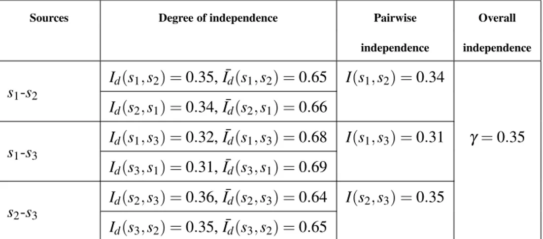
functions are generated following algorithms 3 and 4 when| Ω |= 5. The mean of 100 degrees of independence are illustrated in table 5.

Finally, assume that m1, m2and m3of table 6 are three mass functions defined on a frame of discernmentΩ = {a, b, c} and provided by three dependent sources. The mixed combined mass function when their degree of independence isγ = 0.35 is also given in table 6.

7. Conclusion

In this paper, we proposed a method to learn sources cognitive independence in order to use the appropriate combination rule either when sources are cognitively dependent or independent. Sources are cognitively independent if they are differ-ent; not communicating and they have distinct evidential corpora. The proposed statistical approach is based on a clustering algorithm applied to mass functions

Table 4: Mean of 100 tests on 100 generated mass functions for three independent sources

Sources Degree of independence Pairwise Overall

independence independence s1-s2 Id(s1,s2) = 0.67, ¯Id(s1,s2) = 0.33 I(s1,s2) = 0.67 Id(s2,s1) = 0.67, ¯Id(s2,s1) = 0.33 s1-s3 Id(s1,s3) = 0.68, ¯Id(s1,s3) = 0.32 I(s1,s3) = 0.68 γ = 0.68 Id(s3,s1) = 0.68, ¯Id(s3,s1) = 0.32 s2-s3 Id(s2,s3) = 0.68, ¯Id(s2,s3) = 0.32 I(s2,s3) = 0.68 Id(s3,s2) = 0.68, ¯Id(s3,s2) = 0.32

provided by several sources. A pair of sources independence is deduced from weights of linked clusters after a matching of their clusters. Independence degree of sources can either guide the choice of the combination rule if it is either 1 or 0; when it is a degree over]0, 1[, we propose a new combination rule that weights the conjunctive and cautious combinations with sources’ independence degree.

References

[1] L. A. Zadeh, Fuzzy sets, Information and Control 8 (3) (1965) 338–353. [2] D. Dubois, H. Prade, Representation and combination of uncertainty with

belief functions and possibility measures, Computational Intelligence 4 (3) (1988) 244–264.

[3] A. P. Dempster, Upper and lower probabilities induced by a multivalued map-ping, The Annals of Mathematical Statistics 38 (2) (1967) 325–339.

Table 5: Mean of 100 tests on 100 generated mass functions for three dependent sources

Sources Degree of independence Pairwise Overall

independence independence s1-s2 Id(s1,s2) = 0.35, ¯Id(s1,s2) = 0.65 I(s1,s2) = 0.34 Id(s2,s1) = 0.34, ¯Id(s2,s1) = 0.66 s1-s3 Id(s1,s3) = 0.32, ¯Id(s1,s3) = 0.68 I(s1,s3) = 0.31 γ = 0.35 Id(s3,s1) = 0.31, ¯Id(s3,s1) = 0.69 s2-s3 Id(s2,s3) = 0.36, ¯Id(s2,s3) = 0.64 I(s2,s3) = 0.35 Id(s3,s2) = 0.35, ¯Id(s3,s2) = 0.65

[4] G. Shafer, A mathematical theory of evidence, Princeton University Press, 1976.

[5] A. Martin, C. Osswald, Toward a combination rule to deal with partial con-flict and specificity in belief functions theory, in: International Conference on Information Fusion, Qu´ebec, Canada, 2007, pp. 1–8.

[6] C. K. Murphy, Combining belief functions when evidence conflicts, Decision Support Systems 29 (1) (2000) 1–9.

[7] P. Smets, R. Kennes, The transferable belief model, Artificial Intelligence 66 (2) (1994) 191–234.

[8] R. R. Yager, On the Dempster-Shafer framework and new combination rules, Information Sciences 41 (2) (1987) 93–137.

[9] E. Lef`evre, Z. Elouedi, How to preserve the conflict as an alarm in the com-bination of belief functions?, Decision Support Systems 56 (2013) 326–333.

Table 6: Mixed combination of m1, m2and m3 2Ω m1 m2 m3 mMixed γ = 0.35 /0 0 0 0 0 a 0 0 0 0 b 0 0 0 0 a∪ b 0 0 0 0 c 0.03 0.05 0 0.32 a∪ c 0.39 0.07 0.04 0.24 b∪ c 0.3 0.47 0.22 0.29 a∪ b ∪ c 0.28 0.41 0.74 0.15

[10] T. Denœux, Conjunctive and disjunctive combination of belief functions in-duced by nondistinct bodies of evidence, Artificial Intelligence 172 (2-3) (2008) 234–264.

[11] B. Ben Yaghlane, P. Smets, K. Mellouli, Belief function independence: I. The marginal case, International Journal of Approximate Reasoning 29 (1) (2002) 47–70.

[12] B. Ben Yaghlane, P. Smets, K. Mellouli, Belief function independence: II. The conditional case, International Journal of Approximate Reasoning 31 (1-2) (200(1-2) 31–75.

[13] P. Smets, Belief functions: The disjunctive rule of combination and the gen-eralized Bayesian theorem, International Journal of Approximate Reasoning 9 (1) (1993) 1–35.

[14] P. Smets, The combination of evidence in the transferable belief model, IEEE Transactions on Pattern Analysis and Machine Intelligence 12 (5) (1990) 447–458.

[15] P. Smets, The canonical decomposition of a weighted belief, in: Interna-tional Joint Conference on Artificial Intelligence, Vol. 2, Morgan Kaufman, Montr´eal, Qu´ebec, Canada, 1995, pp. 1896–1901.

[16] L. A. Zadeh, A mathematical theory of evidence (book review), AI magazine 5 (3) (1984) 81–83.

[17] P. Smets, The nature of the unnormalized beliefs encountered in the transfer-able belief model, in: D. Dubois, M. P. Wellman (Eds.), International confer-ence on Uncertainty in Artificial Intelligconfer-ence, Morgan Kaufmann, Stanford, California, USA, 1992, pp. 292–297.

[18] A. Martin, A.-L. Jousselme, C. Osswald, Conflict measure for the discounting operation on belief functions, in: International Conference on Information Fusion, Cologne, Germany, 2008, pp. 1–8.

[19] A.-L. Jousselme, D. Grenier, E. Boss´e, A new distance between two bodies of evidence, Information Fusion 2 (2) (2001) 91–101.

[20] S. Ben Hariz, Z. Elouedi, K. Mellouli, Clustering approach using belief func-tion theory, in: J. Euzenat, J. Domingue (Eds.), 7th Conference of the Euro-pean Society for Fuzzy Logic and Technology, Vol. 4183 of Lecture Notes in Computer Science, Atlantis Press, Varna, Bulgaria, 2006, pp. 162–171. [21] M. Chebbah, A. Martin, B. Ben Yaghlane, About sources dependence in the

theory of belief functions, in: T. Denœux, M.-H. Masson (Eds.), International Conference on Belief Functions, Vol. 164 of Advances in Intelligent and Soft

Computing, Springer Berlin Heidelberg, Compi`egne, France, 2012, pp. 239– 246.

[22] P. Smets, R. Kruse, Uncertainty Management in Information Systems: From Needs to Solutions, Springer US, Boston, 1997, Ch. The Transferable Belief Model for Belief Representation, pp. 343–368.

[23] J. Munkres, Algorithms for the Assignment and Transportation Problems, Journal of the Society for Industrial and Applied Mathematics 5 (1) (1957) 32–38.

[24] F. Bourgeois, J.-C. Lassalle, An Extension of the Munkers Algorithm for the Assignement Problem to Rectangular Matrices, Communication of the ACM 12 (14) (1971) 802–804.

[25] C. Wemmert, P. Ganc¸arski, A multi-view voting method to combine unsu-pervised classifications, in: IASTED International Conference on Artificial Intelligence and Applications, M´alaga, Spain, 2002, pp. 447–453.

[26] P. Ganc¸arski, C. Wemmert, Collaborative multi-strategy classification: Ap-plication to per-pixel analysis of images, in: International Workshop on Mul-timedia Data Mining: Mining Integrated Media and Complex Data, Chicago, Illinois, USA, 2005, pp. 15–22.

[27] M. Daniel, Conflicts within and between belief functions, in: IPMU, 2010, pp. 696–705.