ScienceDirect
Available online at www.sciencedirect.com
Transportation Research Procedia 25 (2017) 2566–2573
2352-1465 © 2017 The Authors. Published by Elsevier B.V.
Peer-review under responsibility of WORLD CONFERENCE ON TRANSPORT RESEARCH SOCIETY. 10.1016/j.trpro.2017.05.301
www.elsevier.com/locate/procedia
10.1016/j.trpro.2017.05.301
© 2017 The Authors. Published by Elsevier B.V.
Peer-review under responsibility of WORLD CONFERENCE ON TRANSPORT RESEARCH SOCIETY.
2352-1465 Available online at www.sciencedirect.com
ScienceDirect
Transportation Research Procedia 00 (2017) 000–000
www.elsevier.com/locate/procedia
2214-241X © 2017 The Authors. Published by Elsevier B.V.
Peer-review under responsibility of WORLD CONFERENCE ON TRANSPORT RESEARCH SOCIETY.
World Conference on Transport Research - WCTR 2016 Shanghai. 10-15 July 2016
A bi-level Random Forest based approach for estimating O-D
matrices: Preliminary results from the Belgium National Household
Travel Survey
Ismaïl Saadi
a, Ahmed Mustafa
a, Jacques Teller
a, Mario Cools
a,*aUniversity of Liège, ARGENCO, LEMA, Allée de la Découverte 9, Quartier Polytech 1, 4000 Liège, Belgium
Abstract
This paper presents a random forests (RF) based approach to estimate an origin-destination (O-D) matrix on the basis of a travel survey. The trips are predicted on a weekly basis to retain a maximum number of recorded trips for model calibration and validation. The flexibility of the procedure ensures an extension for further disaggregate estimates of O-D matrices. We adopt data stemming from the Belgium National Household Travel Survey as an input for estimating the O-D matrix, in contrast to conventional approaches that exploit traffic counts. Regarding the methodology, preliminary results indicate that the RF approach provides interesting approximations of the O-D traffic flows. The mix of “bagging” and “random subspace” principles included in the RF framework confines the risk of overfitting. Furthermore, the approach is capable of handling large dataset in terms of the number of features and the number of observations.
© 2017 The Authors. Published by Elsevier B.V.
Peer-review under responsibility of WORLD CONFERENCE ON TRANSPORT RESEARCH SOCIETY.
Keywords: O-D matrix estimation; Random Forest; Travel Survey; Bagging; Random Subspace.
1. Background
From a methodological point of view, the estimation of travel demand forecasts led to the development of variety of approaches to predict origin-destination matrices. Because of the significant required time and cost, O-D matrices are generally estimated indirectly through traffic measurements (Talebian and Shafahi, 2015).
* Corresponding author. Tel.: +32 4 366 48 13; fax: +32 4 366 95 62.
E-mail address: mario.cools@ulg.ac.be.
Available online at www.sciencedirect.com
ScienceDirect
Transportation Research Procedia 00 (2017) 000–000
www.elsevier.com/locate/procedia
2214-241X © 2017 The Authors. Published by Elsevier B.V.
Peer-review under responsibility of WORLD CONFERENCE ON TRANSPORT RESEARCH SOCIETY.
World Conference on Transport Research - WCTR 2016 Shanghai. 10-15 July 2016
A bi-level Random Forest based approach for estimating O-D
matrices: Preliminary results from the Belgium National Household
Travel Survey
Ismaïl Saadi
a, Ahmed Mustafa
a, Jacques Teller
a, Mario Cools
a,*aUniversity of Liège, ARGENCO, LEMA, Allée de la Découverte 9, Quartier Polytech 1, 4000 Liège, Belgium
Abstract
This paper presents a random forests (RF) based approach to estimate an origin-destination (O-D) matrix on the basis of a travel survey. The trips are predicted on a weekly basis to retain a maximum number of recorded trips for model calibration and validation. The flexibility of the procedure ensures an extension for further disaggregate estimates of O-D matrices. We adopt data stemming from the Belgium National Household Travel Survey as an input for estimating the O-D matrix, in contrast to conventional approaches that exploit traffic counts. Regarding the methodology, preliminary results indicate that the RF approach provides interesting approximations of the O-D traffic flows. The mix of “bagging” and “random subspace” principles included in the RF framework confines the risk of overfitting. Furthermore, the approach is capable of handling large dataset in terms of the number of features and the number of observations.
© 2017 The Authors. Published by Elsevier B.V.
Peer-review under responsibility of WORLD CONFERENCE ON TRANSPORT RESEARCH SOCIETY.
Keywords: O-D matrix estimation; Random Forest; Travel Survey; Bagging; Random Subspace.
1. Background
From a methodological point of view, the estimation of travel demand forecasts led to the development of variety of approaches to predict origin-destination matrices. Because of the significant required time and cost, O-D matrices are generally estimated indirectly through traffic measurements (Talebian and Shafahi, 2015).
* Corresponding author. Tel.: +32 4 366 48 13; fax: +32 4 366 95 62.
E-mail address: mario.cools@ulg.ac.be.
2 I. Saadi et al. / Transportation Research Procedia 00 (2017) 000–000
In general, prior estimates of OD matrices and aggregate traffic counts (or speed measures) are used as a starting point for estimating O-D matrices (Bera and Rao, 2011; Frederix et al., 2013). It is assumed that traffic counts are widely available at a moderate cost. The nature (static or dynamic) of the O-D matrices depends on the specificities of the employed traffic assignment method.
From a methodological perspective, various techniques have been proposed for estimating and/or correcting O-D matrices using traffic counts. Under the assumption of a static O-D matrix, the maximum likelihood (Bell, 1983; Maher, 1983) and the Generalized least squares (Cascetta, 1984) approaches have been used to provide estimations by maximizing the probability to observe an estimated O-D matrix resulting in the observed traffic counts.To meet the needs of real-time traffic management and given the improvements with regard to dynamic traffic assignment methods, a shift from static towards dynamic O-D matrices was inevitable. In this regard, Ashok and Ben-Akiva (2002) outlined the importance of considering the dynamic nature of traffic demand. Thus, different studies proposed estimations of O-D matrices using dynamic traffic assignment methods (Flötteröd et al., 2011). Lorenzo and Matteo (2013) also started from traffic measurements of road segments to find an approximation of the O-D matrix. It their study, neural networks are used to forecast the relationship between traffic flows and O-D pairs. For selecting the most relevant variables, they perform a Principal Component Analysis (PCA). Toledo and Kolechkina (2013) presented linear approximations of the assignment matrix using traffic counts related to specific road segments and other past demand information. For congested networks, Frederix et al. (2014) estimated dynamic O-D matrices using a hierarchical decomposition scheme. The main idea consists in distinguishing the congested subareas for estimating more accurate O-D matrices. Besides, Djukic et al. (2014) introduced a new formulation based on Kalman filter where they demonstrate an effective quality improvement of the O-D matrix estimation. In addition, Perrakis et al. (2012) proved that good estimates of O-D flows can be derived from historical data (e.g. census) by applying Bayesian statistics. Validation tests of their model suggested good predictive results (Perrakis et al., 2015).
Regarding the reliability of travel surveys to find correct OD estimates, Stopher and Greaves (2007) underlined that travel surveys may contain mistakes regarding non-response, limited sample size, under-representation of trips and errors in travel time measurements. As a consequence, the shift towards other data such as traffic counts appeared to be an alternative to overcome potential errors induced by travel surveys.
In this paper, we present a substantially different approach with respect to the classic O-D matrix estimation procedure, from both data and methodological perspectives. Regarding data perspectives, instead of using traffic counts, we propose a method that estimates O-D flows from disaggregated travel diary data. Although traffic counts might be readily available in some countries, in the case of Belgium, such data are difficult to obtain because of institutional issues and the absence of a large covering structure allowing the recording of such data. In this context, there is a clear need to use alternative data (e.g. micro-samples) to address this problem. Furthermore, a disaggregate estimation of O-D flows is necessary for favoring reliable and efficient demand models where traffic counts could ideally be used as validation dataset (Marzano et al., 2009). In addition, the use of traffic counts for calibrating O-D traffic flows can lead to a risk of overfitting, thereby preventing an important source of observed measures for validation purposes. Besides, traffic counts are also frequently used for O-D traffic flows corrections enabling further approximations within the model system (Marzano et al., 2009).
Regarding methodological perspectives, the total variance present in travel diary data is mitigated by using a Random Forests (RF) based approach. As mentioned by Cools et al. (2010), errors emanating from the sampling variance represent an important portion of the variance. In this context, we propose a RF algorithm because of its property in mitigating the variance through “bagging” procedure and “random sub-space” principles.
2. Data
In this paper, we use travel diary data stemming from the 2010 Belgium National Household Travel Survey for model calibration. This survey contains a detailed dataset describing the daily trips of the Belgian citizens. An adequate preparation of the data is important before running any simulation. We first identify the most relevant explanatory variables present in the dataset. In this regard, we have selected individuals’ age, gender and socio-professional status. With respect to modal choice, individuals' usage frequency of eight different modes is considered. Furthermore, we have also included transport title and driving license ownership as predictors.
Ismaïl Saadi et al. / Transportation Research Procedia 25 (2017) 2566–2573 2567
ScienceDirect
Transportation Research Procedia 00 (2017) 000–000
www.elsevier.com/locate/procedia
2214-241X © 2017 The Authors. Published by Elsevier B.V.
Peer-review under responsibility of WORLD CONFERENCE ON TRANSPORT RESEARCH SOCIETY.
World Conference on Transport Research - WCTR 2016 Shanghai. 10-15 July 2016
A bi-level Random Forest based approach for estimating O-D
matrices: Preliminary results from the Belgium National Household
Travel Survey
Ismaïl Saadi
a, Ahmed Mustafa
a, Jacques Teller
a, Mario Cools
a,*aUniversity of Liège, ARGENCO, LEMA, Allée de la Découverte 9, Quartier Polytech 1, 4000 Liège, Belgium
Abstract
This paper presents a random forests (RF) based approach to estimate an origin-destination (O-D) matrix on the basis of a travel survey. The trips are predicted on a weekly basis to retain a maximum number of recorded trips for model calibration and validation. The flexibility of the procedure ensures an extension for further disaggregate estimates of O-D matrices. We adopt data stemming from the Belgium National Household Travel Survey as an input for estimating the O-D matrix, in contrast to conventional approaches that exploit traffic counts. Regarding the methodology, preliminary results indicate that the RF approach provides interesting approximations of the O-D traffic flows. The mix of “bagging” and “random subspace” principles included in the RF framework confines the risk of overfitting. Furthermore, the approach is capable of handling large dataset in terms of the number of features and the number of observations.
© 2017 The Authors. Published by Elsevier B.V.
Peer-review under responsibility of WORLD CONFERENCE ON TRANSPORT RESEARCH SOCIETY.
Keywords: O-D matrix estimation; Random Forest; Travel Survey; Bagging; Random Subspace.
1. Background
From a methodological point of view, the estimation of travel demand forecasts led to the development of variety of approaches to predict origin-destination matrices. Because of the significant required time and cost, O-D matrices are generally estimated indirectly through traffic measurements (Talebian and Shafahi, 2015).
* Corresponding author. Tel.: +32 4 366 48 13; fax: +32 4 366 95 62.
E-mail address: mario.cools@ulg.ac.be.
2 I. Saadi et al. / Transportation Research Procedia 00 (2017) 000–000
In general, prior estimates of OD matrices and aggregate traffic counts (or speed measures) are used as a starting point for estimating O-D matrices (Bera and Rao, 2011; Frederix et al., 2013). It is assumed that traffic counts are widely available at a moderate cost. The nature (static or dynamic) of the O-D matrices depends on the specificities of the employed traffic assignment method.
From a methodological perspective, various techniques have been proposed for estimating and/or correcting O-D matrices using traffic counts. Under the assumption of a static O-D matrix, the maximum likelihood (Bell, 1983; Maher, 1983) and the Generalized least squares (Cascetta, 1984) approaches have been used to provide estimations by maximizing the probability to observe an estimated O-D matrix resulting in the observed traffic counts.To meet the needs of real-time traffic management and given the improvements with regard to dynamic traffic assignment methods, a shift from static towards dynamic O-D matrices was inevitable. In this regard, Ashok and Ben-Akiva (2002) outlined the importance of considering the dynamic nature of traffic demand. Thus, different studies proposed estimations of O-D matrices using dynamic traffic assignment methods (Flötteröd et al., 2011). Lorenzo and Matteo (2013) also started from traffic measurements of road segments to find an approximation of the O-D matrix. It their study, neural networks are used to forecast the relationship between traffic flows and O-D pairs. For selecting the most relevant variables, they perform a Principal Component Analysis (PCA). Toledo and Kolechkina (2013) presented linear approximations of the assignment matrix using traffic counts related to specific road segments and other past demand information. For congested networks, Frederix et al. (2014) estimated dynamic O-D matrices using a hierarchical decomposition scheme. The main idea consists in distinguishing the congested subareas for estimating more accurate O-D matrices. Besides, Djukic et al. (2014) introduced a new formulation based on Kalman filter where they demonstrate an effective quality improvement of the O-D matrix estimation. In addition, Perrakis et al. (2012) proved that good estimates of O-D flows can be derived from historical data (e.g. census) by applying Bayesian statistics. Validation tests of their model suggested good predictive results (Perrakis et al., 2015).
Regarding the reliability of travel surveys to find correct OD estimates, Stopher and Greaves (2007) underlined that travel surveys may contain mistakes regarding non-response, limited sample size, under-representation of trips and errors in travel time measurements. As a consequence, the shift towards other data such as traffic counts appeared to be an alternative to overcome potential errors induced by travel surveys.
In this paper, we present a substantially different approach with respect to the classic O-D matrix estimation procedure, from both data and methodological perspectives. Regarding data perspectives, instead of using traffic counts, we propose a method that estimates O-D flows from disaggregated travel diary data. Although traffic counts might be readily available in some countries, in the case of Belgium, such data are difficult to obtain because of institutional issues and the absence of a large covering structure allowing the recording of such data. In this context, there is a clear need to use alternative data (e.g. micro-samples) to address this problem. Furthermore, a disaggregate estimation of O-D flows is necessary for favoring reliable and efficient demand models where traffic counts could ideally be used as validation dataset (Marzano et al., 2009). In addition, the use of traffic counts for calibrating O-D traffic flows can lead to a risk of overfitting, thereby preventing an important source of observed measures for validation purposes. Besides, traffic counts are also frequently used for O-D traffic flows corrections enabling further approximations within the model system (Marzano et al., 2009).
Regarding methodological perspectives, the total variance present in travel diary data is mitigated by using a Random Forests (RF) based approach. As mentioned by Cools et al. (2010), errors emanating from the sampling variance represent an important portion of the variance. In this context, we propose a RF algorithm because of its property in mitigating the variance through “bagging” procedure and “random sub-space” principles.
2. Data
In this paper, we use travel diary data stemming from the 2010 Belgium National Household Travel Survey for model calibration. This survey contains a detailed dataset describing the daily trips of the Belgian citizens. An adequate preparation of the data is important before running any simulation. We first identify the most relevant explanatory variables present in the dataset. In this regard, we have selected individuals’ age, gender and socio-professional status. With respect to modal choice, individuals' usage frequency of eight different modes is considered. Furthermore, we have also included transport title and driving license ownership as predictors.
2568 Ismaïl Saadi et al. / Transportation Research Procedia 25 (2017) 2566–2573
I. Saadi et al. / Transportation Research Procedia 00 (2017) 000–000 3 Table 1. Characteristics of the selected features
Variables Descriptive statistics
Socio-demographics
Age Mean: 46.54, Std. Dev.: 21.08
Gender Male: 0.48, Female: 0.52
Socio-professional Status** 1: 0.08%, 2: 17.23%, 3: 4.3%, 4: 5.54%, 5: 28.14%, 6: 2.23%, 7: 7.72%, 8: 3.51%, 9: 21.72%, 10: 3.96%, 11: 1.11%, 12: 3.76%, 13: 0.23%, 14: 0.48% Transport-related characteristics* Foot 1: 40.37%, 2: 28.02%, 3: 13.80%, 4: 5.42%, 5: 12.39% Bicycle 1: 7.39%, 2: 11.76%, 3: 12.51%, 4: 18.29%, 5: 50.04% Motorcycle 1: 1.16%, 2: 1.25%, 3: 1.79%, 4: 2.35%, 5: 93.45% Public Transport 1: 15.42%, 2: 12.11%, 3: 11.87%, 4: 23.83%, 5: 36.77% Taxi 1: 0.77%, 2: 0.77%, 3: 2.64%, 4: 15.08%, 5: 80.74% Car as Driver 1: 39.34%, 2: 17.99%, 3: 4.47%, 4: 2.03%, 5: 36.18% Car as Passenger 1: 13.39%, 2: 28.63%, 3: 20.72%, 4: 14.64%, 5: 22.62% Plane 1: 0.27%, 2: 0.52%, 3: 1.44%, 4: 37.49%, 5: 60.29%
Transport title Yes: 83.90%, No: 16.10%
Driving license In progress: 4.90%, Yes: 24.87%, No: 70.23%
Worker Yes: 40.89%, No: 59.11%
Student Yes: 17.63%, No: 82.37%
Not worker, not student Yes: 41.67%, No: 58.33%
*1: at least five days/week, 2: 1 to few days/week, 3: 1 to few days/month, 4: 1 to few days/year, 5: never
**1: not schooled children, 2: student, 3: Housewife/Househusband, 4: Job-seeker, 5: Retired person, 6: Handicapped person, 7: Worker, 8: Executive, 9: Employee, 10: Self-employed worker, 11: Liberal profession, 12: Teacher, 13: Farmer, 14: Other
3. Methodology
As a continuation of the ensemble learning methods, Breiman (2001) developed random forests (RF) which consist in the combination of tree predictors. Particularly, RF are a coupling of those two techniques: the concept of bagging, introduced by Breiman (1996), and a set of randomly selected explanatory variables (features) for growing trees (Amit and Geman, 1997; Ho, 1995). The bagging (also called bootstrap aggregation) strategy is a technique where each individual tree-based model is trained on the basis of a bootstrap sample coming from the training dataset. The strength of RF resides in its capacity to mitigate the error as long as the number of trees is important. Thus, as outlined by Breiman (2001), the generalization of the error depends upon the quality of each decision tree as well their respective cross-correlation.
By introducing the concept of random selection of features, the modelling process results in an ensemble of decision trees, presenting more robustness with respect to noise. As a result, trees are allowed to be partially overfitted to their respective bootstrap. However, the overfitting phenomenon becomes trivial when the classifiers are assembled by averaging or other related tree bagger techniques. Random selection of features presents another characteristic distinguishing the decision trees enabling, in this regard, more diversification. Depending on the nature of the response (classification or regression), the number of random selected variables is respectively set at sqrt(n) and n/3. The random subspace strategy included in RF is very powerful as the diversity between the trees is increased by defining high numbers of bootstraps of the partial feature space. Considered separately from other bagging techniques, some studies have suggested that the Random Subspace method presents acceptable results when half of the total numbers of features are selected. Furthermore, for a larger dataset (with several features) a more important number of randomly selected features increases the performance of the methodology. On the contrary, a lower number of features combined with existing irrelevant features decreases the performance. In this context, RF allow insertion of bagging algorithms, thereby mitigating the negative effects of the random subspace methods (Sammut and Webb, 2011).
The final outcome of the RF model is a combination of the set of the different outputs provided by the set of classifiers. Averaging is used for estimating regression models, while majority voting is employed for classification trees. Three factors can explain the performances of RF; correlation between individual trees, the performance with
4 I. Saadi et al. / Transportation Research Procedia 00 (2017) 000–000
respect to each tree and the total number of trees. Hastie et al. (2009) defined the variance of RF by the following equation: 2 1 2 var(RF) T (1)
The variance of each individual tree is represented by σ2, ρ is the correlation between the trees and T is the
number of trees within the ensemble. The mitigation of the second term is possible through the increase of the total number of trees such that the term converges towards zero, thus one must ensure that T is relatively high. A low value of the correlation factor between any tree pair ρ is achieved by an efficient random selection of s features out of n (the total number of features). In this regard, we can also reduce the effects of the first term of the equation.
A strengthening of the performance of every tree of the ensemble will reduce their respective variance. Note that a decrease of ρ also comes along with a weakness of performances of every tree. Thus, with respect to this direct relation between ρ and σ2, it should be emphasized that finding a good compromise is important so that the global
equation of the variance is minimized.
In this paper, we build two predictive RF models to allow a bi-level estimation of the origin-destination matrix. First, a relevant set of explanatory variables are selected from the full reference dataset to predict the trip origin (response 1) at the local scale. Note that we split the dataset into training and validation sets. Consequently, a second model is calibrated for predicting the trip destinations. Given the fact that the trip destinations are also dependent on the trip origins, the latter will be considered as a predictor within the second model.
In a random forest, each classification tree is characterized by a certain number of randomly selected attributes to operate a split at the nodes and is trained with respect to a bootstrap. Thus, the classification tree k called SSk can be represented by the following expression:
1 1 1 1 2 2 2 2 a b s a b s k aN bN sN N
f
f
f
C
f
f
f
C
SS
f
f
f
C
(2)where k is the tree reference number; s is the number of randomly selected features out of the total number of features T; N is the number of observations of the sub-sample k. In this way, each decision tree is capable of predicting what should be the class for any input vector
v
in
( , ,..., )
f f
a bf
vFinally, in order to assemble all the outcomes, a majority vote is used for classification or an averaging of the outcomes in the case of a regression.
Table 1. Characteristics of the selected features
Variables Descriptive statistics
Socio-demographics
Age Mean: 46.54, Std. Dev.: 21.08
Gender Male: 0.48, Female: 0.52
Socio-professional Status** 1: 0.08%, 2: 17.23%, 3: 4.3%, 4: 5.54%, 5: 28.14%, 6: 2.23%, 7: 7.72%, 8: 3.51%, 9: 21.72%, 10: 3.96%, 11: 1.11%, 12: 3.76%, 13: 0.23%, 14: 0.48% Transport-related characteristics* Foot 1: 40.37%, 2: 28.02%, 3: 13.80%, 4: 5.42%, 5: 12.39% Bicycle 1: 7.39%, 2: 11.76%, 3: 12.51%, 4: 18.29%, 5: 50.04% Motorcycle 1: 1.16%, 2: 1.25%, 3: 1.79%, 4: 2.35%, 5: 93.45% Public Transport 1: 15.42%, 2: 12.11%, 3: 11.87%, 4: 23.83%, 5: 36.77% Taxi 1: 0.77%, 2: 0.77%, 3: 2.64%, 4: 15.08%, 5: 80.74% Car as Driver 1: 39.34%, 2: 17.99%, 3: 4.47%, 4: 2.03%, 5: 36.18% Car as Passenger 1: 13.39%, 2: 28.63%, 3: 20.72%, 4: 14.64%, 5: 22.62% Plane 1: 0.27%, 2: 0.52%, 3: 1.44%, 4: 37.49%, 5: 60.29%
Transport title Yes: 83.90%, No: 16.10%
Driving license In progress: 4.90%, Yes: 24.87%, No: 70.23%
Worker Yes: 40.89%, No: 59.11%
Student Yes: 17.63%, No: 82.37%
Not worker, not student Yes: 41.67%, No: 58.33%
*1: at least five days/week, 2: 1 to few days/week, 3: 1 to few days/month, 4: 1 to few days/year, 5: never
**1: not schooled children, 2: student, 3: Housewife/Househusband, 4: Job-seeker, 5: Retired person, 6: Handicapped person, 7: Worker, 8: Executive, 9: Employee, 10: Self-employed worker, 11: Liberal profession, 12: Teacher, 13: Farmer, 14: Other
3. Methodology
As a continuation of the ensemble learning methods, Breiman (2001) developed random forests (RF) which consist in the combination of tree predictors. Particularly, RF are a coupling of those two techniques: the concept of bagging, introduced by Breiman (1996), and a set of randomly selected explanatory variables (features) for growing trees (Amit and Geman, 1997; Ho, 1995). The bagging (also called bootstrap aggregation) strategy is a technique where each individual tree-based model is trained on the basis of a bootstrap sample coming from the training dataset. The strength of RF resides in its capacity to mitigate the error as long as the number of trees is important. Thus, as outlined by Breiman (2001), the generalization of the error depends upon the quality of each decision tree as well their respective cross-correlation.
By introducing the concept of random selection of features, the modelling process results in an ensemble of decision trees, presenting more robustness with respect to noise. As a result, trees are allowed to be partially overfitted to their respective bootstrap. However, the overfitting phenomenon becomes trivial when the classifiers are assembled by averaging or other related tree bagger techniques. Random selection of features presents another characteristic distinguishing the decision trees enabling, in this regard, more diversification. Depending on the nature of the response (classification or regression), the number of random selected variables is respectively set at sqrt(n) and n/3. The random subspace strategy included in RF is very powerful as the diversity between the trees is increased by defining high numbers of bootstraps of the partial feature space. Considered separately from other bagging techniques, some studies have suggested that the Random Subspace method presents acceptable results when half of the total numbers of features are selected. Furthermore, for a larger dataset (with several features) a more important number of randomly selected features increases the performance of the methodology. On the contrary, a lower number of features combined with existing irrelevant features decreases the performance. In this context, RF allow insertion of bagging algorithms, thereby mitigating the negative effects of the random subspace methods (Sammut and Webb, 2011).
The final outcome of the RF model is a combination of the set of the different outputs provided by the set of classifiers. Averaging is used for estimating regression models, while majority voting is employed for classification trees. Three factors can explain the performances of RF; correlation between individual trees, the performance with
respect to each tree and the total number of trees. Hastie et al. (2009) defined the variance of RF by the following equation: 2 1 2 var(RF) T (1)
The variance of each individual tree is represented by σ2, ρ is the correlation between the trees and T is the
number of trees within the ensemble. The mitigation of the second term is possible through the increase of the total number of trees such that the term converges towards zero, thus one must ensure that T is relatively high. A low value of the correlation factor between any tree pair ρ is achieved by an efficient random selection of s features out of n (the total number of features). In this regard, we can also reduce the effects of the first term of the equation.
A strengthening of the performance of every tree of the ensemble will reduce their respective variance. Note that a decrease of ρ also comes along with a weakness of performances of every tree. Thus, with respect to this direct relation between ρ and σ2, it should be emphasized that finding a good compromise is important so that the global
equation of the variance is minimized.
In this paper, we build two predictive RF models to allow a bi-level estimation of the origin-destination matrix. First, a relevant set of explanatory variables are selected from the full reference dataset to predict the trip origin (response 1) at the local scale. Note that we split the dataset into training and validation sets. Consequently, a second model is calibrated for predicting the trip destinations. Given the fact that the trip destinations are also dependent on the trip origins, the latter will be considered as a predictor within the second model.
In a random forest, each classification tree is characterized by a certain number of randomly selected attributes to operate a split at the nodes and is trained with respect to a bootstrap. Thus, the classification tree k called SSk can be represented by the following expression:
1 1 1 1 2 2 2 2 a b s a b s k aN bN sN N
f
f
f
C
f
f
f
C
SS
f
f
f
C
(2)where k is the tree reference number; s is the number of randomly selected features out of the total number of features T; N is the number of observations of the sub-sample k. In this way, each decision tree is capable of predicting what should be the class for any input vector
v
in
( , ,..., )
f f
a bf
vFinally, in order to assemble all the outcomes, a majority vote is used for classification or an averaging of the outcomes in the case of a regression.
2570 Ismaïl Saadi et al. / Transportation Research Procedia 25 (2017) 2566–2573
I. Saadi et al. / Transportation Research Procedia 00 (2017) 000–000 5
4. Results
Fig. 1(a-b) plots respectively the out-of-bag (OOB) classification error and the misclassification error found by the RF for all iterations. Cross-validation is not mandatory to assess the performance of the model and to get an unbiased estimate of the validation dataset error. Indeed, during the simulation, trees are grown according to their respective bootstraps. All the remaining features (non-selected features of the random subspace method) can be used as test sets. In this context, OOB classification error is the proportion of the instances that the outcome differs from the true class. In contrast, the determination of the error by means of misclassification probabilities is slightly different from the previous method. Here, the idea consists in defining a large number of independent test data. Then the probability estimates are determined within each test data, so that the misclassification error rate is computed across all the individual test data sets.
In the first model, we didn’t include deliberately the feature information regarding the spatial information (i.e. destination), thus an OOB error of 66% is obtained for the best value of s (number of selected features). Conversely, in Model II (Fig. 3(b)) and Model III (Fig. 4), for estimating respectively the trip destinations and the trip origins, their related spatial features have been taken into account. In this regard, the OOB error was almost reduced until 42%. This difference of errors clearly shows that including spatial information as predictors increase the accuracy of RF model.
We run the simulations for different values of the randomly selected features to assess the influence of this tuning parameter on the errors. The results clearly indicate that, regarding Model I, both errors are minimized for s=4.
Furthermore, we can conclude that the algorithm is almost converging after 150 grown trees. In the beginning, the number of trees is low so the second term of the variance equation of RF
2
1
T
(3)
contributes significantly to both errors assessment. Furthermore, despite the fact that the standard value proposed by Breiman (2001) for the number of randomly selected features should be n/3, it is better to make a sensitivity analysis to find the most correct value of s.
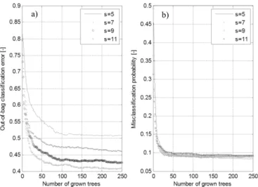
Regarding Model II, the number of randomly selected features (s=11) is different from Model I. For Model II, Fig. 2(a) suggests higher values of s for minimizing the out-of-bag classification error. However, Fig. 2(b) indicates that the parameter hasn’t any influence on the misclassification probability.
Fig. 1. (a) OOB classification error and (b) misclassification probability for Model I
a) b)
6 I. Saadi et al. / Transportation Research Procedia 00 (2017) 000–000
For both models (Fig. 1-2), we can see that errors have been significantly reduced by mitigating the variance defined in Equ. 1. In this regard, RF clearly plays an effective role.
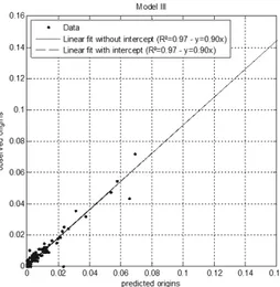
Fig. 3 plots the difference between the predicted and the observed number of OD trips in terms of R². Calibration of Model II seems correct from R²-values point of view as well as the slopes. The outputs predicted by Model I present lower slopes although the R²-values are almost close to one. However, globally, Model II behaves better that Model I when both indicators are considered. Note that in Model II, the information about trip origin has been included as a feature. Thus, the predicted trip destinations are more accurately estimated by Model II. This simulation proves that spatial information regarding trips can improve the level of accuracy of a model. Including only socio-demographic and travel behavior related features are not sufficient to ensure that the model reach good performances. The introduction of the trip destinations information as predictor clearly improves the accuracy of Model III (Fig. 4) while its absence almost reduces the slope by 50% (Fig. 3(a)).
Fig. 2. (a) OOB classification error and (b) misclassification probability for Model II
Fig. 3. (a) Fit between the predicted and observed trip origins without spatial feature – (b) Fit between the predicted and observed trip destinations with trip origins as spatial feature
a) b)
4. Results
Fig. 1(a-b) plots respectively the out-of-bag (OOB) classification error and the misclassification error found by the RF for all iterations. Cross-validation is not mandatory to assess the performance of the model and to get an unbiased estimate of the validation dataset error. Indeed, during the simulation, trees are grown according to their respective bootstraps. All the remaining features (non-selected features of the random subspace method) can be used as test sets. In this context, OOB classification error is the proportion of the instances that the outcome differs from the true class. In contrast, the determination of the error by means of misclassification probabilities is slightly different from the previous method. Here, the idea consists in defining a large number of independent test data. Then the probability estimates are determined within each test data, so that the misclassification error rate is computed across all the individual test data sets.
In the first model, we didn’t include deliberately the feature information regarding the spatial information (i.e. destination), thus an OOB error of 66% is obtained for the best value of s (number of selected features). Conversely, in Model II (Fig. 3(b)) and Model III (Fig. 4), for estimating respectively the trip destinations and the trip origins, their related spatial features have been taken into account. In this regard, the OOB error was almost reduced until 42%. This difference of errors clearly shows that including spatial information as predictors increase the accuracy of RF model.
We run the simulations for different values of the randomly selected features to assess the influence of this tuning parameter on the errors. The results clearly indicate that, regarding Model I, both errors are minimized for s=4.
Furthermore, we can conclude that the algorithm is almost converging after 150 grown trees. In the beginning, the number of trees is low so the second term of the variance equation of RF
2
1
T
(3)
contributes significantly to both errors assessment. Furthermore, despite the fact that the standard value proposed by Breiman (2001) for the number of randomly selected features should be n/3, it is better to make a sensitivity analysis to find the most correct value of s.
Regarding Model II, the number of randomly selected features (s=11) is different from Model I. For Model II, Fig. 2(a) suggests higher values of s for minimizing the out-of-bag classification error. However, Fig. 2(b) indicates that the parameter hasn’t any influence on the misclassification probability.
Fig. 1. (a) OOB classification error and (b) misclassification probability for Model I
a) b)
For both models (Fig. 1-2), we can see that errors have been significantly reduced by mitigating the variance defined in Equ. 1. In this regard, RF clearly plays an effective role.
Fig. 3 plots the difference between the predicted and the observed number of OD trips in terms of R². Calibration of Model II seems correct from R²-values point of view as well as the slopes. The outputs predicted by Model I present lower slopes although the R²-values are almost close to one. However, globally, Model II behaves better that Model I when both indicators are considered. Note that in Model II, the information about trip origin has been included as a feature. Thus, the predicted trip destinations are more accurately estimated by Model II. This simulation proves that spatial information regarding trips can improve the level of accuracy of a model. Including only socio-demographic and travel behavior related features are not sufficient to ensure that the model reach good performances. The introduction of the trip destinations information as predictor clearly improves the accuracy of Model III (Fig. 4) while its absence almost reduces the slope by 50% (Fig. 3(a)).
Fig. 2. (a) OOB classification error and (b) misclassification probability for Model II
Fig. 3. (a) Fit between the predicted and observed trip origins without spatial feature – (b) Fit between the predicted and observed trip destinations with trip origins as spatial feature
a) b)
2572 I. Saadi et al. / Transportation Research Procedia 00 (2017) 000–000 Ismaïl Saadi et al. / Transportation Research Procedia 25 (2017) 2566–2573 7
5. Discussion and Conclusion
In this paper, we propose a RF based approach for estimating OD matrices using travel surveys. Most of the existing strategies adopt daily traffic counts for estimating O-D pairs, although using traffic counts can present some limitations. For example, it is almost impossible to cover all the road segments due to practical and economic considerations. Thus, shifting towards other alternatives is necessary especially in the context of countries where such data are difficult to obtain.
In this study, we have opted for a travel survey to calibrate the O-D matrix. As stated by Cools et al. (2010), travel surveys may contain important errors emanating from the sampling variance. In this context, we proposed a RF approach, as it is characterized by its capacity to mitigate the variance. Also, there is no risk of overfitting because of the merging between random subspace method and bagging principles.
The preliminary results are quite encouraging although some improvements are necessary regarding relevant features selection and calibration of the models. Furthermore, although the obtained O-D matrix has been validated with regard to the test sets, validation of the models can be fully ensured only when a comparison with traffic measurements will be done. In this regard, further research should be carried out with respect to model validation.
Acknowledgements
The research was funded through the ARC grant for Concerted Research Actions financed by the Wallonia-Brussels Federation.
References
Amit, Y., Geman, D., 1997. Shape Quantization and Recognition with Randomized Trees. Neural Comput. 9, 1545–1588. doi:10.1162/neco.1997.9.7.1545
Ashok, K., Ben-Akiva, M.E., 2002. Estimation and Prediction of Time-Dependent Origin-Destination Flows with a Stochastic Mapping to Path Flows and Link Flows. Transp. Sci. 36, 184–198. doi:10.1287/trsc.36.2.184.563
Bell, M.G.H., 1983. The Estimation of an Origin-Destination Matrix from Traffic Counts. Transp. Sci. 17, 198–217. doi:10.1287/trsc.17.2.198 Bera, S., Rao, K.V.K., 2011. Estimation of origin-destination matrix from traffic counts: the state of the art. Eur. Transp. Trasp. Eur. 2–23. Breiman, L., 2001. Random Forests. Mach. Learn. 45, 5–32. doi:10.1023/A:1010933404324
Breiman, L., 1996. Bagging predictors. Mach. Learn. 24, 123–140. doi:10.1007/BF00058655
Cascetta, E., 1984. Estimation of trip matrices from traffic counts and survey data: A generalized least squares estimator. Transp. Res. Part B Methodol. 18, 289–299. doi:10.1016/0191-2615(84)90012-2
Cools, M., Moons, E., Wets, G., 2010. Assessing the Quality of Origin-Destination Matrices Derived from Activity Travel Surveys. Transp. Res. Rec. J. Transp. Res. Board 2183, 49–59. doi:10.3141/2183-06
Fig. 4. Fit between the predicted and observed origins with trip destinations as spatial feature
8 I. Saadi et al. / Transportation Research Procedia 00 (2017) 000–000
Djukic, T., van Lint, H., Hoogendoorn, S.P., 2014. Methodology for efficient real time OD demand estimation on large scale networks. Presented at the Transportation Research Board 93rd Annual Meeting.
Flötteröd, G., Bierlaire, M., Nagel, K., 2011. Bayesian Demand Calibration for Dynamic Traffic Simulations. Transp. Sci. 45, 541–561. doi:10.1287/trsc.1100.0367
Frederix, R., Viti, F., Himpe, W.W.E., Tampère, C.M.J., 2014. Dynamic Origin–Destination Matrix Estimation on Large-Scale Congested Networks Using a Hierarchical Decomposition Scheme. J. Intell. Transp. Syst. 18, 51–66. doi:10.1080/15472450.2013.773249 Frederix, R., Viti, F., Tampère, C.M.J., 2013. Dynamic origin–destination estimation in congested networks: theoretical findings and implications
in practice. Transp. Transp. Sci. 9, 494–513. doi:10.1080/18128602.2011.619587
Hastie, T., Tibshirani, R., Friedman, J., 2009. Random Forests, in: The Elements of Statistical Learning, Springer Series in Statistics. Springer New York, pp. 587–604.
Ho, T.K., 1995. Random decision forests, in: , Proceedings of the Third International Conference on Document Analysis and Recognition, 1995. Presented at the , Proceedings of the Third International Conference on Document Analysis and Recognition, 1995, pp. 278–282 vol.1. doi:10.1109/ICDAR.1995.598994
Lorenzo, M., Matteo, M., 2013. OD Matrices Network Estimation from Link Counts by Neural Networks. J. Transp. Syst. Eng. Inf. Technol. 13, 84–92. doi:10.1016/S1570-6672(13)60117-8
Maher, M.J., 1983. Inferences on trip matrices from observations on link volumes: A Bayesian statistical approach. Transp. Res. Part B Methodol. 17, 435–447. doi:10.1016/0191-2615(83)90030-9
Marzano, V., Papola, A., Simonelli, F., 2009. Limits and perspectives of effective O–D matrix correction using traffic counts. Transp. Res. Part C Emerg. Technol., Selected papers from the Sixth Triennial Symposium on Transportation Analysis (TRISTAN VI) 17, 120–132. doi:10.1016/j.trc.2008.09.001
Perrakis, K., Karlis, D., Cools, M., Janssens, D., 2015. Bayesian inference for transportation origin–destination matrices: the Poisson–inverse Gaussian and other Poisson mixtures. J. R. Stat. Soc. Ser. A Stat. Soc. 178, 271–296. doi:10.1111/rssa.12057
Perrakis, K., Karlis, D., Cools, M., Janssens, D., Vanhoof, K., Wets, G., 2012. A Bayesian approach for modeling origin–destination matrices. Transp. Res. Part Policy Pract. 46, 200–212. doi:10.1016/j.tra.2011.06.005
Sammut, C., Webb, G.I., 2011. Encyclopedia of Machine Learning, 1st ed. Springer Publishing Company, Incorporated. Stopher, P.R., Greaves, S.P., 2007. Household travel surveys: Where are we going? Transp. Res. Part Policy Pract. 41, 367–381.
doi:10.1016/j.tra.2006.09.005
Talebian, A., Shafahi, Y., 2015. The treatment of uncertainty in the dynamic origin–destination estimation problem using a fuzzy approach. Transp. Plan. Technol. 38, 795–815. doi:10.1080/03081060.2015.1059124
Toledo, T., Kolechkina, T., 2013. Estimation of Dynamic Origin #x2013;Destination Matrices Using Linear Assignment Matrix Approximations. IEEE Trans. Intell. Transp. Syst. 14, 618–626. doi:10.1109/TITS.2012.2226211
5. Discussion and Conclusion
In this paper, we propose a RF based approach for estimating OD matrices using travel surveys. Most of the existing strategies adopt daily traffic counts for estimating O-D pairs, although using traffic counts can present some limitations. For example, it is almost impossible to cover all the road segments due to practical and economic considerations. Thus, shifting towards other alternatives is necessary especially in the context of countries where such data are difficult to obtain.
In this study, we have opted for a travel survey to calibrate the O-D matrix. As stated by Cools et al. (2010), travel surveys may contain important errors emanating from the sampling variance. In this context, we proposed a RF approach, as it is characterized by its capacity to mitigate the variance. Also, there is no risk of overfitting because of the merging between random subspace method and bagging principles.
The preliminary results are quite encouraging although some improvements are necessary regarding relevant features selection and calibration of the models. Furthermore, although the obtained O-D matrix has been validated with regard to the test sets, validation of the models can be fully ensured only when a comparison with traffic measurements will be done. In this regard, further research should be carried out with respect to model validation.
Acknowledgements
The research was funded through the ARC grant for Concerted Research Actions financed by the Wallonia-Brussels Federation.
References
Amit, Y., Geman, D., 1997. Shape Quantization and Recognition with Randomized Trees. Neural Comput. 9, 1545–1588. doi:10.1162/neco.1997.9.7.1545
Ashok, K., Ben-Akiva, M.E., 2002. Estimation and Prediction of Time-Dependent Origin-Destination Flows with a Stochastic Mapping to Path Flows and Link Flows. Transp. Sci. 36, 184–198. doi:10.1287/trsc.36.2.184.563
Bell, M.G.H., 1983. The Estimation of an Origin-Destination Matrix from Traffic Counts. Transp. Sci. 17, 198–217. doi:10.1287/trsc.17.2.198 Bera, S., Rao, K.V.K., 2011. Estimation of origin-destination matrix from traffic counts: the state of the art. Eur. Transp. Trasp. Eur. 2–23. Breiman, L., 2001. Random Forests. Mach. Learn. 45, 5–32. doi:10.1023/A:1010933404324
Breiman, L., 1996. Bagging predictors. Mach. Learn. 24, 123–140. doi:10.1007/BF00058655
Cascetta, E., 1984. Estimation of trip matrices from traffic counts and survey data: A generalized least squares estimator. Transp. Res. Part B Methodol. 18, 289–299. doi:10.1016/0191-2615(84)90012-2
Cools, M., Moons, E., Wets, G., 2010. Assessing the Quality of Origin-Destination Matrices Derived from Activity Travel Surveys. Transp. Res. Rec. J. Transp. Res. Board 2183, 49–59. doi:10.3141/2183-06
Fig. 4. Fit between the predicted and observed origins with trip destinations as spatial feature
Djukic, T., van Lint, H., Hoogendoorn, S.P., 2014. Methodology for efficient real time OD demand estimation on large scale networks. Presented at the Transportation Research Board 93rd Annual Meeting.
Flötteröd, G., Bierlaire, M., Nagel, K., 2011. Bayesian Demand Calibration for Dynamic Traffic Simulations. Transp. Sci. 45, 541–561. doi:10.1287/trsc.1100.0367
Frederix, R., Viti, F., Himpe, W.W.E., Tampère, C.M.J., 2014. Dynamic Origin–Destination Matrix Estimation on Large-Scale Congested Networks Using a Hierarchical Decomposition Scheme. J. Intell. Transp. Syst. 18, 51–66. doi:10.1080/15472450.2013.773249 Frederix, R., Viti, F., Tampère, C.M.J., 2013. Dynamic origin–destination estimation in congested networks: theoretical findings and implications
in practice. Transp. Transp. Sci. 9, 494–513. doi:10.1080/18128602.2011.619587
Hastie, T., Tibshirani, R., Friedman, J., 2009. Random Forests, in: The Elements of Statistical Learning, Springer Series in Statistics. Springer New York, pp. 587–604.
Ho, T.K., 1995. Random decision forests, in: , Proceedings of the Third International Conference on Document Analysis and Recognition, 1995. Presented at the , Proceedings of the Third International Conference on Document Analysis and Recognition, 1995, pp. 278–282 vol.1. doi:10.1109/ICDAR.1995.598994
Lorenzo, M., Matteo, M., 2013. OD Matrices Network Estimation from Link Counts by Neural Networks. J. Transp. Syst. Eng. Inf. Technol. 13, 84–92. doi:10.1016/S1570-6672(13)60117-8
Maher, M.J., 1983. Inferences on trip matrices from observations on link volumes: A Bayesian statistical approach. Transp. Res. Part B Methodol. 17, 435–447. doi:10.1016/0191-2615(83)90030-9
Marzano, V., Papola, A., Simonelli, F., 2009. Limits and perspectives of effective O–D matrix correction using traffic counts. Transp. Res. Part C Emerg. Technol., Selected papers from the Sixth Triennial Symposium on Transportation Analysis (TRISTAN VI) 17, 120–132. doi:10.1016/j.trc.2008.09.001
Perrakis, K., Karlis, D., Cools, M., Janssens, D., 2015. Bayesian inference for transportation origin–destination matrices: the Poisson–inverse Gaussian and other Poisson mixtures. J. R. Stat. Soc. Ser. A Stat. Soc. 178, 271–296. doi:10.1111/rssa.12057
Perrakis, K., Karlis, D., Cools, M., Janssens, D., Vanhoof, K., Wets, G., 2012. A Bayesian approach for modeling origin–destination matrices. Transp. Res. Part Policy Pract. 46, 200–212. doi:10.1016/j.tra.2011.06.005
Sammut, C., Webb, G.I., 2011. Encyclopedia of Machine Learning, 1st ed. Springer Publishing Company, Incorporated. Stopher, P.R., Greaves, S.P., 2007. Household travel surveys: Where are we going? Transp. Res. Part Policy Pract. 41, 367–381.
doi:10.1016/j.tra.2006.09.005
Talebian, A., Shafahi, Y., 2015. The treatment of uncertainty in the dynamic origin–destination estimation problem using a fuzzy approach. Transp. Plan. Technol. 38, 795–815. doi:10.1080/03081060.2015.1059124
Toledo, T., Kolechkina, T., 2013. Estimation of Dynamic Origin #x2013;Destination Matrices Using Linear Assignment Matrix Approximations. IEEE Trans. Intell. Transp. Syst. 14, 618–626. doi:10.1109/TITS.2012.2226211