CAN EDDY-COVARIANCE BE USED ON A PASTURE? ESTIMATION OF CATTLE AND SOIL- PLANT METHANE EMISSIONS AND TRANSFER TO OTHER GREENHOUSE GASES.

COMMUNAUTÉ FRANÇAISE DE BELGIQUE UNIVERSITÉ DE LIÈGE – GEMBLOUX AGRO-BIO TECH

CAN EDDY-COVARIANCE BE USED ON A

PASTURE?

ESTIMATION OF CATTLE AND SOIL- PLANT METHANE

EMISSIONS AND TRANSFER TO OTHER GREENHOUSE

GASES.

Pierre DUMORTIER

Dissertation originale présentée en vue de l’obtention du grade de docteur en sciences agronomiques et ingénierie biologique

Promoteurs: Marc AUBINET & Bernard HEINESCH Année civile: 2020

DUMORTIER Pierre (2020). Can eddy-covariance be used on a pasture? Estimation of cattle and soil- plant methane emissions and transfer to other greenhouse gases. PhD Thesis. Université de Liège - Gembloux Agro-Bio Tech, Belgium. 174 p.

vi

Abstract

Much debate has arisen as to the contribution of natural and anthropized ecosystems to the global production of greenhouse gases (GHG), ways to limit this contribution or how to use ecosystems as carbon sinks. To provide solid ground for this debate, reliable data is required. Eddy-covariance (EC) is commonly used to measure gaseous exchanges from homogeneous ecosystems (crops, forests…). However, in its standard form, it may be biased when working with heterogeneous ecosystems, especially grazed pastures where cattle is an important, but also moving and intermittent GHG source. In this thesis, using data from the Dorinne ecosystem station, a Belgian pasture grazed by Belgian Blue beef, we disentangled cattle methane (CH4) and carbon

dioxide (CO2) exchanges from soil-plant exchanges. This work allowed us estimate

cattle CH4 and CO2 emissions and compute an un-biased pasture GHG budget. Our

work therefore opens the door to a wider use of EC on grazed pastures and thus the monitoring of this important ecosystem.

In practice, EC measures gaseous exchanges from an area upwind from the measurement mast. Each area contribution to the measured flux can be computed using a mathematical model (footprint model). We combined this footprint model with cattle positions on the pasture, obtained using GPS-collars, and EC in order to estimate cattle CH4 emissions. The proposed method was validated through an

artificial tracer experiment where source recovery rates were between 90 and 113% and no bias was associated with atmospheric conditions or the distance between the source and the measurement mast. Applying this validated method on grazing Belgian Blue cows led to estimated CH4 emissions of 220 ± 35 gCH4 head−1 day−1. Cow’s

behavior was also monitored and presented a clear daily pattern of activity with more intense grazing just after sunrise and right before sunset. However, no significant CH4

emission pattern could be associated with it, indicating that the diurnal emission variation might be lower than the measurement uncertainty range.

We extended our method to cattle CO2 emissions. To avoid the need for cattle

geolocation, we used CH4 fluxes as an indicator of cattle presence in the footprint.

This allowed us by-passing labor intensive handling of cattle, thus making our method easier to use on a large number of test sites. Using this method, estimated cow CO2

emissions were of 3.2 ± 0.5 kgC head−1 day−1. Moreover, we computed a pasture GHG emission (CO2, CH4 and N2O) of 629 ± 296 gCO2eq m−2 yr-1. This figure should be

handled with some precautions as it is site specific, dependent on budget boundaries and subject to annual variations.

Key words: Methane, Carbon dioxide, Pasture, Eddy covariance, Cattle, Footprint, Geolocation.

vii

Résumé

La contribution des écosystèmes naturels et anthropisés à la production mondiale de gaz à effet de serre (GES), les façons de limiter cette contribution et l’utilisation des écosystèmes comme puits de carbone fait l’objet de nombreux débats. Pour fournir une base solide à ce débat, des données fiables sont nécessaires. La covariance des turbulences (CT) est couramment utilisée pour mesurer les échanges gazeux provenant d'écosystèmes homogènes (cultures, forêts…). Cependant, dans sa forme standard, elle peut être biaisée lorsque l'on travaille avec des écosystèmes hétérogènes, en particulier les pâturages où le bétail est une source de GES importante, mais aussi une source mobile et intermittente. Dans cette thèse, en utilisant les données de la station écosystème de Dorinne, un prairie belge pâturée par du bétail blanc bleu belge, nous avons séparés les échanges de méthane (CH4) et de dioxyde de carbone (CO2)

des bovins des échanges sol-plante. Ce travail nous a permis d'estimer les émissions de CH4 et de CO2 par animal ainsi que de calculer correctement le bilan de GES de

cette pâture. Notre travail ouvre la porte à une utilisation plus large de la CT sur les pâturages et donc au suivi de cet écosystème important.

En pratique, la CT mesure les échanges gazeux provenant d'une zone en amont du mât de mesure par rapport au vent. Chaque contribution de surface au flux mesuré peut être calculée à l'aide d'un modèle mathématique (modèle d’empreinte). Nous avons combiné ce modèle d’empreinte avec les positions du bétail sur le pâturage, obtenues à l'aide de colliers GPS, et la CT afin d'estimer leurs émissions de CH4. La

méthode proposée a été validée par une expérience avec traceur artificiel où les taux de récupération se situaient entre 90 et 113%. De plus, aucun biais n'était associé aux conditions atmosphériques ou à la distance entre la source et le mât de mesure. L'application de cette méthode validée aux vaches blanc bleues belges au pâturage a conduit à des émissions de CH4 estimées de 220 ± 35 gCH4 tête-1 jour-1. Le

comportement des vaches a également été surveillé et présentait un schéma d'activité quotidien clair avec un pâturage plus intense juste après le lever du soleil et juste avant le coucher du soleil. Cependant, aucune corrélation significative avec les émissions de CH4 n'a pu lui être associé, ce qui indique que la variation diurne des émissions

pourrait être inférieure à la plage d'incertitude de mesure.

Nous avons étendu notre méthode aux émissions de CO2 des bovins. Pour éviter le

besoin de géolocalisation du bétail, nous avons utilisé les flux de CH4 comme

indicateurs de la présence du bétail dans l’empreinte. Cela nous a permis d’éviter toute manipulation du bétail, rendant ainsi notre méthode plus facile à utiliser sur un grand nombre de sites. En utilisant cette méthode, les émissions de CO2 estimées des vaches

étaient de 3,2 ± 0,5 kgC tête-1 _jour-1_{. De plus, nous avons calculé un bilan de GES de}

notre pâture (CO2, CH4 et N2O) de 629 ± 296 gCO2eq m−2 an-1. Ce chiffre doit être

manipulé avec quelques précautions car il est spécifique au site, dépendant des frontières du système et est sujet a des variations annuelles.

viii

Acknowledgment/ Remerciements

Alors là, je ne sais pas trop par où commencer ; tellement de personnes m’ont entourées pendant ces longues années. Promoteurs, membres du comité de thèse ou du jury, collègues et anciens collègues, étudiants de toutes années et de tout niveau, famille, amis qui ne sont pas déjà présents dans les catégories précédentes (il y en a quand même), j’ai ici une pensée pour vous tous.

Quand je pense à ma thèse je pense bien sûr tout d’abord à mes promoteurs ; Marc Aubinet et Bernard Heinesch. Ils ont toujours accepté de m’aider dans mon travail, jusque tard dans la nuit s’il le fallait. Je ne leur ai pas toujours donné une vie facile et les ai parfois fait douter. Ils n’ont pas cessé de m’encourager pour autant et je les en remercie du fond du cœur.

Je pense aussi à mes collègues avec qui j’ai passé d’excellents moments, qu’ils soient impliqués dans ma thèse, ou pas, qu’ils soient techniciens, assistants, professeurs, chercheurs, administratifs ou autres, qu’ils travaillent encore à la fac ou qu’ils soient passés par là il y a des années. Vraiment de très bons moments. Et chaque jour de travail, ou presque, était un plaisir. Je ne ferai pas ici la liste de tous ces collègues, ce serait trop long, et je prendrai bien trop de risque à oublier un nom, cela m’arrive si souvent. Je dirai juste que j’aimerais vous voir et vous revoir encore peu importe l’endroit où je travaille. Je vais quand même prendre le temps de parler de ceux qui ont contribué directement à ma thèse c’est-à-dire Naina Andiramandoroso, Louis Gourlez de la Motte, Nicolas De Cock et Quentin Hurdebise ; sans leurs contributions ma thèse n’aurait jamais évolué vers ce qu’elle est actuellement.

Je pense aussi tout particulièrement à Adrien Paquet qui, en plus de nous accueillir sur sa prairie, à toujours eu à cœur de nous aider, notamment par des discussions riches d’enseignements ou dans le placement des colliers GPS sur le bétail, étape indispensable à ma thèse, qui aurait été impossible sans sa contribution.

Je pense ensuite à ma famille et à mes amis dont la contribution est plus difficile à cerner et pourtant essentielle. C’est vous qui avez entretenu ma bonne humeur au quotidien, vous qui m’avez poussé à avancer et à profiter de chaque instant. Je remercie tout particulièrement Hélène Cawoy et Claude Cawoy dont les relectures et les conseils ont grandement amélioré la lisibilité du document final.

Finalement, c’est en pensant à mon promoteur de TFE, Jean-Marie Parmentier, que j’ai voulu écrire ce poème :

ix Ode à mes compagnons de route

A Bernard & Marc, je lance mes premiers mots, Vous qui avez guidé mes mains et permis l’ouvrage, Sans vous, jamais je n’aurais pu sortir de tels joyaux, Ce sont vos sourires qui m’en ont donné le courage, Aux membres du comité avec qui tout a débuté, Durant toutes ces années vous m’avez beaucoup aidé, Je vous ai fait douter, je vous ai fait espérer,

Les données ont parlé, et se préparent à lancer de nouveaux rameaux. Aux collègues je prête toutes mes pensées,

Que de plaisirs au bureau ou ailleurs au besoin, Ces belles journées que vous avez éclairées, Sans vous je n’aurais jamais été aussi loin. A ma famille vont mes sentiments les plus doux, A vous qui m’avez chéri, pouponné, cajolé,

Jamais je n’aurais pu espérer tant d’attention, un amour fou, Sans vous je n’aurais même jamais commencé.

A vous, compagnons de tout poil,

Vous qui m’avez marqué, pour toujours et à jamais, Plus que vous ne le percevez, vos actes m’ont touché, Je voudrais ici vous remercier pour tout ce que vous avez fait.

xi

Table of contents

A

BSTRACT

...

VI

R

ÉSUMÉ

...

VII

A

CKNOWLEDGMENT

/

R

EMERCIEMENTS

...

VIII

T

ABLE OF CONTENTS

...

XI

L

IST OF

F

IGURES

...

XVI

L

IST OF

T

ABLES

...

XXI

L

IST OF ACRONYMS

...

XXIII

C

HAPTER

1.

I

NTRODUCTION

... 29

A

NTHROPOGENIC GREENHOUSE GAS EMISSIONS AND CLIMATE CHANGE

... 29

C

ATTLE METHANE EMISSIONS

... 31

C

ATTLE METHANE EMISSION MEASUREMENT

... 33

C

HALLENGES ASSOCIATED WITH THE USE OF EDDY COVARIANCE ON A PASTURE

... 35

R

EMOVING TEMPORAL TRENDS

... 36

H

OMOGENEOUS CATTLE DISTRIBUTION HYPOTHESIS

... 37

H

ETEROGENEOUS CATTLE DISTRIBUTION HYPOTHESIS

... 37

S

ITE DESCRIPTION

... 38

O

BJECTIVES

... 42

P

ERSONNAL CONTRIBUTION TO THE RESEARCH PRESENTED IN THIS MANUSCRIPT

... 43

C

HAPTER

2.

M

ETHANE BALANCE OF AN INTENSIVELY GRAZED PASTURE AND ESTIMATION OF THE ENTERIC METHANE EMISSIONS FROM CATTLE

... 47

Abstract ... 47

I

NTRODUCTION

... 47

MATERIAL

AND

METHODS ... 49

S

ITE DESCRIPTION AND CATTLE MANAGEMENT

... 49

I

NSTRUMENTATION

... 50

xii

2.2.2.

Herbage mass, cattle dry matter intake and stocking density ..

... 51

D

ATA TREATMENT

... 51

2.3.1.

General corrections ... 51

2.3.2.

Footprint correction ... 53

2.3.3.

Flux contamination by distant sources ... 53

R

ESULTS

... 55

F

OOTPRINT FUNCTION

... 55

M

ETHANE DRY MOLAR FRACTION AND FLUX EVOLUTION OVER TIME

... 56

E

NTERIC EMISSIONS

... 59

G

RASSLAND EMISSIONS AND METHANE BUDGET OF THE PARCEL

.. 62

D

ISCUSSION

... 62

E

NTERIC EMISSIONS

... 62

G

RASSLAND EXCHANGES AND COMPLETE BUDGET

... 64

C

ONCLUSIONS

... 65

A

CKNOWLEDGMENTS

... 66

C

HAPTER

3.

P

OINT SOURCE EMISSION ESTIMATION USING EDDY COVARIANCE

:

VALIDATION USING AN ARTIFICIAL SOURCE EXPERIMENT

69

Abstract ... 69

I

NTRODUCTION

... 69

M

ATERIALS

&

METHOD

... 71

S

ITE DESCRIPTION

... 71

E

XPERIMENTAL SETUP

... 72

S

OURCE EMISSION QUANTIFICATION

... 72

R

ESULTS

&

D

ISCUSSION

... 76

C

ONTAMINATION BY UNCONTROLLED SOURCES

... 76

M

ETHANE EMISSION ESTIMATION

... 77

3.2.1.

Footprint calculation method ... 79

3.2.2.

Averaging period ... 81

3.2.3.

Averaging method ... 82

xiii

S

ENSITIVITY ANALYSIS

... 82

C

ONCLUSION

... 85

A

CKNOWLEDGMENT

... 86

C

HAPTER

4.

B

EEF CATTLE METHANE EMISSION ESTIMATION USING THE EDDY

-

COVARIANCE TECHNIQUE IN COMBINATION WITH GEOLOCATION

... 89

Graphical abstract ... 89

Abstract ... 89

I

NTRODUCTION

... 90

M

ATERIAL AND METHODS

... 92

E

XPERIMENTAL SITE

... 92

P

OSITION AND BEHAVIOR MONITORING

... 94

F

LUX MEASUREMENT AND PROCESSING

... 97

2.3.1.

Enteric emission estimation ... 99

R

ESULTS

... 100

C

ATTLE BEHAVIOR AND DISTRIBUTION

... 100

E

NTERIC METHANE EMISSIONS

... 102

R

ELATIONS BETWEEN CATTLE BEHAVIOR AND EMISSIONS

... 105

C

ATTLE METHANE EMISSIONS BIAS ANALYSIS

... 107

D

ISCUSSION

... 108

V

ALIDITY OF THE METHOD

... 108

B

ELGIAN

B

LUE

CH

4 EMISISONS

... 108

I

MPACT OF CATTLE BEHAVIOR ON

CH

4 EMISSIONS

... 109

C

ONCLUSIONS

... 109

A

CKNOWLEDGMENTS

... 110

C

HAPTER

5.

H

ERD POSITION HABITS CAN BIAS NET

CO

2 ECOSYSTEM EXCHANGE ESTIMATES IN FREE RANGE GRAZED PASTURES

... 113

xiv

I

NTRODUCTION

... 114

M

ATERIAL AND METHODS

... 116

S

ITE DESCRIPTION AND GRASSLAND MANAGEMENT

... 116

F

LUX MEASUREMENTS AND PROCESSING

... 117

M

ETEOROLOGICAL MEASUREMENTS

... 117

G

ENERAL DESCRIPTION OF THE METHODOLOGY

... 117

S

TOCKING DENSITY IN THE FOOTPRINT AND ON THE PASTURE

.... 118

H

OMOGENEOUS APPROACH FOR

E

COW

... 119

H

ETEROGENEOUS APPROACHES FOR

ECOW ... 122

2.7.1.

GPS approach ... 122

2.7.2.

Confinements approach ... 123

2.7.3.

Animal carbon budget approach ... 124

A

LTERNATIVE

NEETOT

DETERMINATION

... 126

R

ESULTS

... 126

A

NIMAL POSITIONS ON THE PASTURE AND FOOTPRINT AREA

... 126

C

OW RESPIRATION RATE PER

LU

CONSIDERING A HOMOGENEOUS COW REPARTITION

... 128

3.2.1.

Validation of the CH

4

flux filtering approach ... 128

3.2.2.

Discriminating NEE

tot

into NEE

past

and R

cows

... 130

3.2.3.

Cow respiration rate per LU (E

cow,hom

) ... 130

C

OW RESPIRATION RATE PER

LU

WITH CONSIDERING HETEROGENEOUS COW REPARTITION

... 131

3.3.1.

GPS trackers (E

cow,GPS

) ... 131

3.3.2.

Confinement experiments (E

cow,conf

) ... 132

3.3.3.

Animal scale carbon budget (E

cow,budg

) ... 132

B

IAS INDUCED BY A NON

-

HOMOGENEOUS COW DISTRIBUTION

... 133

D

ISCUSSION

... 135

U

SING METHANE FLUXES AS A

NEETOT

PARTITION TOOL

... 135

B

IASED

NEE

ESTIMATES BECAUSE OF A NON

-

HOMOGENEOUS COW REPARTITION

... 135

M

ETHOD TO MEASURE A REFERENCE COW RESPIRATION RATE PER

LU

... 136

C

ONCLUSIONS AND RECOMMENDATIONS

... 137

xv

C

HAPTER

6.

G

ENERAL DISCUSSION

,

PERSPECTIVES

&

CONCLUSIONS

... 143

E

RGODIC HYPOTHESIS

... 144

I

SSUE

... 144

C

ONTRIBUTION

... 144

O

UTLOOK

... 145

F

LUX ALLOCATION

... 145

I

SSUE

... 145

C

ONTRIBUTION

... 146

O

UTLOOK

... 147

E

MISSION ESTIMATION

... 147

I

SSUE

... 148

C

ONTRIBUTION

... 148

3.2.1.

Source density in the footprint ... 148

3.2.2.

Cattle emission estimation method ... 148

3.2.3.

Measurements at the Be-Dor ecosystem station ... 149

3.2.4.

Comparison with existing methods ... 149

O

UTLOOK

... 150

D

RIVERS

... 151

I

SSUE

... 151

C

ONTRIBUTION

... 151

O

UTLOOK

... 152

GHG

BUDGET

... 152

I

SSUE

... 152

C

ONTRIBUTION

... 152

O

UTLOOK

... 154

C

ONCLUSIONS

... 154

R

EFERENCES

... 159

xvi

List of Figures

Figure 1-1: Global average near surface temperature annual anomalies since the pre-industrial period (HadCRUT4: Met Office Hadley Centre and Climatic Research Unit, GISTEMP: NASA Goddard Institute for Space Studies, NOAA Global Temp: National Centers for Environment) Credits: (European Environment Agency, 2020). ... 30

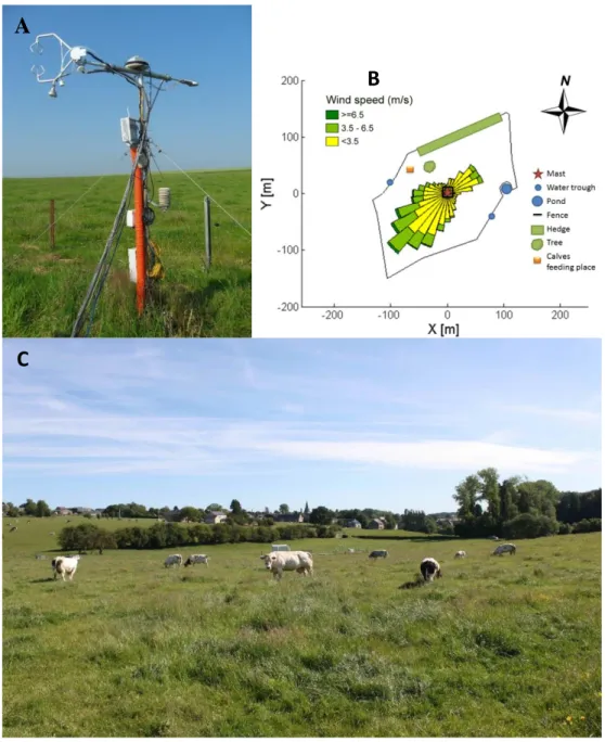
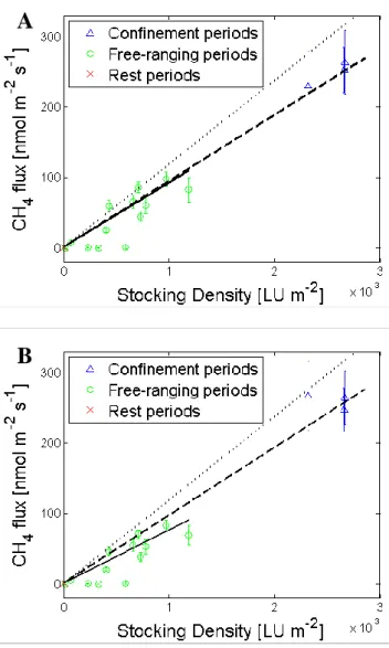
Figure 1-2: The global greenhouse gas emissions, per type of gas and source, including LULUCF. F- gases stands for fluorinated GHG. Credits: Olivier J.G.J. and Peters J.A.H.W. (2018), Trends in global CO2 and total greenhouse gas emissions: 2018 report. PBL. Netherlands Environmental Assessment Agency. ... 31 Figure 1-3: Rumen metabolic pathways. Credits : (Haque, 2018). ... 32 Figure 1-4: Satellite view from the Dorinne Ecosystem Station. The pasture is highlighted in white, the red cross indicates the mast and the ellipse indicate the barn location. Credits: Google earth. ... 39 Figure 1-5: Measurement mast with sonic anemometer and sampling tube (A), schematic view of the pasture with main wind directions and velocities overlaid on the mast location (B) and general view of the site, the instrumentation being partly hidden by the white cow. ... 41 Figure 2-1: Stocking density evolution throughout the measuring period; the periods with stocking densities above 15 10-4 _{LU m}−2 _{correspond to confinement}

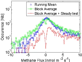
periods. ... 49 Figure 2-2: Schematic view of the pasture. During confinement periods, gates in internal fences were closed and the cattle were confined to the south-western part of the pasture. ... 50 Figure 2-3: Methane flux occurrence distribution for three data treatment methods. Data were filtered for low friction velocity (u*) and signal contamination (see text).

For better readability, only fluxes between -10 and 10 nmol m−2 s−1 are shown. ... 52 Figure 2-4: Scatterplot of methane fluxes vs u* during rest periods. Fluxes are

filtered for contamination by distant sources (see text). For better readability, only fluxes between -5 and 5 nmol m−2 s−1 and u* values below 0.7 are shown. Crosses

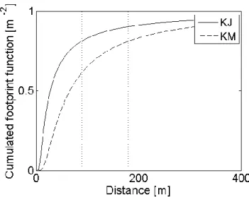
correspond to bin averages on one tenth of the half-hours each. Error bars correspond to the 95% confidence interval. ... 53 Figure 2-5: Directional intensity of methane fluxes (nmol m−2 s−1) during rest periods in winter (dark blue) and during growing season (light red). The circle is centered on the measurement mast. The barn is indicated by the black dot, 350 m north-east (30° N, clockwise) of the mast. ... 54 Figure 2-6: Cumulated footprint function along the main wind direction for June 09 2013 at 6:00 u*= 0.25 m s−1, z/L=-0.036). Dotted lines indicate the shortest

(north-west) and longest (south-(north-west) distances between the mast and the border of the paddock. ... 56

xvii

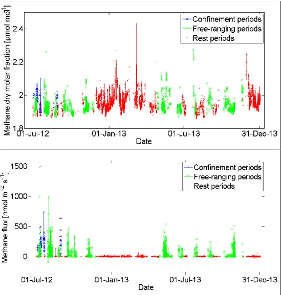
Figure 2-7: Evolution over time of methane dry molar fraction (A) and fluxes (B) using KM. Each point corresponds to a half-hour and the colors indicate level of cattle presence on the pasture. ... 57 Figure 2-8: Diurnal pattern of methane dry molar fraction (A) and fluxes (B) using the KM footprint model. Error bars correspond to standard errors of the mean. Fluxes are filtered for contamination by distant sources and for low u*, whereas methane dry

molar fractions are filtered for contamination by distant sources only. Note the use of a logarithmic scale for the vertical axis. ... 59 Figure 2-9: Relation between methane flux and stocking density. Methane fluxes are measured by eddy covariance and corrected for footprint using (A) the KM and (B) the KJ footprint model. Each point is the mean over one grazing period with constant stocking density. Only periods gathering more than 20 valid measurements are represented here. Error bars are 95% confidence intervals. The dotted line correspond to the predicted response (IPCC, 2006); solid and striped lines correspond to linear least square regressions on individual half-hours grouping rest periods and either free-ranging (R²=0.26) or confinement (R²=0.61) periods. ... 60 Figure 2-10: Average diurnal course of methane emissions per livestock unit during free-ranging periods (squares) and confinement events (triangle) calculated using (A) the KM and (B) the KJ footprint model. Error bars correspond to standard errors of the mean. Time is given in local time without daylight saving time (UTC+1). ... 61 Figure 3-1: Methane concentration evolution before (no shading) and after (shading) activation of the artificial source. ... 73 Figure 3-2: Mean measured methane flux (nmol m−2 s−1) during each campaign according to wind direction, overlaid on the map of the site. The 23 NE, 60 SW, and 80 SW campaigns only include periods with an active artificial source. The no artificial source line refers to data collected a few days before, during (with inactive artificial source), and a few days after each campaign. The dark spot indicates the barn location. ... 77 Figure 3-3: Measured methane fluxes (FCH4) according to the source contribution

to the footprint (𝜙𝑠𝑜𝑢𝑟𝑐𝑒). Each point corresponds to a 15 minutes integration period and is represented only when the artificial source is emitting. 𝜙𝑠𝑜𝑢𝑟𝑐𝑒 values were calculated using the KM (Kormann and Meixner, 2001) footprint model (A) or the FFP (Kljun et al., 2015) tool (B). Solid lines correspond to the linear least square regression line and the dotted line corresponds to the expected relation (intercept of 0 and slope equal to the real emission). Fluxes were calculated using a running mean and without application of the Foken & Wichura (1996) stationarity test. ... 80 Figure 3-4: Crosswind integrated footprint function (фj) averaged over all three

campaigns using the KM footprint model or the FFP tool. Dashed lines indicate tested distances (23, 60, and 80 m). ... 81 Figure 3-5: Impact of the distance from the mast (A), relative distance to the KM footprint peak (B), atmospheric stability parameter (z-d)/L) (C), friction velocity (u*)

(D), angular deviation between the source position and the wind direction (E), and wind direction variance (F) on the estimated methane emission (fCH4). For each

xviii

Atmospheric stability, friction velocity, angular deviation, wind speed and direction variances are organized in 5 categories containing the same number of samples and plotted at the category mean. The error bars correspond to the 95% confidence interval of the slope. The dotted line indicates the artificial source emission. ... 84 Figure 4-1: Satellite view from the Dorinne Ecosystem Station. The pasture is highlighted in white, the red cross indicates the mast and the black ellipse indicates the location of the barn. ... 93 Figure 4-2: Position and activity tracking device represented with the three axis system of the accelerometer... 95 Figure 4-3: Scatterplot of acceleration characteristics along the x-axis for a single cow and during a single measurement campaign. The horizontal axis corresponds to the mean acceleration and the vertical axis corresponds to the standard deviation. Each point represents a 20 s sample and is automatically associated with a behavior by an algorithm. ... 96 Figure 4-4: Mean cumulative footprint during the whole measurement period using the Kormann & Meixner footprint model. The isopleths represent the area responsible for x% of the measured flux (proportion of the footprint found inside a specific area). The bold line corresponds to the pasture limits. ... 98 Figure 4-5: Density maps of cows’ positions when grazing (A) or expressing other behaviors (B) for all four campaigns combined. The black line represents the limits of the pasture. The occupancy is calculated as the percentage of the time spent by cattle in each square meter. A homogeneous cattle distribution would result in a 0.06% occupancy over the whole pasture. ... 101 Figure 4-6: Average percentage of the herd grazing (green) and distance covered between each measurement (black; each 5 minutes) according to the time of day for all four campaigns combined. ... 102 Figure 4-7: Relation between measured methane flux and stocking density in the footprint (SDf) calculated according to the Kormann & Meixner footprint model for

the Spring 2014 campaign with each point corresponding to a 30-minute measurement interval. The different regression lines correspond to the reduced major axis method (RMA), the linear least square (LLS) and the median-median regression method (MMR) (see §2.3.1 for more details about each method). ... 103 Figure 4-8 Impact of the size of the dataset on methane emissions per livestock unit (fCH4) confidence intervals estimated using a bootstrapping method. For each possible

size of the dataset, 5000 sub-samples were analyzed in order to compute associated fCH4 estimates. For x% of those runs, estimated fCH4 values were found within the .x

confidence interval, x corresponding to 95 (yellow) or 50 (green). ... 105 Figure 4-9: Methane emission per livestock unit (fCH4) evolution throughout the day

for each measurement campaign computed with the reduced major axis (RMA) regression method and the Kormann & Meixner footprint model. The whiskers indicate the 95% uncertainty range of fCH4 for each 4-hour period (bootstrapping). The

green line indicates the percentage of animal grazing and the yellow strip indicates the photoperiod for this specific time of year. Whiskers are only represented when more than 10 points were available for a given interval. ... 106

xix

Figure 4-10: Methane emissions per livestock unit (fCH4) according to time since

grazing peak for all campaigns together. Times since grazing peak were organized into 3 categories containing the same number of samples and plotted as the category mean. The error bars correspond to the 95% confidence intervals of fCH4

(bootstrapping method). The dotted line indicates the fCH4 estimated using all data. All

values have been computed with the RMA regression method and the KM footprint model. ... 107 Figure 5-1: Schematic map of the site. During confinements, internal fences were closed and the cattle were confined in the south-west part of the pasture. Figure taken from Dumortier et al. (2017a). ... 116 Figure 5-2: Flow chart of the procedure used to estimate cow respiration rates per livestock unit (Ecow) using either GPS campaigns or assuming a homogeneous cow

repartition in the field (CH4 approach). Both procedures are similar, differing in their

way of assessing the presence of cows in the footprint (FP) and of assessing the stocking density (stocking density in the pasture (SDP) for the CH4 filtering approach,

or stocking density in the footprint (SDf) for the GPS method). Gaps in total net

ecosystem exchange (NEEtot) were filled only for the CH4 approach. Gaps in pasture

net ecosystem exchange (NEEpast) were filled for both approaches. Figure modified

after Felber et al., (2016b). ... 120 Figure 5-3: Illustration of the fluxes involved in the carbon (C) budget of a cow. Ecow,budg corresponds to the respiration of a cow estimated from the carbon budget, F

CH4-C the methane emitted by the cow, Cexcretions the C lost in excretions, and Cintake

the C ingested through biomass consumption. ... 125 Figure 5-4: Cow distribution maps during the GPS campaigns for both days (a) and nights (b). The same scale is used for both maps. The numeric scale of the color map is given for a comparison purpose. One unit corresponds to the presence of one animal in a pixel of 5×5m2 _{during 5 minutes. Areas colored in white are areas that are never}

visited by the herd. The average wind rose for the year 2015 is also presented both during the day (c) and during the night (d). For interpretation of the colors in this figure, the reader is referred to the electronic version of this article. ... 127 Figure 5-5: Evolution of the gap filled total cow respiration (Rcows), the net

ecosystem exchange including cow respiration (NEEtot) and the net ecosystem

exchange excluding cow respiration NEEpast for both 2013 (a) and 2015 (b). Grazing

periods are indicated in grey. (c) Evolution of stocking densities on the field for both years... 129 Figure 5-6: Mean cow respiration rates per LU in 2013 and 2015 computed from (a) all the data (Ecow,hom), (b) daylight data (Ecow,hom,day, global radiation >2.5 W m−2),

and (c) night data (Ecow,hom,night) considering a homogeneous cow repartition. Average

monthly/annual respiration rates per LU were obtained by dividing total annual/monthly cow respiration (Rcows) by monthly/annual average SDp. Annual

values are marked by lines while circle markers correspond to the monthly values. ... 131

Figure 5-7: Linear regression between the total respiration of the cows in the footprint (Rcows) on a half-hourly time scale and the weighted stocking density in the

xx

footprint (SDf). The fitted line (y = 3160x SE = 245, R2 = 0.1) corresponds to a daily

cow respiration rate of 3.2 ± 0.5 kg C LU–1 d–1. The uncertainty bound is given as 2SE. ... 132 Figure 5-8: Average daily carbon budget of a Belgian Blue beef cow. ... 133 Figure 6-1 Schematic structure of the thesis. ... 143 Figure 6-2 Boundaries of the partial GHG budget of the pasture are represented by the red dashed line. Year round soil / plant exchanges are considered, while cattle emissions are only considered when in the pasture. Adapted from Felber et al. (2016a) ... 154

xxi

List of Tables

Table 2-1: Number (and percentage) of remaining half-hours after the application of each data treatment step for the whole dataset and for the three types of cattle management. ... 55 Table 2-2: Mean fluxes, median and quartiles for each measurement period and for the two footprint calculation models (nmol m−2 s−1). ... 58 Table 3-1: Performance score calculation method. ... 76 Table 3-2: Performance indicators for each of the 24 tested computation methods. The 24 combinations correspond to two footprint models: the one from Kormann and Meixner (2001) and a flux footprint prediction tool (FFP) developed by Kljun et al. (2015) raging (BA) and moving average using a time constant of 120 s (MA120) The combination associated with the higher performance score is highlighted in light grey. ... 78

Table 4-1: Description of the four measurement campaigns. ... 94 Table 4-2: Confusion matrix of the behavior detection algorithm. Each row of the matrix represents the instances in a predicted class while each column represents the instances in an observed class. ... 96 Table 4-3: Number (and percentage) of half-hours remaining after the application of each filtering step for each measurement campaign. ... 99 Table 4-4: Estimated cattle emissions per livestock unit (fCH4) for each campaign

using different methods: reduced major axis regression (RMA), median-median regression (MMR) or assuming a homogeneous cattle distribution. All estimations are presented through a 95% confidence interval and a 95% uncertainty range. ... 104 Table 5-1: Sources of uncertainties for annual Rcows values. Values are provided in

g C m−2 yr−1 but are accounted only during grazing period. Random error (2σ) on NEEpast and NEEtot were computed by adding some random noise in the data during

grazing periods only. The error due to the additional gaps in NEEpast was computed

by randomly adding gaps in NEEpast data set. The uncertainty or Rcows (2σ) was

computed by combining the different error terms following Gaussian error propagation. ... 122 Table 5-2: Description of the GPS campaigns. ... 123 Table 5-3: Comparison of the average stocking densities on the pasture (SDp) with

the average stocking density in the footprint (SDf) for the GPS measurement

campaigns. The averages calculated are for all data from all campaigns combined. ... 128

Table 5-4: Gap filled net ecosystem exchange of the pasture without cow influence (NEEpast) using the CH4 cow presence filtering criterion and the GPS criterion for each

GPS campaign. ... 129 Table 5-5: Number of valid net ecosystem exchange measurements, including the cow respiration rate (NEEtot) and excluding it (NEEpast), annual gap filled sums of both

xxii

net ecosystem exchange and the total gap filled annual respiration Rcows for both 2013

and 2015. Note that error bar on Rcows are not the combination of the error bars on

annual NEEtot and NEEpast (see section 2.6). ... 130

Table 5-6: Average footprint contribution of the pasture and stocking density on the pasture (SDp), daily average cow respiration rates per livestock unit (LU) computed from a) annual gap filled data sets assuming a homogeneous cow repartition on the field from day (global radiation > 2.5 W m−2, Ecow,hom,day), night (Ecow,hom,night),

and all the data (Ecow,hom) and b) without assuming this cow repartition and using GPS

trackers (Ecow,GPS), confinement experiments (Ecow,conf), and the carbon budget of the

animal (Ecow, budg). Field scale cow respiration rates are also given when computed

from the CH4 partitioning (Rcows) and when upscaled using Ecow,GPS (Rcows,GPS). The

footprint is expressed as the percentage of the flux that comes from the field on average for each year according to the KM model. ... 134 Table 6-1 Pasture GHG budget for the Be-Dor ecosystem station. Figures are relative to the years 2013 to 2019 according to the considered GHG. Budget boundaries are described in Figure 6-2. ... 153

xxiii

List of acronyms

BA Block averaging method BE-Dor Dorinne ecosystem station

C Carbon

CH4 Methane

CO2 Carbon dioxide

DMI Dry matter intake

DTO Dorinne Terrestrial Observatory

EC Eddy covariance

Ecow Estimated cattle respiration rate

𝑓_𝐶𝐻4 Methane emissions 𝐹𝐶𝐻4 Methane flux

FFP Flux footprint prediction toot developed by Kljun et al. (2015)

FP Footprint

GCF Geolocation correction factor GHG Greenhouse gas

GPP Gross primary productivity GPS Global Positioning System HM Herbage mass

IPCC Intergovernmental Panel on Climate Change

KM footprint model described by Kormann and Meixner (2001)

L Monin–Obukhov length

LLS Linear Least Square regression LU Livestock unit

MA120 Moving average using a time constant of 120 s MMR Median-median regression

N2O Nitrous oxide

NBP Net biome productivity NEE Net CO2ecosystem exchange

NEEpast Net ecosystem exchange without grazing animals

NEEtot Total net CO2ecosystem exchange

PTFE Polytetrafluoroethylene

Rcows Respiration of the animals on the field

RCP Representative concentration pathways RMA Reduced Major Axis method

SDc Stocking density during confinements 𝑆𝐷_𝑓 Stocking density in the footprint

SDf,hom Stocking density in the footprint, assuming homogeneous cattle

dispersion on the pasture

xxiv TER Total ecosystem respiration u* Friction velocity

UTC Coordinated Universal Time

CHAPTER 1

29

Chapter 1. Introduction

On a sunny morning of June 2012 colleagues from the team, Alain Debacq and Bernard Heinesch, installed a fast methane analyzer at the Dorinne ecosystem station (BE-Dor). At this moment they knew many challenges would present on their path. Methane fluxes were known to mainly originate from the animals which are moving freely on the pasture but also from the soil, the vegetation and from external sources (contamination of the signal by emanations from the barn, manure heaps, neighboring cattle…). The multiplicity of sources and their moving distribution and emission level makes methane fluxes difficult to interpret. I was thus asked to develop, in the frame of my Thesis, tools in order to estimate the respective contribution of each methane source to the measured flux. Individual contributions of cows to the flux were computed and a global greenhouse gas (GHG) budget of the pasture was established. Since, as the developed tools were found not to be intrinsically linked with methane, they have been used to identify the different sources of carbon dioxide and volatile organic compounds emissions on the same site. This story of my thesis will be developed hereunder, starting with an introduction, followed by four scientific papers and ending with an integrative discussion and a conclusion.

A

NTHROPOGENIC GREENHOUSE GAS EMISSIONS

AND CLIMATE CHANGE

Human activities are associated with GHG exchanges like CO2, CH4 and N2O since

the dawn of civilization. However, those emissions have risen dramatically in the last decades (IPCC AR5, chapter 1, 2014) and are planned to further increase, leading to an accelerating earth global warming (Figure 1-1). Different scenarios of GHG emission levels called RCP (Representative Concentration Pathways) have been proposed by the IPCC (Intergovernmental Panel on Climate Change) in order to describe possible consequences of future GHG concentrations in the atmosphere. Considered RCP estimates propose temperature increases between 1 and 3°C in 2050 (anomalies relative to 1850–1900) with consequences, among others, on sea levels and pH, sea ice extents, biochemical cycles, climate and biodiversity. Mitigation of these changes will not only require to act on the cause itself and decrease anthropogenic GHG emissions but also to sequester carbon, for instance into soils (e.g.: https://www.4p1000.org/).

Estimation of cattle and soil- plant CH4 emissions

30

Figure 1-1: Global average near surface temperature annual anomalies since the

pre-industrial period (HadCRUT4: Met Office Hadley Centre and Climatic Research Unit, GISTEMP: NASA Goddard Institute for Space Studies, NOAA Global Temp: National

Centers for Environment) Credits: (European Environment Agency, 2020).

Domestic livestock produce large amounts of methane, either directly, through their digestive processes or indirectly through manure storage and handling. Those emissions are expected to represent approximately 100 Tg CH4 year−1 (2800 Tg CO2eq.

year−1) or one third of anthropogenic methane emissions (Saunois et al., 2016) which themselves represented 18% of the total anthropogenic greenhouse gas emissions in 2017 (Figure 1-2). In consequence livestock CH4 emissions represent approximately

6% of all anthropogenic greenhouse gas emissions. Most of those livestock methane emissions are related to herbivores which produce methane through their digestive processes, especially cattle. Moreover, N2O emissions are also associated with

livestock and especially with manure storage and handling.

In Belgium, the current bovine population is slightly above 2.3 million heads and constantly decreasing (Statista, 2018). In 2011, those animals emitted approximately 238 Gg CH4 yr−1 which represents 77% of the estimated belgian CH4 emissions or

Chapter 1. Introduction

31

Figure 1-2: The global greenhouse gas emissions, per type of gas and source, including

LULUCF. F- gases stands for fluorinated GHG. Credits: Olivier J.G.J. and Peters J.A.H.W. (2018), Trends in global CO2 and total greenhouse gas emissions: 2018 report. PBL.

Netherlands Environmental Assessment Agency.

Since livestock plays an important role in terms of global GHG emissions, reducing its emissions is an important lever of action against climate change. In order to decrease those emissions different elements must be kept in mind: Which processes are involved in cattle methane emissions? How can we mitigate these emissions? How can we check that a mitigation method really works? Those questions will be discussed below.

C

ATTLE METHANE EMISSIONS

Ruminants have the extraordinary ability to digest cellulose from grass and other forages through a fermentation process. Cattle’s stomach is composed of four compartments: rumen, reticulum, omasum and abomasum. The first compartment, the rumen can be considered as a small anaerobic fermenter. Rumen microbes degrade cellulose, hemicellulose and starch into monomers through a process called hydrolysis. These products are then further degraded through a fermentation process into volatile fatty acids like acetate, propionate and butyrate which push their way through the three other stomach compartments where they are absorbed. This process

Estimation of cattle and soil- plant CH4 emissions

32

is accompanied by a second fermentation process involving archaea methanogens which converts H2 and CO2 into methane and water (Figure 1-3). Most of the

produced CH4 escapes through the mouth, with 83 % of emissions associated with

eructation and 15 % associated with respiration (Hammond et al., 2016). The latter are originating from the digestive tract and transported by the blood. Methane emissions vary throughout the day with peak emissions reached approximately 2 hours after feeding and then decreasing over time, till the next feeding event (Blaise et al., 2018). Cattle eruct (burp) every 130 to 230 seconds based mainly on their methane production but also on other physiological individual variations (Blaise et al., 2018).

Figure 1-3: Rumen metabolic pathways. Credits : (Haque, 2018).

An adult cow emits from 150 g to 500 g CH4 day−1 according to breed, weight,

forage quality, forage availability, activity and other parameters (Broucek, 2014). Many of those parameters do evolve throughout the day and throughout the year, leading to varying cattle emissions. Not only do these emissions contribute to climate change. They also represent a huge energy loss, generally ranging between 2 to 12% of the ingested energy (Johnson et al., 1993). The mitigation of livestock methane emissions is a large subject, abundantly discussed in literature (see the synthetic reports of (Gerber et al., 2013; Hristov et al., 2013; Livestock Research Group et al., 2014). This includes solutions like feed adaptation or supplementation, manure management or improved animal productivity. Mitigation options will not be discussed further, our focus being more on the available methods to estimate associated methane emission reductions.

Chapter 1. Introduction

33

C

ATTLE METHANE EMISSION MEASUREMENT

Throughout this thesis, CH4 fluxes (FCH4) will refer to an emanation per surface unit

and will be commonly given in nmol−1 m−2 s−1 while CH4 emissions (fCH4) will refer

to an emanation per LU and will commonly be given in g LU−1 day−1.

Mitigation of cattle methane emissions requires the availability of methods to quantify those emissions, in the barn as well as on the field. Moreover, those measures should not impact cattle behavior and need to be precise enough to assess the impact of mitigation options. Hammond et al. (2016) or Hegarty (2013) published good summaries of available cattle emission measurement methods. These methods are briefly presented and commented here below.

Respiration chambers are considered as the golden standard. The principle is simple; an animal is placed in an airtight chamber where all inlet and outlet flows and compositions are measured. This measurement technique is very accurate (providing the chamber is properly calibrated) and allows measurement of diel variations in methane emission. On the other hand, confining each cow in an airtight room is costly, in terms of money as well as in manpower and cannot be applied on the field.

The sulfur hexafluoride (SF6) tracer technique is more recent than respiration chambers and can be applied on the field. A permeated tube is placed in the rumen and allows a known release of SF6 inside the rumen. Air is continuously collected

around the mouth and around the animal body. The ratio Δ[CH4]/Δ[SF6] in the

collected gases can then be used to deduce methane emissions. The accuracy and precision of the SF6 technique has been evaluated in numerous studies and generally

differed by less than 10% from respiration chambers. The main drawbacks of this technique are that it is not adapted for indoor measurements (background concentrations are too high) and requires lots of animal handling. It’s also worth noting that it provides time averaged measurement over typically one or two days. The same technique can be based on the Δ[CH4]/Δ[CO2] ratio but would be much

more prone to errors as CO2 production depends on cattle activity and metabolism.

Recently, new methods based on the use of proxies are emerging. Those methods rely on relations between CH4 emissions and related, easier to measure, parameters

such as composition of feces or milk (Dehareng et al., 2012). While the measurement process is easier, allowing cheap, large scale measurements, those methods are by essence less direct, relying on more hypotheses.

Different techniques can also be used to measure instantaneous methane emissions from cattle several times a day. However, in these situations the representativeness of the measures depends on the number and timing of measurements relative to diurnal patterns of CH4 emission. Automated head chambers (e.g. GreenFeed (C-Lock Inc.,

Rapid City, South Dakota, USA)) is a static device within which cattle placed their heads for a few minutes from time to time, generally during milking or at an automatic feeding device. A fan is driving a known air flow around cattle’s head so that the difference in methane concentration between incoming and outgoing air is directly proportional with methane emissions. The drawback of this method is that it can be biased as cattle tend to visit the device more frequently during the day than during the

Estimation of cattle and soil- plant CH4 emissions

34

night and as their emissions are only measured when they are active. Other experimental measurement methods are being developed. Among them we can cite the laser gun, a hand held portable device which allows real time measurements of methane concentration in the mouth vicinity and the sniffer which is based on the same principle but is fixed on milking or feeding devices. Both methods consider that the CH4 concetration around cattle is related to cattle CH4 emissions. The drawback

of these methods is that this relation is weak and is heavily dependent on wind speed and background methane concentrations.

Finally, micro-meteorological methods initially developed to measure ecosystem gas exchanges can be used to measure cattle CH4 emissions on the field, continuously,

in an automated way with minimal animal handling. Despite adding complexity in the experimental set-up and data treatment, those methods are promising because they allow measurement of the emission rate of the whole herd without disturbing the cow’s natural behavior. According to the scientific literature, different micro-meteorological methods can be used to estimate cattle CH4 emissions. Those methods

are synthetized by McGinn et al. (McGinn, 2013) or Harper et al. (2011) and will be briefly described hereunder:

 Integrated horizontal flux: This method requires one vertical wind profile and several concentration profiles (typically 5 sampling heights or more) enclosing the entire source perimeter, typically using open path lasers. The flux calculation is then based on the difference in mean concentrations between upwind and downwind sensors and its vertical variation. This technique is well adapted for small surfaces and does not require a homogeneous source distribution within the measurement area. However, this technique cannot be adapted for wide areas.

 Dispersion modeling: Particle dispersion can be modelled, generally using a backward Lagrangian stochastic model (e.g. WindTrax (Thunder Beach Scientific, Canada)). It allows relating the measured concentration within the plume to an estimated source emission. Dispersion models require mean concentrations at one point in the plume and turbulence characteristics (generally collected by a sonic anemometer). The model also requires to know sources location and to measure background concentrations.

 Methods combining a measurement of the gaseous flux at one point, supposed representative of the whole field, and a footprint model (see section 5):

o Eddy covariance (EC): This method is based on the covariance of the wind vertical velocity and of the gas concentration, both measured at high frequency. This covariance corresponds to the vertical turbulent flux at one specific point. Alternatively, this covariance could be computed through wavelet analysis (Göckede et al., 2019). This new development, although promising, is still in its infancy, has never

Chapter 1. Introduction

35

been applied to cattle and is therefore not developed in the papers of McGinn et al. (2013) or Harper et al. (2011).

o Relaxed eddy accumulation: This method is very similar to EC except that it removes the need for a fast-response gas sensor. A high speed valve is used instead so that up and down gases are collected separately when the air is going up or down. Average concentrations are then measured for each case and the flux is related to the difference in concentration between up and down going air. The main drawbacks of this method is that it adds an approximation step in comparison with EC, requires precise wind velocity measurement and does not allow recalculations (e.g. following an anemometer calibration).

o Flux gradient: This method requires a vertical wind and concentration profile (typically 5 sampling heights or more) at one location. The main drawbacks of this method is that it adds an approximation step (theoretical relation between fluxes and concentration profile), requires precise concentration measurements and present the same theoretical limitations than EC.

Among micrometeorological methods, dispersion modeling, flux gradient and EC are well suited for measurements in a pasture (low cattle density over big areas). Dispersion modelling is well adapted for point sources enteric CH4 emissions but the

low source strength would put the method close to its detection limit. EC is challenging due to a combination of source complexity (i.e. spatial and temporal variation) and limitations in methodology (Wohlfahrt et al., 2012). An emission per cow can nevertheless be estimated provided we have information about the footprint (upwind area that influences the sensor’s measurements) and cattle positions in the footprint (McGinn, 2013). Since then, the combination of the EC technique with a footprint model has been developed in different studies (Coates et al., 2018; Dumortier et al., 2019; Felber et al., 2015; Gourlez de la Motte et al., 2019; Prajapati and Santos, 2017). Each measurement method strength and weaknesses are further discussed and compared with the hereby developed method in Chapter 6, §1.3.

C

HALLENGES ASSOCIATED WITH THE USE OF EDDY

COVARIANCE ON A PASTURE

The EC method is used to measure the vertical flux of a scalar at one specific point, the measurement mast. The flux measured at this point is representative of a surface upwind from the mast called the footprint (FP). The FP corresponds to the “effective upwind source area sensed by the observation” (Schuepp et al., 1990) and is described

Estimation of cattle and soil- plant CH4 emissions

36

by a FP function weighing the respective contribution of each element of the surface to the measured vertical flux (Rannik et al., 2012). The measured flux therefore depends on the mix of emission sources present in the FP at the time of the measurement. For CH4, for instance, those sources could be divided in three

categories:

 Cattle emissions which are localized, intermittent and vary over time according to cattle physiology.

 Soil / plant exchanges which are supposed to be homogeneous on the whole pasture and mainly dependent on soil characteristics and meteorological parameters.

 Other sources located outside our target pasture like neighboring manure heaps, barns or cattle from other pastures. Those sources generate noise in our measurements and their contribution to the measured flux should be kept as low as possible.

The varying contribution of all three sources contribution to the measured flux is a major drawback for EC. EC is indeed based on the principle of ergodicity which assumes that the selected measurement point is representative of all points at the same height above the selected ecosystem. It implies that the time average of one spatial point, taken over a sufficiently long observation time, is used as a substitute for the ensemble average for temporally steady and spatially homogeneous surfaces (Aubinet et al., 2012). When working with intermittent, point sources this hypothesis is breached and EC measurements at the selected point are not representative of the whole ecosystem anymore. However, different working hypotheses can be used to overcome the challenge and to deal with spatial and temporal heterogeneity. Firstly, different detrending methods may be used to deal with temporal heterogeneity issues associated with the intermittent nature of methane exchanges inside the FP (section 4.1). Secondly, two tactics allows dealling with the spatial heterogeneity challenge: the FP is considered as representative either of the whole target pasture (homogeneous source distribution, section 4.2) or only of the sources present inside the FP (heterogeneous source distribution, section 4.3).

Finally, other challenges are associated with the use of eddy covariance on pastures like modification of roughness/friction velocity due to grass height variations throughout the year and cattle movements in and out from the FP or the detailed description of turbulence at different heights which would be useful for the parametrization of some types of footprint models. However, those last challenges are not dealed with in the present thesis.

R

EMOVING TEMPORAL TRENDS

EC allows measuring fluxes from a whole ecosystem at one specific point, the top of the measurement mast, by combining vertical wind velocity (𝑤) and gas concentration (𝑐) deviations from the mean (′) over time using Equation 1.1.

Chapter 1. Introduction

37

𝐹 = 𝑤′𝑐′̅̅̅̅̅ Equation 1.1

However, this equation is based on the ergodicity hypothesis. When working with intermittent, point sources, mean gaseous concentrations are not stable over time, leading to invalid concentration deviations from the mean (𝑐′). Different options to deal with this difficulty have been considered:

 Removing invalid periods from the dataset by using stayionartity tests is the most classic method (Foken and Wichura, 1996). However, this solution is not adapted to intermittent point sources as it would result in the removal of too many periods and was thus discarded.

 Reducing the averaging period length would reduce variations in concentration throughout an averaging period. However, the potential is limited as a reduction in period length is associated with low frequency loss (Kaimal et al., 1972). Moreover, this solution would not remove the need for a filtering method and significant variations in gaseous concentrations could still be observed inside an averaging period.

 Apply a detrending method on the time series would allow to subtract the average concentration variations from the signal (Gash and Culf, 1996). This method was selected for our dataset and is further discussed in Chapter 3.

H

OMOGENEOUS CATTLE DISTRIBUTION HYPOTHESIS

While instantly cattle are never homogeneously distributed on the pasture, average position over long periods of time (several months) might be associated with homogeneous ditributions. If cattle are, on average, homogeneously distributed in the pasture and no contamination sources are present in the neighborhood of the mast, the source can be considered as homogeneous, removing the need to use a FP model. In this case, the flux measured by the EC mast may be considered as representative of the whole pasture. Moreover, if soil exchanges are neglected (one order of magnitude lower than fluxes associated with cattle) and the stocking density in the pasture (𝑆𝐷_𝑝) is known, cattle CH4 emissions (𝑓_𝐶𝐻4) can be estimated using Equation 1.2. This

hypothesis and the associated results are presented in Chapter 2. 𝑓_𝐶𝐻4=𝐹𝐶𝐻4

𝑆𝐷𝑝 Equation 1.2

H

ETEROGENEOUS CATTLE DISTRIBUTION HYPOTHESIS Considering that cattle distribution on the pasture is heterogeneous is probably more realistic but leads to a much more complicated approach as the measured FCH4 cannot

be considered as representative of the whole pasture but only of the FP area. The question is then to identify the FP area (using a FP model) and to locate the methane sources (cattle, barn, manure heaps) present in this area. The combination of the

Estimation of cattle and soil- plant CH4 emissions

38

measured methane flux, a FP model and point sources location can be used to estimate methane emissions per source (𝑓𝐶𝐻4).

The calculation method used to estimate CH4 or CO2 emissions (𝑓_𝐶𝑂2) on the pasture

is fully described in Chapters 3 (General method), 4 (specificities associated with 𝑓_𝐶𝐻4) and 5 (specificities associated with 𝑓_𝐶𝑂2). However, the main elements to keep in mind when analyzing the results are summarized hereunder:

 Different FP models can be used to weigh the respective contribution of each element of the surface to the measured vertical flux. It explains why we talk about emission estimates instead of measurements.

 This method only estimates the average emission of sources present in the FP. There is thus no way to estimate each animal emission except if the emission ratio of each source is known beforehand. This could be the case for instance for cattle if emissions are considered proportional to a known animal characteristic like the body mass, the grass ingestion or the milk production.

 Theoretically, emissions could be estimated for each half-hour. However, as results are noisy, estimated emissions only makes sense when compiling tenths to hundreds of half-hours.

S

ITE DESCRIPTION

All experiments presented in the present thesis took place on the Dorinne Terrestrial Observatory (DTO), located at Dorinne, in the Belgian Condroz (location: 50˚ 18’ 44.00” N; 4˚ 58’ 7.00” E; 248 m asl.). This site has been extensively described by Dumortier et al. (2017a, 2019) and only its main characteristics are presented hereunder. The DTO is a 4.2 ha pasture surrounded by pastures in all directions except at the south-west where a crop field is found (Figure 1-4). A tiny village road is bordering the east side of the pasture and a slightly larger country road with limited traffic is found 200 m south of the site.

Chapter 1. Introduction

39

Figure 1-4: Satellite view from the Dorinne Ecosystem Station. The pasture is

highlighted in white, the red cross indicates the mast and the ellipse indicate the barn location. Credits: Google earth.

The pasture is grazed by Belgian blue beef cattle, a Belgian breed of cattle known for its blue-grey mottled hair color and its double-muscling phenotype. The site is included in a cow-calf operation system run by Adrien Paquet, a farmer who raises approximately 235 adult cows and 95 calves per year and manage 100 ha of crops and 45 ha of pastures. Adrien Paquet manages his farm as any commercial farm from this region and we always considered ourselves as observers, ensuring realistic pasture management. Each year cows are placed on the pasture with their calves around the first of April and are removed around mid-November. Within this period the stocking density varies according to weather conditions, grass growth, animal health, weaning periods and practical constraints. If we consider that a breeding bull (1,300 kg) or a suckler cow (± 800 kg) represents 1 Livestock unit (LU), whereas a heifer and a calf represent 0.6 and 0.4 LU, respectively the mean annual stocking density is of 2.3 LU ha −1_{. Cattle were not supplemented except in case of drought when the stocking rate}

was increased (the farmer tries to concentrate cattle in pastures close to the farm) and feed was provided in a trough at the north-east of the pasture, close to the pasture main entry. The site has a gentle SW-NE slope of 0 to 5%. According to the FAO classification system, the pasture is dominated by colluvic regosols (DGARNE, 2015).

Estimation of cattle and soil- plant CH4 emissions

40

The measurement mast is placed at the center of the site and measures the vertical flux at a height of 2.6 m (Figure 1-5). Since 2012 the mast is equipped with a sonic anemometer and a fast-response gas analyzer monitoring air CH4, CO2 and H2O

concentrations along with classic weather station instruments (soil moisture and temperature at different depths, global and net radiation, atmospheric pressure, air temperature, pluviometry and relative humidity). Relevant technical information about the site instrumentation is given in the material & methods section of each chapter. Winds are tipically coming from the south-west or from the north-east which means that most measured fluxes are originating from these directions. A hedge and a tree, near which cattle tend to aggregate during the night, are found at the north of the pasture. There are two drinking troughs at the pasture edges, shared with adjacent pastures. When calves where present on the pasture, a calf creep-feeder was placed near the tree. There was a fenced pond 100 m east of the mast.

Chapter 1. Introduction

41

Figure 1-5: Measurement mast with sonic anemometer and sampling tube (A),

schematic view of the pasture with main wind directions and velocities overlaid on the mast location (B) and general view of the site, the instrumentation being partly hidden by the

white cow.

A

B

Estimation of cattle and soil- plant CH4 emissions

42

O

BJECTIVES

The following working question guided us through the whole thesis: Can EC be used as a standard measurement method to measure cattle methane emissions on a pasture?

In this context, our objectives were the following:

1. To adapt EC to deal with situations where mobile and intermittent emission sources are found inside the target area. Short title: Ergodic hypothesis. 2. To identify the respective contribution of cattle and soil / plant to the CH4 and

CO2 exchanges measured above a grazed pasture. Short title: Flux allocation.

3. To develop a method allowing estimation of cattle CH4 emissions per LU

(fCH4) on a pasture using EC. This method is applied to quantify Belgian Blue

CH4 emissions at typical Walloon cow-calf operation and the associated error.

Short title: fCH4 estimation.

4. To characterize diel and seasonal variations in cattle CH4 emissions and its

underlying drivers. Short title: Drivers.

5. To contribute to the Be-Dor GHG budget by estimating the pasture CO2 and

CH4 exchanges. Short title: GHG Budget.

Moreover, the thesis is structured as follows:

 Chapter 2 discusses methane fluxes measured at the BE-Dor station from June 2012 to December 2013 and mainly aims at measuring soil/plant methane fluxes and dynamics and provides a first estimate of cattle methane emissions based on homogeneous distribution hypothesis. Il also allowed us to fully understand the importance of contaminations to measurements. Those results were necessary when estimating point source emissions on the pasture (Chapter 3 to 5).

 Chapter 3 establishes and validates through an artificial tracer experiment the point source emission estimation method used in the following chapters.

 Chapter 4 uses this method in order to estimate cattle CH4 emissions.  Chapter 5 uses the same method to estimate cattle CO2 emissions and

further expand on it in order to estimate the respective contribution of cattle and of the soil-plant continuum to measured CO2 fluxes.

 Chapter 6 provides a general discussion covering all chapters simultaneously.