Carbon Dioxide Emission from
European Estuaries
Michel Frankignoulle,* Gwenae¨l Abril, Alberto Borges,
Isabelle Bourge, Christine Canon, Bruno Delille, Emile Libert,
Jean-Marie The´ate
The partial pressure of carbon dioxide (pCO2) in surface waters and related atmospheric exchanges were measured in nine European estuaries. Averaged fluxes over the entire estuaries are usually in the range of 0.1 to 0.5 mole of CO2 per square meter per day. For wide estuaries, net daily fluxes to the atmosphere amount to several hundred tons of carbon (up to 790 tons of carbon per day in the Scheldt estuary). European estuaries emit between 30 and 60 million tons of carbon per year to the atmosphere, representing 5 to 10% of present anthropogenic CO2emissions for Western Europe.
Although very few data are available so far, estuaries are known to show significant su-persaturation of CO2with respect to the at-mosphere (1–3). Partial CO2 pressures (pCO2) as high as 5700matm have recently been reported (2) at the turbidity maximum in the Scheldt estuary (Belgium and Nether-lands), which is about 16 times the pCO2of the present atmospheric equilibrium (360 matm). Such high pCO2 values result from intricate biological and physicochemical pro-cesses that characterize estuarine dynamics. Estuaries are obligate pathways for the trans-fer of dissolved and particulate material from the continent to the marine system. The tidal regime of some estuaries leads to an in-creased residence time of the fresh water in the estuarine mixing zone, and pronounced changes in the speciation of elements may occur.
European estuaries are subject to intense anthropogenic disturbance (4) reflected in el-evated loadings of detrital organic matter which induces high respiration rates (5) and the production of large quantities of dissolved CO2(2). Estuaries are considered to be net heterotrophic ecosystems (6, 7), but the order of magnitude of the resulting atmospheric CO2source is still a matter of debate (8–11). The total surface area of estuaries in Eu-rope has been estimated (3) to be 111,200 km2, calculated from marine areas where sa-linity is lower than 34 and excluding the Baltic Sea. This surface area includes both estuarine embayments (inner estuaries) and river plumes at sea (outer estuaries). The relative importance of these systems, in terms of respective areas, depends on hydrological conditions, such as the freshwater flow, the tidal regime, and the topography of the
estu-ary. In macrotidal estuaries, most of the mix-ing between fresh water and seawater occurs within the inner estuary; that of the outer estuary is relatively small.
We have simultaneously measured the surface pCO2and related atmospheric fluxes during 25 cruises in nine European inner estuaries (Table 1) and during 13 cruises in outer estuaries (Table 2). These data were
collected in estuaries displaying a range of different hydrological conditions, from low freshwater flow and long residence time of water within the inner estuary (such as the Scheldt estuary) to high freshwater flow and short residence time (for example, the Rhine estuary).
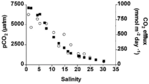
Figure 1 shows an example of pCO2and related flux values measured in the Scheldt estuary in July 1996. Both the pCO2and the efflux increase when salinity decreases. pCO2and dissolved oxygen profiles obtained in the Scheldt, the Thames, the Gironde, and the Rhine estuaries (Fig. 2) illustrate that the pCO2variation with salinity is quite different from one estuary to another, though the su-persaturation is always high. All four estuar-ies show a clear increase of pCO2within the upper estuary (low salinity), which is associ-ated with a decrease in oxygen saturation. This increase in pCO2 is located at the tur-bidity maximum, at a salinity of about 1 in both the Gironde and the Rhine estuary, and a salinity of 10 in the Thames estuary. The Scheldt is already heavily polluted in the freshwater members and, in November 1997, we carried out sampling in the upper estuary, in the tidal river, and in the tributaries (Fig.
Universite´ de Lie`ge, Me´canique des Fluides Ge´ophy-siques, Unite´ d’Oce´anographie Chimique, Institut de Physique (B5), B4000 Lie`ge, Belgium.
*To whom correspondence should be addressed. E-mail: [email protected]
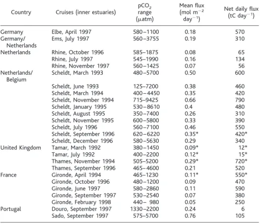
Table 1. Data collected during research cruises within inner estuaries. Before 1995, pCO2was calculated
from total alkalinity and pH measurements, the latter being calibrated using buffers proposed by the U.S. National Bureau of Standards. After 1995, a system coupling an equilibrator and an infrared gas analyzer (Li-Cor 6262, Li-Cor, Lincoln, Nebraska), was used for pCO2lower than 3500matm. Lower pCO2values
are from the river mouth (lower estuary, high salinity), whereas higher values are from the turbidity maxima (see also Fig. 1), usually located in the upper estuary (low salinity). Fluxes were measured in the field (28) or calculated (*) according to (27). The net daily flux is calculated over the entire surface of estuaries, and the mean flux is the corresponding averaged value per square meter.
Country Cruises (inner estuaries) pCOrange2 (matm)
Mean flux (mol m22
day21)
Net daily flux (tC day21)
Germany Elbe, April 1997 580–1100 0.18 570
Germany/ Ems, July 1997 560–3755 0.19 310
Netherlands
Netherlands Rhine, October 1996 585–1875 0.08 65
Rhine, July 1997 545–1990 0.16 134
Rhine, November 1997 560–1425 0.07 56 Netherlands/ Scheldt, March 1993 480–5700 0.50 600
Belgium Scheldt, June 1993 125–7200 0.38 460 Scheldt, March 1994 400–4450 0.35 420 Scheldt, November 1994 715–9425 0.66 790 Scheldt, January 1995 530–8610 0.4 480 Scheldt, August 1995 350–7400 0.26 310 Scheldt, November 1995 600–5800 0.33 390 Scheldt, July 1996 560–7100 0.46 550 Scheldt, September 1996 620–6220 0.35* 420* Scheldt, December 1996 580–5630 0.29 340 United Kingdom Tamar, March 1992 380–1450 0.09* 12*
Tamar, July 1992 400–2200 0.12* 15*
Thames, November 1994 505–5200 0.29* 720* Thames, September 1996 465–4600 0.21 520
France Gironde, April 1994 465–1230 0.11* 550*
Gironde, October 1996 480–1200 0.09 470
Gironde, June 1997 580–2860 0.11 590
Gironde, September 1997 530–2540 0.07 380 Gironde, February 1998 440– 980 0.05 250 Portugal Douro, September 1997 1330–2200 0.24 6 Sado, September 1997 575–5700 0.76 105
R
E P O R T S
16 OCTOBER 1998 VOL 282 SCIENCE www.sciencemag.org
434
3). The pCO2is quite high in the tributaries but increases drastically at the entrance of the estuary, together with a drop in particulate organic carbon (POC). The CO2distribution within estuaries is therefore the result of physical mixing of supersaturated freshwater with seawater, of marked heterotrophy in the upper estuary, and of CO2efflux to the atmo-sphere. Annual budget calculations have shown that 50% and.90% of the POC load transported into the Gironde (12) and the Scheldt (5), respectively, are mineralized in the turbidity maximum. In contrast, dissolved
organic carbon (DOC) is mostly refractory and behaves conservatively through estuaries (13). Table 1 shows that the highest pCO2 values at the turbidity maximum range from 1100matm in the Elbe estuary in April 1997 to 9500matm in the Scheldt estuary in No-vember 1994. For inner estuaries, where the total surface is known, corresponding net dai-ly fluxes to the atmosphere have been calcu-lated from discrete CO2flux measurements. Except for the small estuaries, CO2 fluxes amount to several hundred tons of C (tC), with a maximum of 790 tC day21in Novem-ber 1994 in the Scheldt estuary.
The POC mineralization produces 150 and 400 tC daily in the Gironde and the Scheldt estuaries, respectively. The flux val-ues given in Table 1 then suggest that, in the Scheldt, about two-thirds of the flux results from heterotrophy, with the remaining third resulting from physical ventilation. In the Gironde estuary, about one-third of the atmo-spheric flux is due to heterotrophy.
In polluted European estuaries, most of the labile carbon that is respired is anthropo-genic (4, 5). Other pollution-related process-es, such as nitrification in the Scheldt estuary (2, 14), may also acidify estuarine water and favor the CO2flux to the atmosphere.
These data show that the investigated in-ner estuaries are a CO2 source to the atmo-sphere, ranging from about 0.10 mol m–2 day–1to 0.76 mol m–2day–1. The estuarine area we studied emits 3000 tC daily to the atmosphere, corresponding to a mean flux of 0.17 mol m–2day–1.
Outer estuaries can differ substantially from inner estuaries as sources for atmo-spheric CO2. The outer estuary can be a site of intense primary production, because of eutrophication, and can behave as a sink for atmospheric CO2. The data in Table 1 show that significant undersaturation occurred in the lower Scheldt in June 1993, but that supersaturation was observed in all other cas-es. A time series of measurements, carried out over 18 months in the outer Scheldt es-tuary, shows that undersaturation only occurs for a few weeks during the spring phyto-planktonic bloom (15). Table 2 shows that supersaturation appears to be the general ten-dency in the outer estuary, and rates of efflux are about one order of magnitude lower than in the inner estuary (Table 1).
The above considerations have been used to
Fig. 1. Surface pCO2(in microatmospheres; full squares) and CO2 efflux (in millimoles per square meter per day; open circles) measured in the inner Scheldt estuary in July 1996 as a function of salinity. See legend of Table 1 for technical details.
Fig. 2. Distribution of pCO2(in microatmospheres; full squares, left axis) and dissolved oxygen (as percent saturation; open circles, right axis) as a function of salinity in the surface waters of some investigated inner estuaries.
Fig. 3. pCO2(solid bars, left axis) and particu-late organic carbon (as percent suspended par-ticulate material; open bars, right axis) in the upper Scheldt estuary (city of Antwerp), in the tidal river (35 km from Antwerp), and in some tributaries (60 km from Antwerp) in November 1997.
Fig. 4. Total carbon emission from European estuaries computed by taking into account the variability of the surface area for inner estuar-ies and the efflux from outer estuarestuar-ies. Based on our data, the efflux from inner estuaries was taken as 0.15 mol m–2day–1. Assuming that 20% of the European estuarine surface area are inner estuaries, with an efflux of 0.15 mol m–2 day–1, the outer estuarine influx should amount to –0.04 mol m–2day–1to yield a global null flux.
Table 2. Data collected during research cruises in outer estuaries. Low pCO2values correspond to high
salinity values. See legend to Table 1 for technical details.
Cruises (outer estuaries) Salinityrange pCO2range
(matm) (mol mMean flux22day21)
Elbe, April 1997 12–30 580–340 0.02 Ems, July 1997 30–34 560–525 0.03 Rhine, October 1996 25–34 585–385 0.02 Rhine, July 1997 18–33 545–375 0.015 Rhine, November 1997 25–31 560–430 0.015 Scheldt, July 1996 30–32 560–540 0.035 Scheldt, September 1996 30–34 620–450 0.03* Scheldt, December 1996 30–34 580–450 0.03 Scheldt, March 1997 30–34 580–240 0 Scheldt, August 1997 31–34 640–410 0.03* Gironde, September 1997 30–33 580–550 0.035 Douro, September 1997 9–30 1330–385 0.05 Sado, September 1997 32–34 575–450 0.03
R
E P O R T Sestimate total CO2 emission from European estuaries (Fig. 4), which appears to be a signif-icant percentage of the present anthropogenic CO2 release to the atmosphere from Western Europe due to combustion [647 million tons of C in 1995 (16)]. A minimum estimate, calcu-lated by applying an outer estuarine efflux of 0.01 mol m–2day–1to 80% of the total Euro-pean estuarine surface area, yields a total European emission of 20 million tons of C per day, representing 3% of the present anthropogenic emission of CO2from West-ern Europe. It is likely that the percentage of surface area of inner estuaries is in the range of 25 to 50% and, from data present-ed here, we estimate the actual value to be in the range of 30 to 60 million tons of C per day, which is 5 to 10% of the present European anthropogenic emission. This percentage has been obtained for a highly industrialized area of the world; it may be higher for developing countries, where an-thropogenic CO2 emissions are lower and where significant organic carbon load re-sults from overpopulation.
Few data are available for other estuaries in the world, but the available data shows a high degree of supersaturation (1, 17–19), ranging from 500 to 6000matm. Some data are also available for major rivers. The car-bon budget of the Amazon has been studied (20), and it was shown that this river emits 0.17 to 0.52 mol m–2
day–1
, very similar to our flux data. Carbon dioxide levels have been measured in the Niger (21), and the highest values reported were ;6400 matm, again in agreement with values reported here.
References and Notes
1. S. Kempe, Mitt. Geol.-Palaeontol. Inst. Univ.
Ham-burg 52, 719 (1982).
2. M. Frankignoulle, I. Bourge, R. Wollast, Limnol.
Oceanogr. 41, 365 (1996).
3. P. M. Woodwell, P. H. Rich, C. A. S. Hall, in Carbon and
the Biosphere, P. M. Woodwell and E. V. Pecan, Eds.
(U.S. National Technical Information Service, Spring-field, VA, 1973), pp. 221–240.
4. S. Kempe, J. Geophys. Res. 89, 4657 (1984). 5. R. Wollast, in Pollution of the North Sea, An
Assess-ment, W. Salonmons, B. L. Baynes, E. K. Duursma, U.
Fo¨rstner, Eds. (Springer-Verlag, Berlin, 1988), pp. 185–193.
6. S. V. Smith and J. T. Hollibaugh, Rev. Geophys. 31, 75 (1993).
7. J.-P. Gattuso, M. Frankignoulle, R. Wollast, Annu. Rev.
Ecol. Syst. 29, 405 (1998).
8. C. H. R. Heip et al., Oceanogr. Mar. Biol. Annu. Rev.
33, 1 (1995).
9. W. H. Schlesinger, Ed., Biogeochemistry: An Analysis
of Global Change (Academic Press, London, 1997).
10. S. Kempe, LOICZ Reports & Studies 1, 1 (1995). 11. S. V. Smith and J. T. Hollibaugh, Ecol. Monogr. 67,
509 (1997).
12. H. Etcheber, thesis, Universite´ de Bordeaux (1986). 13. R. F. C. Mantoura and E. M. S. Woodward, Geochim.
Cosmochim. Acta 47, 1293 (1983).
14. G. Billen, Estuarine Coastal Shelf Sci. 3, 79 (1975). 15. A. V. Borges and M. Frankignoulle, J. Mar. Syst., in
press.
16. G. Marland, T. A. Boden, A. Brenkert, R. J. Andres, J. G. J. Olivier, in Fifth International Carbon Dioxide
Conference, Cairns, Australia, 8 to 12 September
1997 (CSIRO, Aspendale, Australia, 1997), p 4.
17. P. K. Park, L. I. Gordon, S. W. Hager, M. C. Cissel,
Science 166, 867 (1969).
18. P. A. Raymond, N. F. Caraco, J. J. Cole, Estuaries 20, 381 (1996).
19. W.-J. Cai and Y. Wang, Limnol. Oceanogr. 43, 657 (1998).
20. J. E. Richey, R. L. Victoria, E. Salati, B. R. Forsberg, in
Biogeochemistry of Major World Rivers, E. T. Degens,
S. Kempe, E. Richey, Eds. ( Wiley, New York, 1991), pp. 57–74.
21. O. Martins and J.-L. Probst, in (20), pp. 127–155. 22. P. S. Liss and L. Merlivat, in The Role of Air-Sea
Exchange in Geochemical Cycling, P. Buat-Me´nard, Ed.
(NATO ASI Series, Reidel, Utrecht, Netherlands, 1986), pp. 113–128.
23. F. Jordan, F. Clark, R. Wanninkhof, P. Schlosser, H. James, Tellus B 46, 274 (1994).
24. R. Wanninkhof, J. Geophys. Res. 97, 7373 (1992). 25. J. P. Bennet and R. E. Rathbun, U.S. Geol. Surv. Prof.
Pap. 737 (1972).
26. M. Frankignoulle, Limnol. Oceanogr. 33, 313 (1988). 27. F5 K a DP, where F is the flux in mol m22s21, K is the exchange coefficient in m s21,a is the CO
2 solubility coefficient in mol m23atm21, andDP is the CO2gradient through the interface [pCO2(water)– pCO2(air)] in atmospheres. An exchange coefficient of 23 1025m s21(that is, 8 cm hour21) (2, 22, 23) was used for a Schmidt number Sc5 600 (24), which is a typical value for a moderately turbulent river (25).
28. Atmospheric exchanges of CO2were measured using
the direct floating chamber method (26) adapted for operation in estuarine environments (2). The chamber was set up on a lagrangian system in order to avoid creation of turbidity due to estuarine current and to follow the same water mass. Measurements were typ-ically carried out each 2.5 salinity step through the whole estuary. Wind speed is usually low in investigated areas (0 to 5 m s21), and the exchange coefficient K (27) is mainly determined by the turbulence of the water column. Calculated values of K, from measured flux and CO2gradient (27), is in good agreement with those reported for rivers (25). It should be pointed out that, if wind becomes predominant, actual efflux would be higher than our estimate.
29. We thank the crews and technicians who were in-volved in the numerous cruises, R. Wollast and two anonymous referees for helpful comments on a pre-vious version of this manuscript, and A. Pollentier, J. Backers, and A. Peliz for providing salinity and tem-perature data. Funded by the Fonds National de la Recherche Scientifique (FNRS, Belgium), with which the senior author is a research associate, and the European Union [Marine Science and Technology (MAST ) and Environment and Climate programs]. This is a contribution to the European Land Ocean Interactions Studies (ELOISE) Programme (publica-tion number 037) in the framework of the Biogas Transfer in Estuaries (BIOGEST ) project carried out under contract ENV4-CT96-0213.
23 June 1998; accepted 28 August 1998
A Short Circuit in Thermohaline
Circulation: A Cause for
Northern Hemisphere
Glaciation?
N. W. Driscoll and G. H. Haug
The cause of Northern Hemisphere glaciation about 3 million years ago remains uncertain. Closing the Panamanian Isthmus increased thermohaline circulation and enhanced moisture supply to high latitudes, but the accompanying heat would have inhibited ice growth. One possible solution is that enhanced mois-ture transported to Eurasia also enhanced freshwater delivery to the Arctic via Siberian rivers. Freshwater input to the Arctic would facilitate sea ice formation, increase the albedo, and isolate the high heat capacity of the ocean from the atmosphere. It would also act as a negative feedback on the efficiency of the “conveyor belt” heat pump.
Major ice sheet growth in Eurasia, Green-land, and North America is recorded by a d18O enrichment in benthic foraminifera between 3.1 and 2.5 million years ago (Ma) (1, 2) and by the massive appearance of ice-rafted debris in northern high-latitude oceans since 2.7 Ma (3). An increase in the d18O value of benthic foraminifera predom-inantly reflects the growth of continental ice volume. The intensification of Northern Hemisphere glaciation (NHG) finalizes the
Cenozoic cooling trend, which started in the early Eocene and is marked by the first indications of ice sheets in Antarctica 36 Ma (4). This long-term cooling brought the climate system of Earth to a state critical for ice sheet buildup in the Northern Hemi-sphere. This has been the case since ap-proximately 11 Ma, when the first and mi-nor occurrence of ice-rafted debris in the Arctic and North Atlantic indicates the first attempts of the climate system to start a glaciation (5). However, the climate system failed to generate and maintain major ice sheets in the Northern Hemisphere until 2.7 Ma. Here we suggest that the closure of the Isthmus of Panama, which enhanced mois-ture transport to the Eurasian continent, N. W. Driscoll, Woods Hole Oceanographic
Institu-tion, Woods Hole, MA 02543, USA. G. H. Haug, GEO-MAR, Forschungszentrum fu¨r Marine Geowissen-schaften, Universita¨t Kiel, Wischhofstrasse 1–3, D–24148 Kiel, Germany.
R
E P O R T S16 OCTOBER 1998 VOL 282 SCIENCE www.sciencemag.org