Methods for multi-class segmentation of molecular sequences

(1)

Methods for multi-class segmentation of molecular

sequences

par

Ming-Te Cheng

Département diiiformatique et de recherche opéra tioimelle Faculté des arts et des scieuces

I\Ïémoire présenté à. la Faculté des études supérieures Cil vue de Fobtention du grade de

Maître ès sciences (M.$c.) en informatique mars. 2006

Université de MontréaÏ

n

(2)

(3)

Université

dI

de Montréal

Direction des bibliothèques

AVIS

L’auteur a autorisé l’Université de Montréal à reproduire et diffuser, en totalité

ou en partie, par quelque moyen que ce soit et sur quelque support que ce soit, et exclusivement à des fins non lucratives d’enseignement et de recherche, des copies de ce mémoire ou de cette thèse.

L’auteur et les coauteurs le cas échéant conservent la propriété du droit d’auteur et des droits moraux qui protègent ce document. Ni la thèse ou le mémoire, ni des extraits substantiels de ce document, ne doivent être imprimés ou autrement reproduits sans l’autorisation de l’auteur.

Afin de se conformer à la Loi canadienne sur la protection des

renseignements personnels, quelques formulaires secondaires, coordonnées ou signatures intégrées au texte ont pu être enlevés de ce document. Bien que cela ait pu affecter la pagination, il n’y s aucun contenu manquant.

NOTICE

The author of this thesis or dissertation has granted a nonexclusive Iicense allowing Université de Montréal to reproduce and publish the document, in part or in whole, and in any format, solely for noncommercial educational and research purposes.

The author and co-authors if applicable tetain copyright ownership and moral rights in this document. Neither the whole thesis or dissertation, nor substantial extracts from it, may be printed or otherwise reproduced without the author’s permission.

In comptiance with the Canadian Privacy Act some supporting forms, contact information or signatures may have been removed from the document. While this may affect the document page count, it does flot represent any loss of content from the document.

(4)

Ce mémoire intitulé

Methods for miilti-class segmeutation of molecular seqiieuces

présenté par

Miug-Te Cheng

a été évalué par un jury- composé des personnes suivantes:

François Major président—rapporteur MikÏés Cstfrés directeur de recherche $ylvie Hamel membre du jury

(5)

Résumé

Le mémoire présente les modèles statistiques pour la segmentation de séquelices

moléculaires. Il décrit des algorithmes de segmentation et leur implémentation. en utilisant diverses méthodes de pénalisation pour la complexité du modèle. avec des restrictions possibles des longueurs de segments. Les méthodes sont illustrées sur

les séquences JADN du bactériophage lambda, Methanocaïdococcus jannaschiz. et du complexe majeur dliistocompatibilité huniain.

(6)

The thesis discisses statist.ieal moclels for the segme1tatioll ofmoleciilar sequences. It describes segmentation algorithms and tiieir impÏementation. using varions penal izatioli methods for model complexity, along with possible restrictions on segmelit lengths. The methocis are illnstrated 011 the DNA seciueiices of bacteriophage lambda,

Mcthanocaldococcus jannaschii and the human Major Hstocompatibi1ity Complex.

(7)

fl

5.2 RNA Genes in Thermophules 71

5.2.1 Description 71

5.2.2 Tests 74

5.2.3 Resuits 71

5.3 Major I-Iistocompatibilitv Complex 93

5.3.1 Description 93 5.3.2 Tests 93 5.3.3 Resuits 95 6 Conclusions 98 6.1 Discussion 9$ 6.2 Future Work 99 11

n

(9)

List of Figures

2.1 I\ioledlllar structure of the 2’-deoxyribose suga; 5

2.2 $chematic molecula; view of a DNA strand 5

2.3 Molecular structure of nucleotide bases with hydrogen bonding 6

2.4 Schematic molecular view of a double strand of DNA 7

2.5 Reciprocal and non-reciprocal recombination following crossing-over li

3.1 An example of HMM modelling isochores in human genome 24

1.1 Illustration of operations reciuired for computing forward variable 29

4.2 Illustration of comput ing forward variable in terms of observations and

states 30

1.3 Illustration of operations required for computmg backwarcl variable. 32

4.1 Penalty—based best segmentation algorithm 37

4.5 Penalty—basecl best segmentation with traceback arra algorithm 38

4.6 Traceback aigorit hm 4t)

4.7 I\Iaximmn-likelihood estimation of segments algorithm 40

4.8 Penalty-based minimum leiigth segmentation algorithm 44

4.9 Penalty—basecl minimum length segmentation with traceback array al—

gorithm 46

(10)

5.1 Probabilitv calculation algorithm 51

5.2 Add data to traceback airay algorithni 52

5.3 Byte compression i;ito t.raceback array algorithm 53

5.4 Read data to traceback array algorithm 54

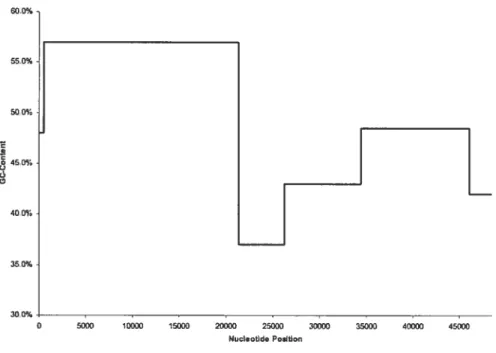
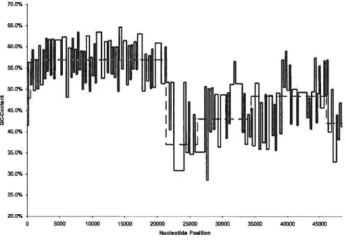
5.5 Byte decompression from traceback arrav aÏgorithm 55 5.6 Distribution iII bacteriophage /\ via gradient centrifugation .56

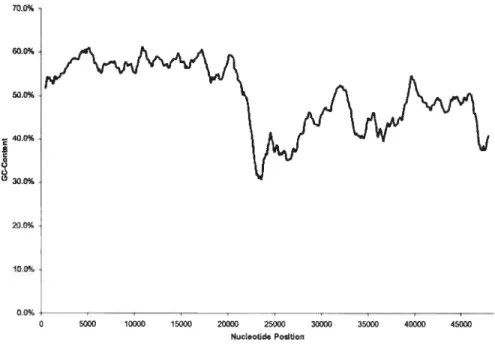
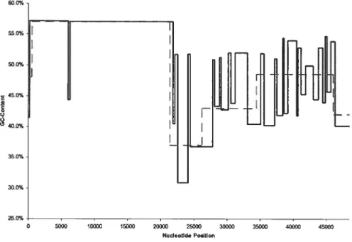
5.7 Distribution in bacteriophage \ via EMBO$S 57

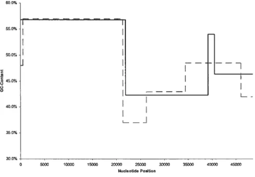
.5.$ Bacteriophage À comparison (2 classes. BIC and MDL) 60

5.9 Bacteriophage À with miniiinim lengths coniparison (2 classes, none) 62

5.10 Bacteriophage ,\ with minimum lengths comparison (2 classes. AIC) 63

5.11 Bacteriophage À with minimum lengths comparison (3 classes. none) 65 5.12 Bacteriophage À with minimum lengths coniparison (3 classes .AIC) 66

5.13 Bacteriophage À comparison (1 classes, BIC) 69

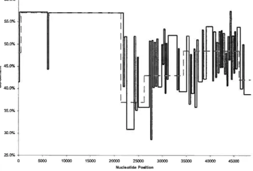
5.14 Bacteriophage À versus EMBOS$ distribution (4 (lasses. BIC) 7t)

5.1.5 G C-content of RNase P RNA genes in Prokarotes versus optimal

growth temperatnre 72

5.16 Helical GC-content of RNase P RA genes in Prokar otes versus op

timal growth temperature 73

5.17 M. jann.ascÏih comparison (2 classes. BIC cmd MDL) 7$ 5.18 M. jaîznascÏLii comparison (3 classes, BIC aid MDL) $2

5.19 IIL jannaschi:i with minimuni lengths comparison (3 classes. BIC anci

MDL) $3

5.20 M. jannaschii comparison (6 classes. BIC and MDL) $5

(11)

n

5.21 M. jannaschii with minimum lengths comparison (6 classes, BIC and

MDL) 86

5.22 M. janr?achi comparison (10 classes, BIC aid MDL) 90

5.23 M. /anriascÏiii with minimum le;igtlis coniparison (10 classes, BIC and

MD1) 91

5.24 Segmented MHC sequence 94

5.25 MHC cOmpalison (4 classes, BIC auJ MDL) 95

5.26 MHC with mininmm lengths comparison (4 classes. BIC and MDL). 96

5.27 MHC with minimum leiigths versus EMBOSS distribution (4 classes.

BIC) 97

(12)

5.1 Bacteriophage À via densitv centrifugation quantitative data 56

5.2 Complexity penalty values n tested for bacteriophage À 58

5.3 Prohability values pj(.T) t.ested for bacteriophage À 58

5.4 Minimum length values testeci for bacteriophage À 59

5.5 Distribution in bacteriophage À for BIC and MDL tests (2 classes) 61

.5.6 Bacteriophage À comparison (2 classes. BIC auJ MDL) 61

5.7 Bacteniopliage À expenimental data (2 classes) 61

5.8 Bacteriophage À with minimum lellgths companison (2 classes, none) 62

5.9 Bacteniophage À witÏi minimuni Ïengtlis comparison (2 classes. AIC) 63

5.10 Bact.eriophage À witli minimum lengths experinental data (2 classes) 61

5.11 Bacteriophage À with minimum lengths comparisou (3 classes. BIC

and MDL) 65

5.12 Bacteriophage À witli minimum lengths comparison (3 classes. noue) 66

5.13 Bacteriophage À with minimum lengths comparisou (3 classes. AIC) 67

5.14 Bacteriophage À experimeHtal data (3 classes) 67

5.15 Bacteniophage À with minimum leugths experiniental data (3 classes) 67

5.16 Bacteriophage À witii nuiuiinum lengths conuparisoil (4 classes, BIC). 68

5.17 Complexity peuafty values o testecl foi’ iL jannaschii 74 5.18 Probability values pj(X) tested for M. jaflflC$CÏuz? 75

(13)

5.19 Minimum length values tested for iiI. jartnaschii. . 76

5.20 RNA fonnd for M. annaschu (2 classes) 79

5.21 Experimental data for M. ]ann ascÏin (2 classes) 80

5.22 RNA founcl f& M. janraschn (3 classes) 81

5.23 Experimeutal data for iiL jannuscÏnz (3 classes) $1

5.24 RNA fourni fbr M. jaunascim (6 (lasses) $7

.525 Experimental data for M. janriuscÏiii (6 classes) . . 88

5.26 RNA fourni for M. jannaschii (10 classes) $9

5.27 Experimeutal data for M. .iann aschi (10 classes) 92

5.28 Complexity penalty values a tested for MHC 93

5.29 Probability values pj(:r) tested for MHC 94

5.30 Minimum leigth values tested for MHC 94

(14)

viii

n

(15)

Acknowledgment

s

I woiild like to thaiik Di. Iik1és Csfirs for his invahiable friendship. inspiration,

snpport, patience. and guidance. which were crucial in bringing this thesis in finition. I would like to thank my friends for their encouragement in completing this thesis. finally, I would like to tliank mv parents and my brother for their prayers, cri

couragement, and love.

(16)

Introduction

La.rge-scale seqiiencing lJrojects like the Hiinian Genome Project prochice a great wealth and variety of seqilelice data. Molecrilar sequeiices in sequence data banks such as GenBank of the National Center of Bioteclmology Information (NCBI) adcl up to more than 100 billion base pairs now. There is an increasing need of developing

efficient tools to analvze these sequences. A class of analysis methocls involves se— qneirce segmentation. consisting of dividhiig a sequence into fahJy homogeneoris paits by some measure of homogeueity.

Csuirs (2004) investigated the problem of determiuing maximum-scoring segment

sets that can be applied to a nnmber of molecular biology problems. such as DNA and

protein segmentation. To calculate poteutial segment sets for a given seqnellce, Csûrs presented a nuiiiber of fast algorithms in which differeirt statistical models were used

for two classes. In ouï research work, we clemonstrate how sequence segmentation

(17)

9

1.1 Plan

In Cirapter 2, we provide a brief introduction to DNA auJ isochores. We also give

a description of the proposais that eventually lcd to tire existence of the isochore

theory. Furthermore, we prescrit arguments pertaining to the actiial existence of

isochores. In addition to problems associated with the seqence segmentation baseci on isochore content, we disdllss diffèrent applications of segmentation algorithms to other problems.

I1Î Chapter 3, we present statistical modeis that can lie rised in segmentation. inciriding Bayesian and hidden Maikov model, as well as statistical notions of coni plexity.

In Chapter 4, we prescrit the aigorithms that can lie used to soive tire probleins encountereci in segmentation statistical modeis. We aiso present tire penaÏty-based best segmentation model. First, we provicle a description of how this modei eau lie

impiemented throngh dynamic prograruming. $econdiy. we prescrit tire impiemented

aigorithins without anci with traceback. Thirdiy, we show how tins modei cari lie

iucorporated in maximum-likelihood estimation. Finaliy. we clemonstrate how mini— mnnr segment iength values can lie incorporated into tins modei.

In Cirapter 5, we present tire experiments rised to evainate onr implemented ai

gorithms on three sequences: bacteriophage- genonie. tire genome of Methanocaldo

cocc’us jannaschii (M. jannaschii), and tire seqiience of the major histocompatibiiity

compiex (I\1HC) oir human chromosome 6. We prescrit the tests nsed for eacir se

quence auJ tire observed resuits.

Chapter 6 provides a snmmary of tire discnssed segmentation concepts auJ. most

(18)

1.2 Contributions

To carry otit our sequence segmentations. we extenci the two-class algorithms pre sented by Csiirds (2004) to propose two algorithnnc models that uses an arbitrary number of classes: the penalty—based best segmentation model ancl the penalt-based best segmentationwith minimum segment lengths model. Aithougir both moclels par tition a given sequence using maximum-likelihood estimation, only the latter takes

minimum segment lengths info consideration. We also incorporated the best segmen

tation score for the implementeci traceback algorithms to refer to when determining

the best segmentation of a sequence. For model parameter estimation. we proposed the use of Laplace pseudo-counters. As weÏL we incorporated the data compression algorithm in order to reduce the amount of allocated memory. We implemented ouï

segmentation models using Java and evaluated flic clifferent penalization methods

on bacteriophage-À. M. jannascÏiii, and MHC on liuman chromosome 6. Finally, we

conclucted a RNase P analysis of heilcal and non-helical GC-content versus optimal growth temperat ure on Prokaryotes.

(19)

Chapter 2 Segmentation in $equence Analysis

2.1 DNA: A Brief Introduction

Deoxyribonucleic Acid (DNA) is a rnicleic acid that contains the genetic information

required for aniy orgauism to functioll biologically (Watson auJ Crick 1953). As

initiaïly proposed by James Watson and Francis Crick in 1953, it is charactenized as a double helix where cadi uucleotide base in one strand is boncled to a base in the other strand.

Each strand is a chain of repetitive units known as nucleoticles. A nucleotide consists of a 2’-deoxyribose sugar auJ a phosphate group with a so-called base. Tic molecular structure of tic sugar is ihlustrated in Figure 2.1, where the numberecl values represent carbon atom positions. DNA is measurecï in base pairs, tliat is, kbp (thousand base pairs). Mbp (million base pairs). auJ Gbp (billion base pairs) are “units’ used in tlie Biotechnologv community.

As shown in Figure 2.2. nucleotides eau form a polynucleotide chain by connectmg to each other through a covalent bond between tic 3’-carbon of one nucleotide. the

phosphate residue. auJ tic 5-carbon of tic next unit. The sugar auJ phosphate

molecules are represented as ‘r auJ •p” svmbols. respectively.

(20)

H HO---U 3i 2’ flO H base

Figure 2.1. Molecular structure of the 2’-deoxyribose sugar (Setubal and Mei danis 1997).

Figure 2.2. Schernatic molecular view of a DNA strand (Setubal and Meidanis 1997).

(21)

6

DNA molecules iormally comprise two polyiiucleoticles. called strands. Each 1’-carbon in the strand contains a nucleotide base attacheci to it. which eau be one of the four different types: adenine (A). gnaule (G). cytosirie (C). and thymine (T). Nucleotide bases caribe categorizeci into two maili groups, namely. purines (A and G) and pyrimidines (C and T). The strands are connected togetiier by forming hydrogen bonds at the bases as illustra.ted in figure 2.3, where A-T auJ C-G are clefined as complementary or Wat son-Crick base pairs. Figure 2.4 provicles a schematic molec niai structure view of a double strand of DNA. A DNA molecule is determined tims by the sequence of bases ou one of its strands. representeci as a sequence of characters over the alphabet {A. C, G. T}.

H /C% ____ Sugar N Guanine C C,, / / N.

/

H N H _N H /‘ .0 C Cytosine

I

NC Suar H

Figure 2.3. Molecular structure of nucleotide bases with hydrogen bonding (dot ted unes) (Setubal and Meidanis 1997).

H Sugar— _N(> Adeninel H

/

\

f

N _,C

b

\

_4,

N—C. /1 _____ C—CH3 /1 Thynirne

\,

/NC\ Sugar H

(22)

Figure 2.4. Schematic molecular view of a double strand of DNA (Setubal and Meidanis 1997).

2.2 Isochores

Sequence segmentation involves dividing a giveil sequeilce into fairlv liomogeiieous

parts by some measure of homogeneity. As an example. we cliscniss lieue the segmeil

tatimi of a DNA sequence into so-called isochores.

2.2.1 Description

A inofile of gnianine auJ cvtosine (GC) levels eau Le used to characterize variation along chromosomes. where the natural partition of a chromosome sequence is clefined

as ahrnipt changes iii GC level (Paces et al. 2004). GC levels are correlated with key lilological properties in mally eukarvotes. sucli as geiie dellsity changes. replication

timing switches. auJ dlifferences Letween the locations of acljacellt regiolls in the mterphase nucleils.

(23)

$

position of the genomes of waim-blooded vertebrates. Unlike the classical work of

Meselson et al. (1957) where CsC1 densitv gradients were useci iii equilbrium cent.rifu— gation to reveal broaci, assvnietricai bands in DNA. Filipski et aÏ. (1973) proposed that high-resolution fractionation is possible by using eciuilibriuin centrifugation in

C52SO4_Ag+

density gradients instead to partition DNA-silver complexes according

to the frequency of silver-binding sites on DNA molecules. When applied to bovine

DNA, this technique revealed three distinct fainilies of fragments (coinprising 85 of the genome) havillg different GC content. This subsequently led to the discovery that DNA fractionation reveals the compositiollal heterogeneity of high molecular weight. “main band” (i.e. non-satellite. non-ribosomal) bovine UNA. Purthermore, the lab—

orator conchideci that vertebrate genomes are comprised of a mosaic of isochores,

which are defineci as long DNA segments of more than 300-kbp that are composition

ally honïogeneous ancl belong to a smai number of families dharacterized by different GC levels.

These isochores reftect a level of gellome organizat ion (Eyre-Waiker auJ Hurst

2001) since it is observed that GC-rich components of the genome yielded a higher

number in terms of gene density. short interspersed repetitive DNA elements, anci

recombination frequencv. For GC-poor components of the gellome liowever. it is

founcl that they ahnost exclusively possess long interspersecl repetitive DNA elements.

2.2.2 Proposed Causes

Scientists are interested in finding an explanation of why there is a large-scale varia

tion in base composition aÏong chromosomes. It was snggested that variation could

be due to three noll-mutuallv exclusive processes: mutation bias. natural selection.

(24)

Mutation Bias

Different base composition cari be expected if there are clifferent mutation processes acting on different parts of the genome. With a simple probabilistic moclel. assume that each nucleotide may mntate independentiv by

tue

same mutation probabilities along the sequence. The base composition wiil converge towards the stationary prob

ahilities determined by the substitution probabilities. If the mutation probalilities are not iclentical along tire genome. then tire base compositioir wiii vary too.

Wolfe et al. (1989) noted that tire concentrations of free nucleotides affect tire

pattern of base misincorporation cluring DNA replication. For exampie. G and C

nucleotides tend to be preferelÎtialiy misincorporated hrto DNA tirat is rephcated in

a pool of free nticleotides rich in G and C. They also observed that free nucieotide

coircentrations vary duriirg the ccii cycle. and that different parts of tire genome

are repïicated at different thrres. Woife et al. coircirideci that tire regions of the

genonre with different rephcation times shonïd have different mntatioir patterns. and. ultimateiy. different base compositions.

Fihpski (198f) hvpothesized tirat variation hr tire efficiency of DNA repair niight

be responsibie fbr the formation and maintenance of isochores. He reasoned that tins

is due to tire variable cfficiencv of certain types of DNA repair aird that some types ofpair are known to he biased. therehv cansing variation hi tire pattern of nrutation.

Fryxeli and Zuckerkandï (2000) snggesteci tirat isochores are a consecience of

cytosine deanrination. which is defined as the reaction of a water moiecuie with tire

anrino group on position 4 of the pyriniidine ring of cytosine. thereby resniting in tire conversion of cvtosine to uracii (Eyre-Waiker aird Hurst 2001). They found that the

deaniination of nretlryi-cytosine and cytosine (i.e. C to T and C to U. respectively)

is expected to occur more easiiv in AT-rich DNA than in GC-rich DA since tire fornier tends to be more nirstabie. Tirev proposeci tirat an isochore structure cair

(25)

10

a rechiction in cytosme deamina.tion and an increase in GC content in the surrorind are as.

Natural Selectioir

Bernarcli and Bemnardi (1986) suggested that isochores are the cousequence of natumal selection. which is defined as the differeutial multiplication of mutant types. This oc— cuis through either negatwe selection. that is. the elimination of orgaiisms with dde—

tenons mutations. or positive selection via tl1e preferential pmopogation of omganisms

with advantageous mutations with respect to environmental pressures. One hypoth—

esis implies that natural selection acts upon the increased thermostabihty of DNA caused by GC-enrichnieut in orcler t.o aciapt to ally ten;pemature incmease in warni—

blooded ventebrates. wheme theme is a teudency for GC-nich DNA to be more thermally

stable than AT-rich DNA. To clemonstrate tins hypothesis. Bernardi neferred to Hie isochores found in the human genome. where the GC-ricliest and gene-ricliest iso choies found in a set of R(everse)-chromosomal bauds coincide with the T(elomenic) chromosomal bauds previously identified as part iculari resistant to thermal denat—

uration (Saccone et al. 1993). As well. a difference in amino-acid compositions and hydropathies bctween GC-rich auJ GC-poor isochores was observed.

Unlike the observations made for warm-blooded vertebrates. previous work con cluded that there was no comrelation betweeu GC—content and habitat temperature

hi Hie case of prokaryotes (Galtier and Lobrv 1997; Hurst ancl Mercliant 2001) ancï coïci-bloodeci vertebrates (Belle et al. 2002: Ream et al. 2003). furtiiermore. Vino

graclov (2001) observed that the benclability of genomic seciuences of warm-blooded vertebrates increased faster than their themniostability as the GC-content increased. 1-leuce, Vinogradov (2003) proposecl an alternative hvpothesis in which the formation

of isochores was pnimarily due to the beudabilitv. and not thermostability. of the UNA niolecule for active transcription in the GC-nich regions and for gene suppression in the GC-poor regions.

(26)

Ï’ A B C D A B C D A- B- C- D k B- C D A B C D k B- C D A B C D Crossinq ovt I k B- C- D

I

Reciprocal recombinenls A B C D — t I I A B’ C D

I

A B C- D I I k 8 C D

I

Non-eciprocaI recornb:nants

Figure 2.5. Reciprocal and non-reciprocal recombination following crossing-over (Watson 2004).

Biased Gene Conversion

Geire conversion is defineci as a non-reciprocal recombinatiori process that causes one

sequence to Le converted into file other. An illustration of a crossmg-over betweeri two dhromaticis (double-strancied DNA niolecules) is shown in Figure 2.5. We ciefine an alÏele as an alter-native form of a gene tirat occupies a specific position on a chromosome. Suppose that tire strancis contain a nmnber of alleles as indicated Lv aiphabetical letters. When cr-ossh;g-over occurs. there are two possible recombinants: reciprocal, where an equal 2:2 segregatioli of the entering alleles is observed: non

reciprocaL where o 3:1 segregatiori auJ gene conversion of allele B to B is exlïihited.

Crcnsinp oser and pane conversion

(27)

12

Biased gene conversion is when the two possible directions occnr with llnequal

probabilities (Eyre-Walker aiid Hmst 2001). Biased gene conversion woiild lead to a

base mismatch if the heteroduplex DNA extends across a heterozygous site. These

base mismatches are sometimes repaired bv the DINA-repa.ir machinery, although

they tend to be biased and thereby leading to an excess of one allele (i.e. one of the clifferent fonns of a gene or DNA seciuence that can exist at asingle locus) in reprocluctive ceils. Tiieir hvpothesis is baseci on two observations that clemonstrates the conrelation between the recombination rate and GC content. tliat is,

1. There is a correlation betweeii the frequencv of recombination and GC content

both between auJ within hunian chromosomes.

2. Sequences that have stopped recombinhig are either cledlinirig in GC content.

or have a lower GC content than their recombining paralogues (i.e. a locus that is homologous to another in the saine genome).

2.2.3 Existence

Demonstrated by the nunierous amount of studies silice its ftrst proposition, the isochore theory is considered to be the most reliable method of studying the long-range coinpositional structures of met azoan genomes witlnn an evolutionary frainework (Cohen et al. 2005). Purthermore. it is generallv assumeci that isochores exist and

tlïat they contain genes with corresponcling GC contents. When the draft of the hmnan genome was first proposeci, liowever. sonie scientists questioneci about the existence of isochores or at least tlieir usefulness.

The authors of the initial draft of the human genonle studied the gdllome sequence to examine whether strict isochores coulci be identified (Lancier et al. 2001). Tue authors clefined the terni “strict isochores as sequences that cannot be distinguisiieci

(28)

their argnmellt filaI isochores do not ment the prefix “iso”. Lander et al. divideci the human genome sequence into 300-kbp windows anci snbclivicleci each window info

20-kbp snbwindows. From calcnlating the average GC coiitent of each window and

snbwindow, and frorn exannning file relationsliip between the variance of the GC content in the subwindows and the avenage GC content in each window. Lander et al. concluded tliat

tue

idea of isochores Seing stnicti homogeneons can 5e rnled ont since the residnal variance was too large f0 Se consistent with a homogenons distribution. Despite the arguments of Lancier et ai., Li et al. (2003) maintained filaI isochores do ment the prefix “iso” . Li et al. presented two points in which the strict isochores

correspond to the isociiore concept originally developed and cleflned by Bernarcli. first, Bernardi (2001) defined isochores asfairtyhomogeneons regions. Unlike Lancier et aï.. Li et al. considered the GC mean vaines and val iance to Se two independent paiameters of a statistical distribution, and fomid support for flic isochore theory hi

the human genome sequence.

Cohen et al. (2005) examined whether if is possible to provide a concrete definition

of isochores so tiiat flic hnman genome can 5e descnibed as isochoric. They also

stnched file extent f0 winch each isochore can Se classified info a particular isochore

family. Their work n-as based on a number of cniteria tha.t they have proposed to describe the properties of isochores. namely:

1. C7iaractenistic GC content :An isochore is a DNA segment possessing a char

acteristic GC content tuaI significantly differs to tiiose in adjacent regions.

2. Hornogeneity : An isochore is more homogeneous in its composition than flic

chromosome on winch if resides.

3. Minimum. segment leugUi : The lengf h of an isochore typicaily exceecls 300-kbp.

4. Genonie coveruge : The overwhelniing majonity of the hnman genome consists of segments satisfying flic first three criteria.

(29)

14

5. Isochore farriilies The human genome is cornposed of five isodhore familles.

cadi with different Gaussian-clistributed GC content.

6. Isochore ass?gnmcmt into famities : Eadh isodhore can be associatecl with a

isochore familv based olll On its compositional properties.

To identify auJ quantify isocioric regions, Coien et ai. iised a binaiy redursive segmentation procedme proposeci by Bernaola-Galviin et al. (1996) to partition tic

human genome. Tic method repeatedly spiits the sequence based on an entropy

measure to maximize tic difference between neigiboming regions. A statistical test.

similar to tic one of Li et al. (2003) was used. The segmentation procedure revealed

tiat the distribution of segment lengtis does not have a ciaracteristic lengti scale. Coien et al. (2005) observed isodhores span less tian lïalf of flic sequenced portion of flic human genome if tiey satisfy tic first tiree attributes. but found tiat alternative isodhores with lower cutoif lengtis also satisfy fie same criteria. Altiougli flic iunïan

genome is traditionally clescribed ilsing five isociore families. Coien et al. fomid tiiat

four families aÏready capture tic GC content distribution. Pinally, Coien et al.

qiiestioned tic use of tic Gaussian model to define isodhores since tiey dicl not mcl

any evidence of a robnst multi-Ganssian description of alternative sets of isodhores.

Due to overlaps founci between candidate families, tiey also haci difficuit in reliablv classifying tic segments info families by compositional properties.

Althongi tic existence of isodhores rema.ins debatable up to

tus

point, ail studies

agreed tliat tic definition of isociores is relative. fiirtiermore. tiey agreecl tiat tic

genome does contain large iomogeneous regions of distinctive GC content. and is

worthwliile to redefine fie isochore concept to describe tic dvnaniics of GC content

(30)

2.3 Other Applications of Segmentation Models

In addition to isochores in higlier vertebrates, there is a wide variety ofsegmentation models which are used to answer a nnmber of biological problems. For instance, genome alignments exhibit a mosaic structnre where segments correspond to regions

with dlifferellt evoÏntionary pressrire.

Horizontal gene transfer between bacteria.. as demonstrated in a wide variety of ecosystems, plays an important 101e in the acquisition of aclaptive traits. such as pathogenicity. resistance to antibiotics or heavy metals like mercury and arsenic. furthermore, it is considereci to be lieavily influential in bacterial evolution. Bacteria are known to integrate prophages and have other ways of iritegrating foreign DNA se

quencestlirough DNA segments. Nicolas et al. (2002) used a statistical segmentation based approach to study heterogeneities in flic BacitÏ’us subtilis. $pecffically, they applieci hiclclen I\Iarkov moclels in which cadi type of segment is characterizeci by ifs

own statistical oligonucÏeotide compositioli. Their objectives were fo reconstruct seg

ments from DNA sequenccs arid dliaracterize tic identified segment types. with the aim of investigating correlations between segment types ancl biological DNA features

sucli as horizontal gene transfers. From their analysis. they revealed a number of

heterogeneities including those related to horizontal gene transfer, tic GT ricliness

of hvdrophobic proteins. and flic codon usage frequency of liighlv expressed geiles. The application of segmentation moclels f0 biological problems is not exclusive to

DNA sequence analysis. Romero et al. (1997) proposed metliods that predict locally clisordered (so-caled low complexity) regions that are based on physiochemical fea turcs of a set of relatively short clomains founcl in proteins of an otherwise kiiown

structure. Wootton and Federiien (1993) introduced tic SEC algorithm which auto—

matically partitions protein sequences int.o low— and high— complexity segments. Functional regions in genomic sequerices were traditionally predicted by identifv ig features associated with genes or regulatory regions. Functional regions tend to

(31)

16

be conserved in sequences that have evolved from a common ancestor. In contrast, non-functional regions are more likely to mutate. Consequently, functional regions can be

identifled in genomes using sequence

comparison. Non-functional

regions need

to be statistically diverged so that statistical procedures

can distinguish them from functional regions.

Because

of

this,

features present only at

dose

evolution&y prox imity are bat, thereby

limiting

the usefu]ness of such

comparisons

(McAuliffe et al.

2004). Boffeffi

et al. (2003)

used phylogenetic shadowing which involves segmenting

alipments

between

cbosely

related species

into

regions with high- and

bow- mutation rates. This

technique would enable the

bocalization of

regions

of

collective

varia tion

and complementary regions

of conservation, thus

facilitating

the identification of coding

and

non-coding

functional genes. Using

the phybogenetic shadowing

concept,

McAuliffe et ai

proposed

the generalized ffidden

Markov

phybogeny (GHMP) in

order

to

determine

the genomic sequences systematicafly, where the GHMP is presented as

a directed graphical modal (Jordan and

Sejnowski 2001).

Segmentation models can

also be

implemented

to partition

proteins into

a

number

of segments. Krogh et al. (1994) applied

hidden

Markov models W the problems

assodated

with statistical modeffing, database searching. ami multiple

alipment

of proteinfamilles

and protein

domain _{To construct their hidden Markov model, they}

defined

the 20 amino

_{acids from which}

protein molecubes are

composed

of as

states

and the strings of amino

acids that

form the

primary protein sequence as observations.

For eaeh set of proteins. their model

represents one

in

which

high probabffity to the

sequences

in that

particular set are assigned.

A

models

to

protein

partitioning is the tapol ou prediction of helical transmembrane proteins. Tusn4dy

and

Simon (1998) pro

posed

the HMMTOP method,

which is based

on the hypothesis

that

the

difference

in the amino acid distributions in

various

structural parts of these proteins determine the bocalizations of the

transmembrane segments and

the topobou. They constncted a

hidden Markov

model that

consisted

of

five states

that describe transmembrane

(32)

l)fotein structure: illsicle loop. inside lieux tau, membrane lieux. outsicle lieux tau.

and outside loop. Rather than accounting only the absolute amino acid compositions

ofvarions structural parts. tiïeir approach involves finding the combination of states that vield maximal divergences in the amino acid distribution. Alternatively. Krogh et al. (2001) presented file TMHMM method in whicli they take the alternation

between cytoplasmic anci noil—cytoplasmic loops in helical transmembrane proteins

into consideratioin Their hidclen Markov model consisted of seven types of states:

helix core, lieux caps on either side of the membrane. short ioop on cvtoplasmic side, short anci long loop on non-cytoplasmic side, and a globulai clomain state. Eacli

state contains a probability distribution over the 20 amino acids that characterizes

the variability of amino acids in the region it models. The a.mino acid and transition probabilities were calculated froni techniques that compute the maximum posterior

probabilities given a prior anci the observed freciuencies. The Ti\IHI\i I method pue dicts the transmembrane helices by cletermining the most probable t.opoÏogy given the hiciden Markov model.

(33)

Chapter 3 $tatistical Models

The acivautage of probalilistic models is that they cari ciescribe the relatioriships betweeu varions quaritities whule cousiderung the underiving uuicertainty associated with them. This leads to tire efficient use of a.vailaile information when making pre dictioris about biological sequences (Liii and Lawrence 1999). $tatistics is maunly

focused on makung inferences, which cari be defineci as tire process of deriving con clusions from facts ancl premises. lu our case. tire facts are the observeci data,

tue

premises are represented by a probabilistic model of biological sequences. auJ tire con clusions are relateci to the nmobserved quantities. This dhapter provides a description of a. number of statistical models that cari be usecl to segment a given molecular sequence.

Let be a fuite alphabet: for DNA sequences. Z = {A. C. G, T}. We consider

a. DNA sequence x r1r2 as tire observed value of a secuuence of random

variables X = X1X9 ... X. We define segments as a continuous unterval [i.

j]

such

tirat z . . . z5. Tire distribution of X is det.erminedbva seciuence of hidden

variables z = Z1Z. . . Z whiclr define these segments, where z {O k — 1}. Tire

segmentation vector. z is tire value taken by a rairdom variable Z Z1Z2 ... Z,.

(34)

P {X = ₌

j}.

Notice that we assume that these distributions do riot

clepend on

for a giveil segl;ÎciÏtation, the likeliliood of the observed sequerice is writtell as

L(z)=P{X=xZ=z}. (3.1)

The mai11 objective of usillg statistical models is to detennirie z. Equatioll 3.1 cari be expauded as

L(z) = flp(i. (3.2)

The log-likelihood function cari be derived as

1(z) = logL(z)

= 1ogp(i)

=

logpo()+1og. (3.3)

(In this thesis. log denotes natural logarithm.) The formula cari be iuterpreted in the following mariner: the first terni is the miii hypothesis that ail the i are in class O,

and the second terni clenotes the Ïog-likelihood ratio for tire alternative hypothesis defined hy z.

3.1 Bayesiai Approach

Classicai (or frequentist) st atistics such as maximum-likelihooci estimation interpret their probabilities as purely frequencies or ratios. In coutrast, the Bayesian approach rnociels corisider their probability distributions as a measure of belief in a proposition.

(35)

20

A Bavesian approacli allows for prior kiowiedge a’lld reasonable prior concepts to lie brut into statistical analysis (Ewens a.llcÏ Grallt 2001). Bayesian anal sis involves determining a joint probabulitv and ciefining tire appropriate posterior distribution by usig

tue

caldlllated joint probabulity and tire observed data.

In orir case. tire goal of ilsing the Bayesian approach is to cietennirre z. A number

of differellt hypotheses about Z can lie compared by ilsing tire posterior probabuiity, that is

P{Z=zX=x}. (3.4)

Tire likelihood frmction as preseirteci iii Equation 3.4 can lie derived by calculating

tire joint probability, whiclr is Joint Likeiihood x Prior or

P{X=x.Z=z}=P{X=xZ=z}P{Z=z}. (3.5)

By the definition of conditioirai probabibties.

(3.6)

Tire posterior distribution cari formd through Bayes’ theorem.

P{Z = zX = x}

= P{X = x)Z r=z}P{Z z}

— P{X=xZrrrz}P{Zrrz}

— ZP{X=xZ=z}P{Z=zF

Since tire deiromillator of tire equation wili lie tire saine for ail choices of z when x is

fixed. tire best z can lie founci by nraximizing tire numerator. tirat is.

iI(z) P{X=xZ z}P{Z z}. (3.8)

(36)

A number of clifferent approaches cari he used to deal with the prior distribution P {Z z}. Que iclea. is to assume that z is a unifornï distribution, that is, every

segmentation is ecua.l1y possible. LTsing this assuniption.

tue

probability of obtaining

z is

P{Zrrrz}

=

fJ

1

(39)

Applying Equation 3.9 to the joint probability equation. we will have

M(z) = flp(x). (3.10)

Clearly. ii(z) is maxhuïized wlïen p(Xj) is maximal in eadh position i. Srich a segmentation maximizes the likelihood but then every cari be a segment of length

1. winch haidly captures anv meaningful pattern in

tue

data. In orcler to avoicl

such cases of poteutial overfitting”, the space of acceptable segmentations must be restricted either by iiïosing different prior distributions. or by using other statisticai model estimation methods thai MAP. Prior distributions mav impose a ftxed (or

bounded) number of segments. or bounds 011 segment leugths. Another popular prior distribution is defiued by a Markov model. as discussed in the forthcomiug Section 3.2. An alternative to MAP estimation is to use complexity penalties as presentecl in

Section 3.3.

3.2 Hidden Markov Model

The hidden Maikov model (HMM) can be clescribecl as a series of observations by a “hidden stochastic process (Rrogh et al. 1994). In a tutorial paper. Lawrence Rabiner demonstratecl how the hidcleii I\Iarkov model cari be appliecl to probÏems in

(37)

speech recognition (Rahiner 1989). In tins case. sounds forming a word represent the observations whule the model is one that generates these sonnds tlïrough ifs hiciden raildom process in which a. probability distribition is defined over possible sound se

quences (Krogh et al. 1994). IclealÏy. a goodword model woiild assign high probability to likely modelled sound sequences and low probability to _{other sechlences.}

In con;pntational molecular biologv researcli, flic hiciden I\iarkov model was im— plemented in a nuniber of applications inchiding protein multiple alignment and ftmc— tional classification (Krogh et al. 1994), protein folding prediction (Di francesco et al. 1997), bacterial and eukaryotic gene recognition (Burge and Karlin 1997; Knlp et al. 1996; Hendersoii et al. 1997). DNA functional site analysis aiid prediction (Crowley et al. 1997), and nucleosomal DNA perioclical patfern identification (Baldi et al.

1996). The first application of HMMs t.o genetic data was proposed by Churchill

(1989) who used if to segment mitochondrial arid pliage genomes by nucleotide coin positiou. The moclel makes the assumption that the clifferent segments can be clas—

sified info a fluite set of states, where flic nucleotide data is assumecl to follow some prohability distribution. The states are assmned to rancÏomly switch from one to tue

other with low probabilitv.

In ouï statistical segmentation model. HMMs represent the case when Z1, . . . ,

form a Markov chain with states {O k — l}. The prior distribution is specifiecl as

follows. Let the initial state distribution be n = {u} where

n=P{zi=j} O<j<k—1.

denote the probabillty of transition between states

_j

aiid

j’

by ty. The probali1ity of obtaining the sequence of iiidclen variables (i.e.. a particular segmentation) is com puted by taking the transition probabilities between states info consideration. that

(38)

is

P{Z = z} ₌ _{zÏtz;—z2tz2—z3} . . . (3.11)

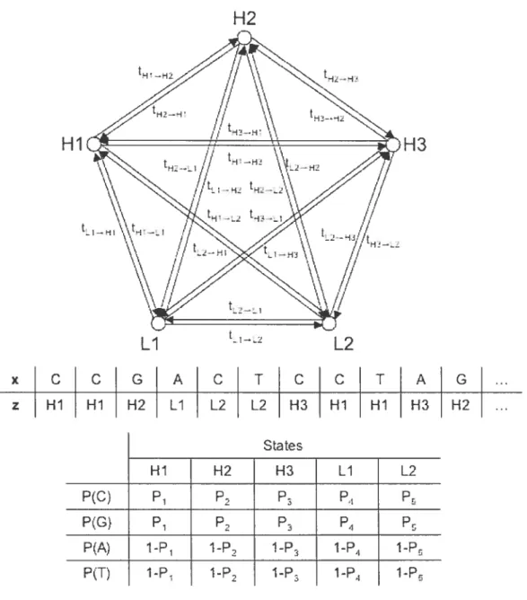
Bernaidi et aï. described tire birman genome as a mosaic of segments representing isodhores (Bernarcli 2000: Bernardi 2001). Frirthermore. their researcli reveaied that tirere are five different classes of isochores in the humari genome that are defined by

their GC-ievels: Hi. H2. H3. Li. and L2. Figure 3.1 iliustrates how tire isochore

structure of the genome cari modeiied by a hidden Markov model. The different

isochore classes are tire states.

Now. using M(z) P {X = x. Z = z} from Eqiration 3.8, the joint probabiiitv

can be written as

P{Xr=x,Zz=z} = P{X=xZ=z}P{Z=z}

= WziP(ii)t1—2ïi.(tr2)tZ.2_Z3 . . . (c). (3.12)

3.3 Complexity Penalties

Tins section reviews some alternatives to imposing prior probabilities in order to han— die tire overfitting wlren maximizing tire hkehhood. Tire basic idea is to maximize the

surir of tire iog-likehirood and a so-caiïed compiexity penalty. We discuss tirree penal ization niethods: Akaikes information criterion. tire Bayesian information criterion,

and tire priincipie of minimunr description iength.

3.3.1 Akaike’s Information Criterion

The irraximum hkelilrood principie is encountered in two clifferent brairches of statis ticai tireories: estiiïration tireorv through tire maxinrunr hkehhood methoci. aird test

(39)

21

HI

z Hi Hi H2 Li

H2

H3

L2 L2 H3 Hi Hi H3 H2 Sta tes

Figure 3.1. An example of HMM modelling isochores in that the actual isochores found in the human genome those depicted here.

human genome. Note are rnuch longer than

x C C G A C T C C

Hi H2 H3 Li L2

P(C) P2 P P4

P(G) P1 P2 P4 Pr

P(A) 1-P1 i-P i-P2 1-P4 1-Pu 1-Pi j-P2 i-3 1-P

(40)

obtained from niaximiim likeiihood estimates are most sensitive to smail variations

of the pai ameters around file truc statistical moclel. As an estimate of a measure of

fit of a statistical model. lie proposed an informatioll criterion tAlC). which cari Le described as an extension of file maxinmm likelihood principle for problems in which

the final estimafe of a fiinte paiameter moclel can Le calculated when presented al ternative maximum likelihood estimates from varions restrictions of the model. For tus paper, we coilsider “Akaikes information criterion’ as an equivaleiit terni fo ‘a11

information crit erion

Akaike used the Kullback-Leibler divergeilce function to finci the minimum differ ence between two probability distributions. namely. flic truc and approximate seg— mentation modeÏs. Suppose we use a DNA sequence x =

r1.r9

...i:7, as a sequence of

observed vaines of a sequence of randomvariables X = X1X0 ...X and a sequence of

hiddell variables z z1z2 ... z that clefines the segments. where z

e

{O — 1}

and z is clerived from a random variable Z Zy Z2 ... Z. As well. we define

f

(x)

P{X xZ z*} and g(x) P{X xZ z} where z is the truc seg

mentation anci z the approximate. Then. flic Kullback-Leibler divergence function

can Le written as

KL = f(.r)logL

=

f(:r)

log(f(:r))

- j(a) log(g(r)) (3.13)

Note that the first terni of Equation 3.13 is flxed since there cari Le only one truc

segmentation probability model. Also. notice tiiat if the approximate segmentation

probability model is the sanie as the truc moclel. that is. if

q(x)

is the saine as

,f(x).

then the Kullback-Leibler divergence will Le zero. Tins clemonstrates that the model with minimal Knllback-Leibler divergence will Le considered as the Lest estimated sequence z.

(41)

26

To obtain the optinmm estimated sequence z. Akaike suggested that we can de

termine the linear approximation of Equation 3.13 by taking the second—terni as an approximation to Akaik&s Information Criterion. that is.

AIC logL(z) — A (3.14)

where the model wliose AIC value is largest will be cliosen to represent the sequence

z. We define 771 as flic rmmber of segments in the segmentation defined by z and A as

the model dimension. Note that Equation 3.14 was multipled by —2 in the original

paper presented by Aka.ike and considered as Akaike’s information criterion due to historical reasons’ (Burnliam and Anderson 2004). In our case. z can be clescribed by a list of pairs of palameters (i.e., segnient lengtli. segment class) for 177 segments,

so we write the model dimension as A 2177. Hence. AIC can be rewritten from

Equation 3.14 as

AIC = logL(z) —2777. (3.15)

3.3.2 Bayesian Information Criterion

Akaike present cd the AIC as an extension of the maxinnim likelihood principle.

Schwarz took a similar approacli and consicÏered the problem in terms of Bayesiai

statistics (Scliwarz 1978). In contrast to Akaikes information criterion. the Bayesian information criterion (BIC) suggests that the model dimension slioulcl be multipÏied

by log n. Hence. the BIC can be written as

BIC = logL(z) — Alogn. (3.16)

The segmentation z whicli maximizes the BIC of Equation 3.16 is cliosen as flic opti

mal one. As before. we consider the length and the segment class as our parameters

(42)

model dinieusion to rewrite the BIC as

BIC logL(z) — ni logu. (3.17)

3.3.3 Minimum Description Length

Another possible approacli to measming complexity bias is through the miiirnum de

scription lellgth (MDL) method. Rissaneri (1983) preseiited tins concept hy attempt ing to find the estimate that minimizes the total number of binary digits required to rewrite the observed data, where eadh observation consists of a precision value. For a fixed segmeiltation z, an optimal encoding uses —10g2 Pz (r) bits ou a.verage

to encode flic character x in every position . Furthermore. log2 ‘n bits can be used

to encode flic length of one segment. and log2 k bits to specify ifs class. Hence. flic

total code length eau lie written as

Q = (_ log2p(.7)) + m(log9 n + log9 k) (3.1$)

wliere ni is the nuniber of segments iiï file segmentation defined by z. Equation 3.1$ can rewritten as

Q = L11ogp,(a) — m(logn +logk)

(3.19) log2

Referring to Equation 3.19, the minimum description lengtli concept woulcl maximize file immerat.or. Notice that by doillg tus, the first terni corresponds f0 tlie log— likeliliood frmction ancl the second tenu eau lie iuterpreted as a penalty on model complexity:

(43)

Chapter 4 Algorithmic Problems In

$tatistical Models

4.1 Forward-Backward Algorithrn

The probabiÏity of the observed seciuece x can be caldillated by fiuicliiig the sum of the joint probability over ail possible hidden state sequences z. However, it is

lot compitationa11y feasible silice ifs time complexity is O(n h) for a hidden i\iarkov model of k sfates ami seciueuce leugth ‘n. b solve this. ail alternate ami more efficient method is throiigh the forward-backward procedure.

Let the forward variable o

_(j).

i. the probability of the partial observation

seqiience and state

j

{O. k — 1} up to index i. be

= P{:riio . r, z ₌

j}

Then. c(j) can be solved into three steps. that is

1. Initialization:

(44)

=

i

et

D z1 =j’ tkl z = k1Q +j (ï)

Figure 4.1. Illustration of operations required for computing forward variable

2. Inductioii: =

[‘

ai(J)ti_ii] Pj’(i+i), <n, — 1 O

_<j’

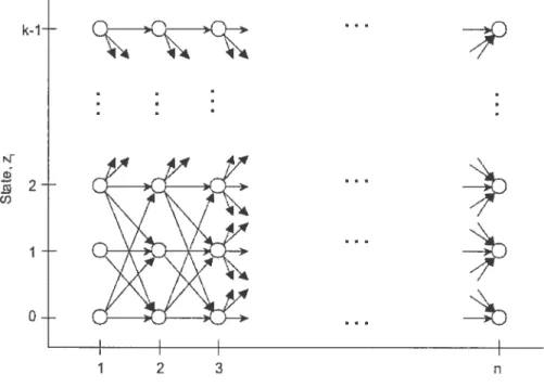
< k —1. 3. Termiriatioi: P{X=x}= i(j).

The induction step caribe illustrateci as shown in Figure 4.1, where it clemonstrates how state

_j’

cari Le reaclied at hiclex i+1 from ail possible states z

e

{O. k — 1}. where

tue transition probability observation :r÷1 in state

_j’.

anci partial observation

sequence aj(j) from ail k st.ates are taken into consideration. After flic termination step. if can be seen that the desireci calculation of P {X = x} is obtained as the sum

(45)

30 k-1 -

G.

>G—Q--4A 4% _A .2 ₂ ,/ -4 - -(f) 4 \ 4\\ \\ / I -\‘/ \‘ 4% -\

X

‘/ X Ç\ ‘X\ // \\// \_ 4 -4y_4._

o-

- )j )J 1 2 3 n Observation.

Figure 4.2. Illustration of computingcrj(j) in terms of observations x and states

of the terminal forward variables

figure 4.2 illustrates the calculations involved in the forward procedure. wliere

each state at index i+ 1 considers ail possible states z.

Similarly, let the backwarcl variable

d(j),

i.e.. the probability of the partial ob

servatioll _{seciuence from} I _{+ 1 to tue end. given} state

_J

at index I. be

/31(j)

_=j}.

(46)

1. Initialization: i3T?1. O<j<k—1. 2. Induction: /3(j) i n — Ln —2 1. j’=0 O<j<k—1. 3. Termination: P{X=x} ff13i(j). j=0

Like the induction step in the forward proced11re. Figure 4.3 demonstrates how state

j

takes ail possible states {O. k — l} into consideration. factoring iii the transi

tion probabilitv observation in state

j’.

auJ remaining partial observation

sequence ,‘3i(j’). After the termination step, P {X x} is obtained as thesum of

the terminal backward variables ,31(j).

4.2 Viterbi Algorithrn

For hidclen Markov models. the optimal state sectuence associated with

tue

given

observation sequence can foiind by implementing the Viterbi algorithm through civ—

namic programming. where eue would find a single best state sequence while takiug

several possible optimalitv criteria jute consideration.

Let z , represent the best state secjuence that is to be determined

(47)

32 _-J.D z = O -Z11 1 j z1 = k-1 +1

Figure 4.3. Illustration of operations required for computing backward variable

score, Le.

1(i)

=

Furtiiermore, let

_(j)

be the best score along a single path at index i up to state

j {O, k — 1}. i.e.,

à(j) max P{ziz2 j. :ryx. . .x}

=

m(Jf)tji_j] pj(.Tj). (4.1)

Using Eciuation 4.1. we cari iuductively find j+i(j’) as

=

(48)

where

j’

{O. k — 1}. Theil. the best sequence of hiciden variables z wheir give the

observeci sequence x cari be represented as

= argmaxP{zx}

arg maX [€fn(j)] . (1.3)

Ok—1

Let

_/‘(j’)

be an array that keeps track of the argimelÎt usecl to maximize Equation 4.2 iir order to calculate the state sequence. Then, tire Viterbi procedure can be presented as: 1. huitialization: = jpj(’i). O

j

k — 1 = O. 2. Recursion: = [à1_1(j)t]Pji(.Tj). 2 I n O

_<.1’

< k — 1 = arg max

[6_1(j)t]

2 < I n O<j<k—1 O

_<j’

<

k

—1. 3. Ternuiiiatioii:

P

= max

_[&(i)]

O<j <k—1 = arg max [S(j)].

n

(49)

34

4. Backtracking:

= ‘+i(z1), j = n — 1, n — 2 1.

4.3 Penafty-Based Best Segmentation

In this sectioii we consider the case of partitioning tlie DNA seqnence nsing tlie

penalty-based best segmentation model. Section 4.3.1 provides a description of 1ÎOW

the penalty-based best segmentation model ca be implemented using dynamic pro

gralilming. Section 4.3.2 presents tlie implemented algoritlims, witholit and witli

traceback, as well as liow flic DNA sequece can lie iteratively segmented b using

maximum—likeliliood estimation.

Let x = .. . x7, lie a seqnence of cliaracters over the alphabet Z {u1

(e.g.. a DNA seqence witli Z {A. C. G. T}). Let w1 : Z i,’ R represent a scoring

fiinction for the letters in class

j

{O k — 1}. A segmentation of x is defined by tlie segmentation inclicators z = z1 ... z7, wliere z {O k — 1}. Tlie score of sucli a segmentation is w(z) (a’). Given w1 auJ x. our main objective is to finci

z tlia.t maximizes w(z) or ifs penalized form

w(z) —

wliere o’ is a segmentation complexitv penalty. This general scori1g framework in

cincles likeliliood maximization as a specfa.Ï case: set

= _iogt _(4.4)

froni Eqiiatioii 3.3. The varions complexity penalties of Eqiiation 3.3 are reflected in

(50)

segments. A

segment

S = [a, b] _t-.

j

is

a

maximal contiguous subsequence

of

indices

{a.a+1,....b}suchthst:0=z0÷l=...=zb=j. Asegmentationset4’isdeflned as

the

partition of

the indices [1,

n]

into a set

of

segments. that is,

=

{#

.

where cadi _#j

is a segment

(and consecutive

segments

belong ta

different

classes).

4.3.1 Description

11e penalized segmentation

score takes

the segmentation penalty a

into

consideration

foreachsegmenttransitionfoundin4 andcanbewrittenasV

=

V()—a.(II—

1),

where

> O.

Lemmn

1

Let

V(Lj) be

deflned as the best segmentation score

of [1.. .i] that ends

withclassj.

Ifi>i,

then

V(i.

_j)

=w1(x,) +

max {V(i

— 1. c) —a. (4..5)

when

V(i.j) =wj(r1) and

fi

ifc#j

I.

O

othenmse

Proof Consider

the segmentation set of [i, i]

by extending

the last

intenal

of a segmentation set

associated

with V(i—i.j),

ami by adding

[Li] belonging to

class

j

to a segmentation set

associated

with V(i — i, c) where c

Ø

j.

Then.

V(i.j) w1(x1) +

max

{V(i —L c) — a,V(i— i.j)}

where

(uj(xj+V(i—i.c)—a)

anA

(wjfrj+V(4—i.j))

are

the

respective

pennhi7ed

scores. However, there is

no

inequality since

i

eau

be

removed

fitm the segmentation

(51)

36

Lemma 2 V(i.

j)

takes t’wo different cases into cons/deration: e =

j

and e

j

V(i.j) w() +max V(i — 1,j), max {VQi — 1, e)

—

cE [O.k—1]

Proof Let /3 represeut the secoiid terni of tlïe eqiiation, that is

/3 max

{vti

— 1.

j).

max{V(i — 1.c)

—

Since it is trivial that V(i — 1.

j)

> V(i — 1,

j)

— a / cail be rewrittell snch that

/3 max — Lj). max {V(i — 1, e)

—

ceO.k—1J\j

Herice. this leminas equa-tion is the same as Equation 4.5. that is.

V(i,j) = j(’) +max{V(i — 1.j). max {V(i — Le)

—

i}

= w(i) ₊ max {jT(/ — 1.e) —

cE [O.k—1]

I

Lemma 1 implies a dynamic prograninhing algoritiimi that execntes iii O(nk2) time. The implementation of Lemma 2. however. implies that the maxinifim value

of V(i — 1, e) eau be pïe-calc11lated auJ would reduce the tnne complexity to O(nk)

tillie.

4.3.2 Algorithrns

Without Traceback Implementation

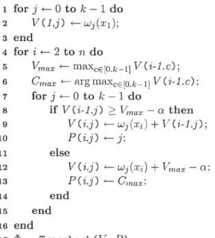
Equation 4.5 demonstrates the accrinmlatecl score calcula.tion at lÎncleoticle c Lv using the Lest Possible prefix score at the previous nucleotide :r1 via dynamic pro

(52)

scores at the first nucleoticle tr1 are iiitialized as written in the the loop body 1—3. The loop body 4-13 processes the scores of the remaining nucleotides r for cadi class. where Lille 5 helps reduce tic number of it.erations of cleterminiug the maximum value

of the scores from tic previous nucleotide. Lines $ auJ 10 are implementations of

Lemma 2 for each class.

Lemma 3 The atgoritkrn presented in Fgure

_.4

finds an optimal segmentation into k classes for o, DNA sequence of iength n in 0(nk) time.

Proof Tic iruitialization of tic scores for

j

[0.k — 1] at i1 is performeci iii tic first

loop body 1-3 in 0(k) time. Tic second ioop body 4-13 is executed n — 1 times,

where the maxinmm ofV(i — 1.c) for c

e

[0. k — 1] in Liue 5 auJ the huiler loop body

6-12 are determined in 0(k) time for cadi iteration. Tierefore, tie time complexity

eau be simplifieci to yield 0(nk).

_I

Input : Sequence X. segmentation penalty n

Output: Best perialized segmentation 1 for j — O to k — 1 do

2 V(1,j) .—wj(;i): 3 end

4 for i 2 to n do

5 dnax flillXce[ok_1] V(i-1.c) 6 forj —0 to k—1 do y if V(i-1.j) > — n then 8 V(i.j) wj(.r) + V(i-1.j): 9 else 10 V(i.j) w() + — n: ii end 12 end 13 end

(53)

3$

With Traceback Implementatioii

Let P(i.

j)

clenote an element of the tracebaek arra.v containing tire class number of the previous nucleotide r1 referreci to when calculathrg the accuumlated penalized

segmentation score l’(i.

_j)

via Equation 1.5. for example. if V(i.

j)

w(;r1) +

V(i — 1. e) — and e

j.

ther P(i.

j)

e (otherwise. P(h

j)

= j). Tire aigorithm

presented in figure 4.5 is an adapted version of algorithm clenoted in Figure 4.4 which incorporates tire traceback array feature. where P(i,

j)

is assigneci in Lhies 10 auJ

13 for each 1 < i < _{n anci ciass} _{e. Note that tire traceback array elements at the}

beginning of the sequence for each class e, that is, P(1,e) are not assigned. Line 17

assembles tire segmentation set c1 through tire traeback algorithm.

Input _{: Seciueiice X, segmentation peHalty n} O utput: Best penalized segment ation F 1 for j O to k — 1 do

2 V(1.j) 3 end

4 for j — 2 to n do

5 rncix 1Y1axro1jV(i-1.c):

6 °mci:l• arg 1riax.C[o.k_y] V(i-1.c): 7 forj—Otok—ldo 8 if V(i-1.’j) > l/ — n then 9 V(i.j) W (T) + V(i-1.j): 10 P(i.j)

+—j;

ii else 12 V(i.j) — w(x) + — n: 13 P(i.j) — 14 end 15 end 16 end 17 çFi—Traceback(V. P):

Figure 4.5. Penafty-based best segmentation with traceback array ai gorithrn.

(54)

The traceback algorithm is impÏementecl as shown in Figure 4.6, where it computes the segments obtained from

tue

pellalty-basecl best segmentation aigorithm. We use z z1 . . . z, to store the class numbers of the secluence. As well, let 6 be tue cunent

segment class number. 6’ the segment class rnuÎlber reaci from the traceback array.

start the start of a segment, end the end of a segment, and p the iterator for the Ïist

of segments. This aÏgorithm is initialized by deterniining which class contains the niaximmïi accumulated penalizeci score for

tue

sequence as illustrated in Line 4. In the loop bodv 6-10, 6’ is read from the traceback array (Line 7) and is inserted into

z1 _{(Line 9). The segmentation set F ïs assembled in the loop body 11-18, where the}

segment p = {[start.end] z_i} is inserted into ) if z1 15 not equal to z (Line

12). As well. end anci are upclated as denoted in Lines 13 auJ 15. respectiveÏy.

The last segment inserted to the list is represented in Line 20.

Maxirnum-Likelihood Estirnatioll of Segmellts

Maximum-likelihooci estimation can be used to aj proximatelv cleterniine the segments

of a given sequence when provided probability values. This can be implemented

in conjunction with the penaltv-basecl best segmentation algorithm as presented in

Figure 4.7.

The algorithm will be repeated executecl in the loop body 1-5 until the log likelihood ratio converges. For each iteration. a uew score is calculated based on

the log—likelihood ratio auJ a new segmentation is coinputecl via the penalty-based

best segmentation algorithm as presented in Figure 4.5. Furthermore. new probaÏility

values are calculated using Laplace pseudo-counters as impÏemented in the algorithm

(55)

40

Input : Segmentation score arrav V, traceback array P. penalty c Output: Assembleci segmentation cF

1 start 1; 2 _nd 1; 3 p —1; 4 Ô argmaxE[O.c_l] V(n,c); 5 z — 6; 6 for j — n downto 2 do 7 6’ P(i.6); 8 64—Ô’; 9 Z_j Ô; 10 end ii for j 2 to n do 12 if then 13 14

p {[istaro end] I”

15 _start 1— j: 16 p—p+l; 17 end 18 end 19 ij — n; 20 _p 4- {[start,end] ‘

Figure 4.6. Traceback algorithm.

Input : Sequence X. segmentation penalty n

Output: Maximum-likelihood segmentation via penaÏty-based best segmentation

algorit 11m (J) 1 repeat 2 wjr)1og-; 3 cF BestSegmentation(X. o): 4 p ProbabilityCalculation(cF); 5 until convergence

Figure 4.7. Maximum-iikelihood estimation of segments via penalty based best segmentation algorithm.

(56)

4.4 Penalty-Based Best Segmentation with Mini

mum Segment Lengths

Intins sectionwe discuss the case of partitioning the DNA segrience using the penalty—

based Lest segmentation with minillmm segment lengths model. Section 4.4.1

prO-vides a description of how the pellalty—based Lest segmentation with mimimum seg ment iengths model cari be impiemented using dynamic prograilming. Section 4.4.2 presents tire implemented algorithms without and with traceback. as weil as air algo—

rithm in which tire DNA sequence cari Le iteratively segmenteci by using maximum—

iikeiihood estimation.

4.4.1

Description

\\‘iule calculating via tire penalty-based Lest segmentation eciuatio;r as presented in Equation 4.5 vielcis a pattern of segments in tire seqnence, it is possible that overfitting

data (i.e. [i i]

j

: > O segnients) cari occur and consequentiy render the

data hiologicaliy meaningless. Hence. Equation 4.5 cari Le modlifled sucli that it takes minimum segment Ïeiigths into consideration.

Let rn Le ciefined as tire minimmrr segment iength for ciass

j.

Thtis. for ni g

[1.mi], and j g [m, n], iet _m represent tire segmentation sets of [1, j] that maximize V(cF) whuie satisfying tire requirements for ail segnrent ierigths except for the iast one of class

j

whose length is at ieast in.

Lemma 4 Let iiort(i.j) = V((I1) _{and ong(i.}

j)

V(I711

).

TÏierefore, flic fol

towing rec’ursions represent

tue

caÏc?itation of th e weights of these segmentation sets.

that îs

1iwrt(.j) ₊

max

{

/rnri( — 1.. max {409(i — 1. e) — (4.6)

(57)

42

9(i,j) = — m + 1.

j)

+ w(xt) (4.7)

l=i—7fl)+2

where “ïiort(1.j) = w1cri) and e [O. k — 1]

\ j.

Proof For Equation 4.6, let Ç5s1?ort lie some segment of cÏass

j

al rnic1eoticlex, i.e.

short [i. i] j,’

j.

If tire last segment cf F includes micleotide — (i.e. nucleoticle

a and — are of the same nueleotide). then is obtained liy extencling tire last

Segment cf Otherwise. F1 ₌ CFlfl? U _{s1iort}.

for Equation 4.7, let _loT?g lie sorne segment of class

j

from nucleotides

t.o x, i.e. _tong [i —fuj + 2. j]

j.

(Fm is olitained liy ext.ending tire last segment

cf _{rn3H-1.1 Witi} segment _5long

_I

Lemma 5 Vsor takes t’wo different cases jnto cons/deration: e =

j

and e

j

iort(j,j)

1Cr)

₊ max _{ïzori( —

cij{ong(i

— 1. c) — o}}

Proof Let /3 represent the second terni of the equation. that is

= max _{hOit( — 1.j).

c.Ij {orig(’

— 1. e) —

Let mlor?g lie tire requireci minimum segment iength associateci with ‘ong(—1.

j)

—

Likewise. let ms/iort = 1 lie the required minimum segment iength associated with

Vshort( — 1.

j).

$ince lÏong ??ishort. then

— 1.

j)

> ouig( — 1.

j)

—

1-lence, /3 eau lie rewritten such that

/3 = niax

{

1jo( — L

j),

{i)ong( — 1. e) —

(58)

Therefore, this len;n;as equation is the same as Equation 4.6. that is,

hori;(Z,J) w() + max iwrt( — U). max {iong(i — 1. e) — = max

{

UshorttZ — 1, cl] {4ong(i — 1. e) — o’

}

I

Lemma 4 implies a dynamic programming of that computes an optimal segmen tation set that is subject to the given minimum segnïent lengths in 0(nk2) time. However. like Lemma 2. applying Lemma 5 would allow the pre—calculation of the

maxinium vaine of (i — 1. c). thereby reducing the time complexity to 0(iik).

4.4.2 Algorithms

Without Traceback Implernentation

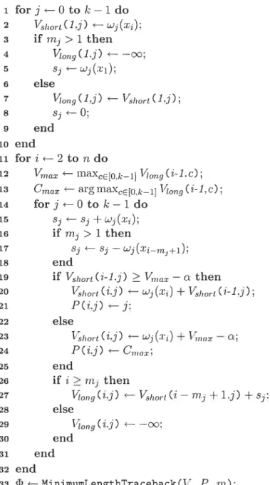
Referring to Equations 4.6 and 4.7. the occurrence of overfitting data cal; be elinu

nated by specifving

tue

minimum segment lengths of segments. Let ni be ai; array

containing mininmn; segnïent lengths for cadi class

j.

Tic algoritim presented iii Figure 4.8 illustrates tins computation where both Vsh and i’ scores at the first nuc1eoticler are initiallzed for cadi class in tic loop bociv 1-10. Loop body

11-29 processes fie scores of the remaining nucleoticles .r, wiere fie largest value of

iong( — 1, e) is cletermineci in Line 12 in orcler to reduce tic nllmber of required

iterafions. Tic muer 1001) bodv 13-28 is ai; implementation of Equations 4.6 and 4.7.

Lemma 6 Tue aÏgoritkn; presented in figure .8 finds an optirnaÏ segmentation into

k classes for a DNA sequence of leu gth n in OQk) time.

Proof lie initialization of tic scores for

j

[0. k — 1] at r1 is perfornied in tic

(59)

44

times, where the maximum calciilations in Line 12 and the illiler loop body 13-2$ are

determined in 0(k) time for each iteration. Therefore, the time complexity cari Le

simplified to yield 0(71k).

Input : Sequence X. segmentation penalty , millirnum segment lengths ‘rn

Output: 1\Iinimrim length segmentation 1

1 for j O to k — 1 do 2 VSÏ?OTt(1.i) ‘ 3 if mi > 1 then 4 Vog(1.j) — —oc; 5 s ‘ wi(ri); 6 else ong(Lj) ‘ Vswrt(1,j): 8 _si—O: 9 end 10 end ii for i *— 2 to ‘n do 12 “ rnaxCE[t).I,_l) ‘Lng(il.c); 13 forj—Otok—1do 14 _si 5 15 j > 1 then 16 _s _s — end 18 if (i-i,j) —c then

19 _Vshort(i.j) wi(:ri) + (i-1.j);

20 else

21 _hort(i.j) ‘ wj(x) + 1’nax — n:

22 end 23 if i _ii then 24 _1ong(z.j) ‘ hort(i — rn+ 1,j) +sj; 25 else 26 Vonq(i.j) ÷— —oc: 27 end 28 end 29 end

Methods for multi-class segmentation of molecular sequences