1
Using remote sensing to characterize
riparian vegetation: a review of
available tools and perspectives for
managers
Leo Huylenbroeck1*+, Marianne Laslier²*, Simon Dufour3, Blandine Georges1, Philippe Lejeune1, Adrien Michez1
*Contributed equally
+
Corresponding author (leo.huylenbroeck@uliege.be)
1
ULiège, Gembloux Agro‐Bio Tech, TERRA Teaching and Research Centre (Forest is Life). 2, Passage des Déportés, 5030 Gembloux, Belgium
² INRAE centre de Lyon Grenoble Auvergne Rhône-Alpes. 5 Rue de la Doua, 69100 Villeurbanne, France
3
2 Research Highlights
Review shows diverse approaches and objectives for mapping riparian vegetation Scale of observation, remote sensing data and mapped features are strongly related Finer spatial and temporal resolution will renew large scale and diachronic analyses We discuss the challenges of conveying remote sensing tools to managers
3
Abstract
Riparian vegetation is a central component of the hydrosystem. As such, it is often subject to 1
management practices that aim to influence its ecological, hydraulic or hydrological functions. 2
Remote sensing has the potential to improve knowledge and management of riparian vegetation by 3
providing cost-effective and spatially continuous data over wide extents. The objectives of this 4
review were twofold: to provide an overview of the use of remote sensing in riparian vegetation 5
studies and to discuss the transferability of remote sensing tools from scientists to managers. We 6
systematically reviewed the scientific literature (428 articles) to identify the objectives and remote 7
sensing data used to characterize riparian vegetation. Overall, results highlight a strong relationship 8
between the tools used, the features of riparian vegetation extracted and the mapping extent. Very 9
high-resolution data are rarely used for rivers longer than than 100 km, especially when mapping 10
species composition. Multi-temporality is central in remote sensing riparian studies, but authors use 11
only aerial photographs and relatively coarse resolution satellite images for diachronic analyses. 12
Some remote sensing approaches have reached an operational level and are now used for 13
management purposes. Overall, new opportunities will arise with the increased availability of very 14
high-resolution data in understudied or data-scarce regions, for large extents and as time series. To 15
transfer remote sensing approaches to riparian managers, we suggest mutualizing achievements by 16
producting open-access and robust tools. These tools will then have to be adapted to each specific 17
project, in collaboration with managers. 18
Keywords
19
Riparian forest, alluvial forest, floodplain vegetation, LiDAR, UAV, satellite 20
4
1. Introduction
22
At the interface between terrestrial and aquatic biota, riparian vegetation is a central element in the 23
hydrosystem, where it plays many ecological roles and interacts with all hydrosystem components 24
(Naiman et al., 2005). In a broad sense, riparian vegetation corresponds to all vegetation types that 25
grow within the area influenced by a river network (Naiman and Décamps, 1997). 26
Despite covering a relatively small area, riparian vegetation provides many ecosystem services 27
related to river flow (Dixon et al., 2016), sedimentary processes (Zaimes et al., 2004), biodiversity 28
(Naiman and Décamps, 1997), water quality (Honey-Rosés et al., 2013, Brogna et al., 2018), cultural 29
value (Décamps, 2001, Klein et al., 2015, Vollmer et al., 2015). However, riparian ecosystems 30
experience multiple pressures (e.g. land use, water diversion, modified flood regime) (Stella and 31
Bendix, 2019) and have been severely altered in many regions of the world, for example in Western 32
Europe (Hughes et al., 2012), southwestern North America (Poff et al., 2011), in the Murray‐Darling 33
Basin in Australia (Mac Nally et al., 2011) or in South Africa (Holmes et al, 2005). Consequently, 34
riparian vegetation is often the focus of management practices, including restoration or 35
rehabilitation measures (Dufour and Piégay, 2009; González et al., 2015; Capon and Pettit, 2018), 36
buffer implementation (Lee et al., 2004) or repeated maintenance operations such as wood removal 37
(Piégay and Landon, 1997; Wohl et al., 2016). 38
In this context, management practices must be based on accurate and up-to-date information about 39
the state of riparian vegetation (National Research Council, 2002). Regional or national programs 40
have thus been established in many countries to monitor the health of riparian ecosystems. 41
Examples include southern Belgium (Debruxelles et al, 2009), Spain and more generally the European 42
Union in the frame of the Water Framework Directive (Munné et al., 2003, Willaarts et al., 2014), 43
Australia with the South East Queensland Healthy Waterways Partnership (Bunn et al., 2010) or the 44
monitoring of riparian condition in several National Parks in North America (Starkey, 2016). Dense 45
sampling schemes can help target and implement management practices (Landon et al., 1998; 46
5 Beechie et al., 2008) or assess their effectiveness (González et al., 2015). However, due to the spatial 47
arrangement, dynamism and inaccessibility of riparian ecosystems, data acquisition in the field can 48
be labor-intensive, especially for large areas (i.e. more than 100 km of a river) (Johansen et al., 2007). 49
It is thus difficult to sample densly in the field, and the density or the extent of observations must be 50
reduced. This can be problematic, because river scientists argue that small scale or discontinuous 51
observations are inadequate to understand spatially continuous processes that occur at large spatial 52
scales (Fausch et al., 2002; Marcus and Fonstad, 2008; see also Tabacchi et al., 1998 or Palmquist et 53
al., 2018 for examples related to riparian vegetation). 54
Remote sensing provides the ability to acquire continuous data over large extents. In the past few 55
decades, the continued development of sensors, vectors and computational power has fueled the 56
development of applications in environmental science (Anderson and Gaston, 2013; Wulder et al., 57
2012). The positive contribution of remote sensing to the management of natural resources is 58
adressed by many articles related to river or riparian management (Carbonneau and Piégay, 2012, 59
Dufour et al., 2012). This is not only a theoretical issue as is it regularly raised by riparian managers in 60
the grey literature (Vivier et al., 2018, Fédération des Conservatoires d’espaces naturels, 2018). 61
However, it is difficult for managers to know whether and which remote sensing methods are 62
relevant to a particular situation (Dufour et al., 2012). 63
The use of remote sensing to study riparian vegetation raises specific challenges. These challenges 64
are linked to the vegetation’s relative structural complexity and spatial organization (Naiman and 65
Décamps, 1997), or to the difficulty to extract specific features or processes related to riparian 66
vegetation functions (e.g. surface roughness by Straatsma and Baptist (2008), shading of streams by 67
Loicq et al., 2018). In a recent literature review, remote sensing emerged as a particularly dynamic 68
subject in riparian studies (Dufour et al., 2019). Remote sensing of riparian vegetation was 69
mentioned in several reviews addressing the remote sensing of rivers (Muller et al., 1993; Goetz, 70
2006, Tomsett and Leyland, 2019, Piégay et al., 2020). Specific aspects were also reviewed such as 71
6 the mapping of roughness coefficients with remote sensing (Forzieri et al., 2012) or the use of 72
satellite images to map riparian vegetation in New Zealand (Ashraf et al., 2010). Dufour et al. (2012) 73
and Dufour et al. (2013) summarized and discussed several examples of remote sensing applications 74
to map riparian vegetation. However, none of the aforementioned articles comprehensively 75
reviewed the use of remote sensing to map riparian vegetation across regions, scales and 76
researcher’s interests. Indeed, the latter are fragmented among several fields of knowledge (e.g. 77
ecology, geomorphology or hydraulics) (Dufour et al., 2019). 78
The aims of this article are 1) to provide a comprehensive overview of the relevance of remote 79
sensing to support the study of riparian vegetation and 2) to discuss how remote sensing approaches 80
can be valued as operational tools for managing riparian vegetation. To these ends, we first 81
systematically review the different types of data used to study major features, functions and 82
processes related to riparian vegetation across scales (section 3). The second part of the article 83
(section 4) is based on expert judgment. We provide concrete examples where remote sensing is 84
used in management contexts, in order to identify the challenges of conveying remote sensing tools 85
from scientists to managers. 86
2. Materials and methods
87
Our approach was structured as following: we first selected relevant articles in the Scopus database. 88
Second, relevant information was extracted for each article, and summarized into graphs. Our results 89
were discussed in terms of trends and perspectives for research, and in terms of operationality and 90
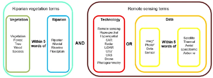
transferability to riparian managers. The Figure 1 synthesizes our approach. Major steps are further 91
detailed in the following sections. 92
7 93
Figure 1. General workflow for the reviewing process
94
2.1. Database collection
95Relevant articles were selected from the Scopus database (www.scopus.com) for the period 1980 - 96
April 2018, when the database was queried. We searched the title, abstract and the keywords for 97
words related both to riparian vegetation and to remote sensing technologies. More precisely, we 98
used the request described in the Figure 2. 99
100
Figure 2. Keywords used for database collection
8 Our choice of keywords excluded articles that mentioned riparian zones, but not specifically riparian 102
vegetation. While some of these articles could have been relevant for this review, including keywords 103
related to riparian zones would have resulted in unmanageable noise. 104
This request yielded 791 articles. We first filtered out irrelevant articles based on their title (672 105
articles kept). Then, we sorted through the remaining articles based on their abstracts (428 articles 106
kept). During these two filtering steps, we removed mainly articles in which riparian vegetation was 107
not an essential part of the study. For example, we removed geomorphological articles in which 108
riparian vegetation was mentioned in the abstract but was not actually studied. Articles that used GIS 109
but no remote sensing data were also removed (e.g. those using cadastral archives). 110
We also built a second database using only keywords related to riparian vegetation, excluding those 111
related to remote sensing. This second database was solely used to estimate the proportion of 112
remote sensing studies among riparian vegetation studies, and was not analyzed using the analysis 113
grid described in the following section. 114
2.2. Analysis grid
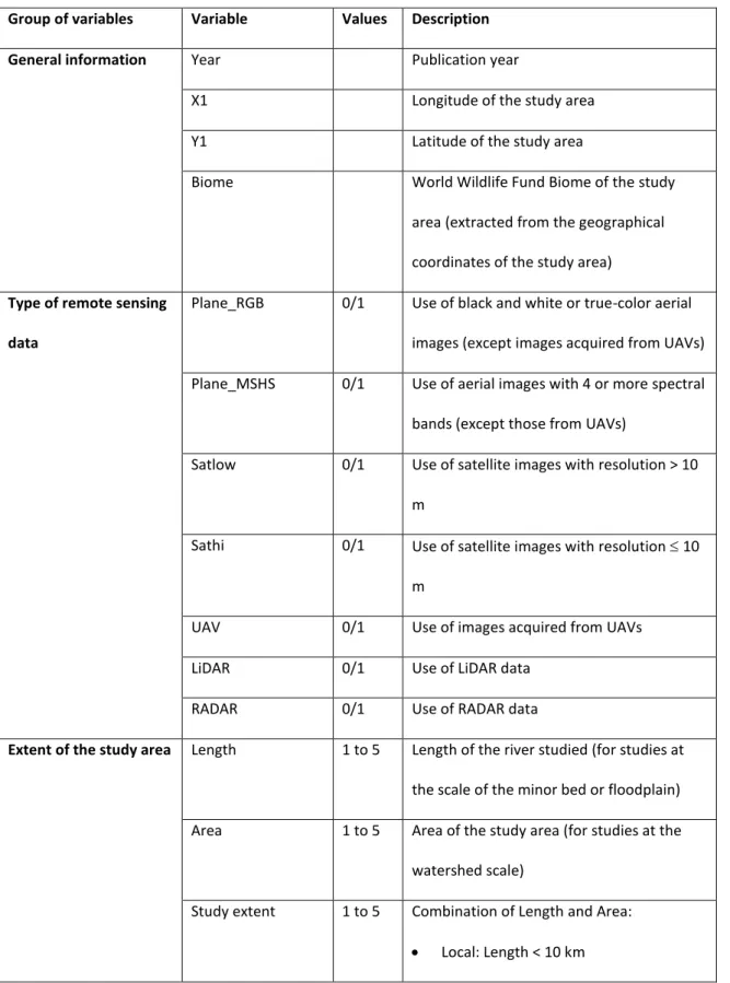
115We searched for features that characterized the articles collected to perform quantitative analysis 116
and statistics. We built our analysis grid (Table 1) around five groups of variables: “general 117
information”, “remote sensing technology”, “study extent”, “type of indicator” and “multi-118
temporality”. In this paragraph, when not obvious, we highlight in bold the codes (used in figures) 119
associated with the variables. ”General information” included variables such as the publication year 120
and location of study area. “Remote sensing technology” described the type of remote sensing data 121
used. To simplify interpretation, we recorded this information as common combinations of sensors 122
and vectors. We distinguished the following: airplane with a RGB/GS (red-green-blue or 123
panchromatic), digital or analog sensor (Plane_RGB); airplane with a multispectral or hyperspectral 124
sensor (Plane_MSHS); UAV with any sensor (UAV); any vector with a LiDAR sensor (LiDAR); any 125
vector with a RADAR sensor (RADAR) and satellite with a multispectral or hyperspectral sensor. This 126
9 last variable was coded according to image resolution: medium (> 10 m, Satlow) or high (≤ 10 m, 127
Sathi). ”Study extent” described the extent of the study area as the length of studied river or area of 128
the study area. These two variables were recorded in categories and then summarized into a single 129
category to simplify interpretation: study extent. “Type of indicator” described the type of features 130
extracted with remote sensing data to describe riparian vegetation. Delineation of riparian 131
vegetation among other land cover types (DLC) is the first feature extracted for managing riparian 132
vegetation. Species composition is a major feature of riparian plant formations. It is related to 133
habitat provision, bank stabilization and flood regulation functions; for example, willow is a pioneer 134
species that helps to stabilize banks (Hupp, 1992). We distinguished studies that differentiate groups 135
of species (Communities) and studies that differentiate species (SP). We also distinguished studies in 136
which the target species were invasive (SP_invasive), since riparian zones are particularly prone to 137
invasions (Richardson et al., 2007). We distinguished studies in which the target communities were 138
succession stages, since riparian systems are pulsed systems in which succession is regularly 139
reinitiated, leading to a mosaic of succession stages (Kalliola and Puhakka, 1988). The structure of 140
riparian vegetation is related to many ecological functions. We recorded general descriptors of 141
vegetation structure such as vegetation height, density, biomass and landscape structure. We also 142
recorded studies interested in hydraulic properties of vegetation (Roughness), since riparian 143
vegetation has tremendous effects on the hydraulic regime of rivers, especially by slowing river flow 144
(Curran and Hession, 2013). Riparian shade (or overhang) influences fish habitats and is a major 145
factor regulating stream temperature (Poole and Berman, 2001). Large woody debris (LWD) has 146
many effects on provision of aquatic habitats, river morphology and flood risk prevention (Wohl, 147
2017). Features related to physiological processes, including phenology and health statuts (e.g. tree 148
dieback), are a major concern for managers (Cunningham et al., 2018). Riparian evapotranspiration 149
has often been studied in arid or semi-arid systems because it has a major effect on providing water 150
for human use (Dahm et al., 2002). ”Multi-temporality” included only one variable (Diachronic), 151
which corresponded to a special type of study diachronic analysis that uses a temporal series of 152
10 images to describe vegetation dynamics. We recorded all variables as presence/absence data to 153
capture the use of several types of data or the mapping of several indicators in the same article. 154
Table 1. Analysis grid used for each article in the database
155
Group of variables Variable Values Description
General information Year Publication year
X1 Longitude of the study area
Y1 Latitude of the study area
Biome World Wildlife Fund Biome of the study
area (extracted from the geographical coordinates of the study area)
Type of remote sensing data
Plane_RGB 0/1 Use of black and white or true-color aerial
images (except images acquired from UAVs)
Plane_MSHS 0/1 Use of aerial images with 4 or more spectral
bands (except those from UAVs)
Satlow 0/1 Use of satellite images with resolution > 10
m
Sathi 0/1 Use of satellite images with resolution 10
m
UAV 0/1 Use of images acquired from UAVs
LiDAR 0/1 Use of LiDAR data
RADAR 0/1 Use of RADAR data
Extent of the study area Length 1 to 5 Length of the river studied (for studies at the scale of the minor bed or floodplain)
Area 1 to 5 Area of the study area (for studies at the
watershed scale)
Study extent 1 to 5 Combination of Length and Area:
11 River segment: Length 10-100 km OR
Area < 100 km²
Subregional: Length 100-1000 km OR Area 100-1000 km²
Regional: Length > 10,000 km OR Area 1000-10,000 km²
Very large scale: Area > 10,000 km²
Type of indicator
Delimitation DLC 0/1 Mapping of riparian vegetation (including
land cover studies) Species
composition
Communities 0/1 Mapping of several distinct riparian plant
communities
Succession stages 0/1 Mapping of several succession stages
SP 0/1 Mapping of riparian vegetation at the
species level
SP_invasives 0/1 Mapping of invasive species
Vegetation structure
Height 0/1 Mapping of vegetation height
Landscape 0/1 Calculation of landscape metrics (e.g.
continuity)
Density 0/1 Mapping of vegetation density
Shade 0/1 Mapping of shade cast by vegetation
Biomass 0/1 Mapping of biomass
LWD 0/1 Large woody debris (wood in rivers)
Roughness 0/1 Mapping of vegetation hydraulic properties
Physiological processes
Evapotranspiration 0/1 Estimate of vegetation evapotranspiration
Health status 0/1 Mapping of vegetation health status (e.g.
tree dieback, defoliation)
Phenology 0/1 Mapping of vegetation phenology
12
2.3. Statistical analysis
156
We computed the annual number of published studies using remote sensing of riparian vegetation. 157
We also computed for each year the proportion of studies that used remote sensing among all 158
riparian vegetation studies. To do so, we compared the number of articles in the database related to 159
remote sensing and riparian vegetation with the number of articles in the database related to 160
riparian vegetation in general. 161
The data collected with the analysis grid were summarized and plotted. We computed the number of 162
articles for each WWF biome, the use of different remote sensing technologies through time. We 163
then compared the use of different technologies according to the scale of observation, the indicator 164
extracted and the multi-temporal character of studies. 165
Finally, we performed a multiple correspondence analysis in order to highlight relationships between 166
the type of data and the type of feature extracted. We used the package FactoMineR of R software. 167
All variables were recorded as categorical variables. Variables related to study extent and multi-168
temporality were added as supplementary variables. 169
2.4. Interpretation of results
170Results were discussed in two phases. First (section 3), we use our quantitative review of the 171
literature to establish the state of the art and main perspectives in the use of remote sensing to map 172
riparian vegetation. Second (section 4), we discuss how remote sensing can be used in real 173
management contexts. We first discuss the added value of remote sensing in such contexts using 174
concrete examples from the grey literature and personal experience. Then, we use these examples to 175
discuss the challenges that must be overcome in order to promote the use of remote sensing by 176
riparian managers. Therefore, while the section 3 of this article is based on a rigorous review of the 177
scientific literature, the section 4 of this article is rather based on expert judgment. 178
13
3. Results and discussion of the systematic review
179
3.1. Location of the studies
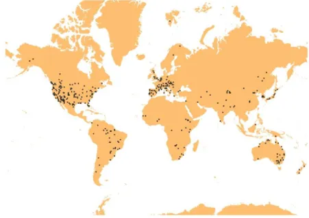
180Most studies in the 428 selected layed in the Northern Hemisphere (79%), especially in North 181
America (40% of studies) and Europe (20% of studies) (Figure 3). South America, Oceania, Asia 182
(mostly Japan) and Africa represented respectively 9%, 9%, 11% and 5% of studies. Most represented 183
biomes (Figure 4) were hardwood and mixed temperate forests (28%), temperate coniferous forests 184
(14%), and deserts and xeric bushes (13%). Mediterranean biomes (10%) and temperate open 185
biomes (8%) were also well represented. Well-represented biomes generally corresponded to those 186
in developed countries. Conversely, boreal forests and tundra were least represented (< 1% of 187
studies), though they cover a large area globally (> 10% of emerged land area). In addition, despite 188
the large extent of tropical biomes (tropical and equatorial forests or open vegetation, ca. 30% of 189
emerged land area), few studies focused on them. 190
191
Figure 3: Locations of the study areas of the studies reviewed
14 193
Figure 4. Locations of studies reviewed, by World Wildlife Fund biome
194
This result highlights the lack of knowledge and studies about tropical and boreal riparian forests, 195
perhaps due to the location of laboratories, which are often located in developed countries and 196
temperate climates. Our results are similar to those of Dufour et al. (2019) for all riparian vegetation 197
studies and those of Bendix and Stella (2013) for studies of vegetation/hydromorphology 198
relationships. 199
However, we suggest that the increasing quality of remote sensing data has great potential for 200
research in understudied areas and at the global scale. One condition is that these data must be 201
available to their potential users. Open or free remotely sensed data, such as Landsat, MODIS or, 202
more recently, Sentinel images, allow researchers to overcome the issue of the prohibitive cost of 203
data acquisition. This is particularly true for researchers in developing countries for data that are 204
produced in wealthier countries (Sá and Grieco, 2016). However, to broaden the user base, it is also 205
necessary to facilitate access to these data (Turner et al., 2015). Access can be facilitated by 206
providing higher-level (e.g. atmospherically corrected) or derived products, such as global land cover 207
maps (Gong et al., 2013), global floodplain models (Nardi et al., 2019) and maps of riparian zones 208
15 (Weissteiner et al., 2016, at the European scale). Access can also be made easier by developing an 209
open, free or user-friendly environment to find, visualize and process data (Turner et al., 2015). 210
3.2. Changes over time in the number of studies that used remote
211sensing to study riparian vegetation
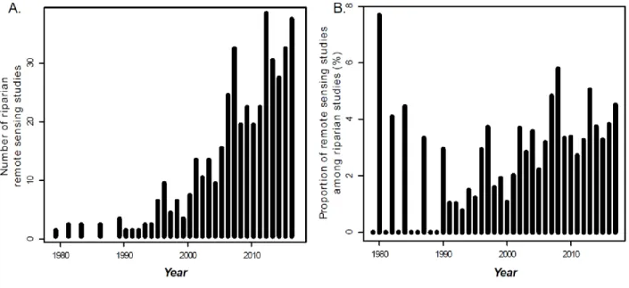
212Most of the 428 studies (89%) that used remote sensing to study riparian vegetation from 1980-2018 213
were published after 2000 (Figure 5A), when the number of studies began to increase greatly. Before 214
1990, few studies used remote sensing to study riparian vegetation. The percentage of studies using 215
remote sensing among studies studying riparian vegetation increased in the 2000s (Figure 5B). Each 216
year after 2000, 2-6% of all studies of riparian vegetation used remote sensing. Thus, even recently, 217
relatively few studies use remote sensing data to study riparian vegetation, and field-based 218
approaches dominate riparian vegetation studies despite the development of remote sensing and 219
modeling approaches. This could be due to three main reasons. First, field-based approaches have 220
traditionally been used and are straightforward. Some aspects of riparian vegetation, such as 221
biogeochemical functioning and soil properties, cannot realistically be studied with remote sensing 222
(Dufour et al., 2012). Second, the spatial structure of riparian vegetation makes it difficult to study 223
using remote sensing. Its complexity (Naiman et al., 2005) and narrow shape is difficult to observe 224
with low resolution satellite images (Johansen et al., 2010). Additionally, the linear shape of riparian 225
corridors requires acquiring images over large areas (to cover sufficient corridor length), only to focus 226
on small areas (near the river, rather than other land cover classes). For example, Weissteiner et al. 227
(2016) estimated that Europe's riparian area represented ca. 1% of its total continental area. Third, 228
we removed duplicate and irrelevant articles from our database, but did not do so when identifying 229
all articles describing studies of riparian vegetation in general, which may have led us to 230
underestimate the percentage of all riparian studies that used remote sensing. 231
16 232
Figure 5. A: Number of studies from 1980-2018 that used remote sensing to study riparian vegetation. B: Percentage of
233
studies from 1980-2018 that used remote sensing, out of all studies concerning riparian vegetation (see section 2.3).
234
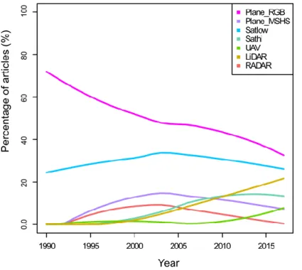
3.3. Changes in remote sensing data over time
235The remote sensing data used most were aerial RGB/GS images (44% overall) and medium-resolution 236
satellite images (> 10 m resolution, and ≤ 50 m for most studies) (Figure 6). Aerial multispectral 237
images appeared in the 1990s and peaked during the 2000s. The use of high resolution satellite data 238
(≤ 10 m such as IKONOS, SPOT 5 and WorldView) started in the late 1990s and reached a plateau 239
around 2010. The use of LiDAR data consistently increased during the 2000s, accounting for 20% of 240
studies using remote sensing for riparian vegetation in 2017. The use of UAV images sharply 241
increased in the 2010s. As the use of these technologies increased, the percentage of studies using 242
RGB/GS aerial images and low resolution satellite images decreased slightly. Overall, less than 2% of 243
studies used RADAR data. Their use peaked in the early 2000s and then decreased. 244
17 245
Figure 6. Percentage of studies that used a given technology per year. The curve was smoothed using a loess regression.
246
The popularity of RGB/GS aerial and low resolution satellite images can be explained by their low 247
cost and wide availability, including as time series. Other data have been used as they became 248
available (e.g. LiDAR and high resolution satellite images in the 2000s, UAVs in the 2010). The relative 249
decrease in the use of multispectral aerial images could be due to their replacement by high 250
resolution satellite images. Finally, the low percentage in the use of RADAR data could be due to the 251
relative difficulty of interpretation of such data, especially as water surfaces can modify RADAR 252
signals. Most studies in our database that used RADAR data focused on the interaction between 253
water and riparian vegetation, mapping flooding events or roughness coefficients (Townsend, 2002). 254
The early decrease in the use of RADAR data coincides with the increase in the use of LiDAR data, 255
which also provide structural information. 256
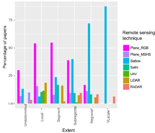
3.4. Which technology for which study scale?
257There was a strong relationship between the scale of the study (local to very large scale) and the type 258
of remote sensing data used (Figure 7). In general, aerial images were used more at relatively local 259
scales (i.e. local and river segment), while medium-resolution satellite images were used more at 260
larger scales (i.e. regional or very large scale). There is often a tradeoff between resolution and 261
18 coverage: UAVs can produce images with centimetric resolution but struggle to cover large areas, 262
while satellites such as Landsat and MODIS provide images at a lower resolution (30 m for Landsat, 263
250 m for MODIS) but can cover large areas. 264
265
Figure 7. Percentage of studies that used a given remote sensing technology, by spatial extent of the study
266
3.4.1. Use of UAVs at the local scale 267
At the local scale (< 10 km long), 86% of studies were based on airborne remote sensing (of which 268
79% used airplanes and 11% used UAVs). This scale of study lies within the range of action of 269
relatively inexpensive UAVs that can carry RGB and multispectral cameras. While most UAVs were 270
used at the local scale, the low percentage of local scale studies that used UAVs was surprising. This 271
can be explained by the recent availability of these platforms: of studies published in the 2010s, 20% 272
of those at the local scale used UAVs. UAVs are considered more versatile than planes, and a growing 273
number of “ready-to-fly” platforms allow end-users to perform their own acquisitions (Anderson and 274
Gaston, 2013). Moreover, UAV imagery provides very high spatial resolution imagery (up to 275
centimetric), which is ideal for operator photointerpretation, which is frequently used at this scale. 276
19 However, most developed countries have established regulations that restrict the potential and 277
spread of UAV technology (Stöcker et al., 2017). 278
3.4.2. Use of airplanes and satellites at the segment and subregional scales 279
Both airborne and spaceborne sensors were used at the segment (10-100 km) and subregional scales 280
(100-1000 km). RGB/GS aerial images were used in 55% and 39% of studies at respectively the river-281
segment and subregional scale (Figure 7). Most researchers photointerpret these images to describe 282
riparian vegetation features. This method is long-standing, but remains a relevant and effective 283
approach to map riparian vegetation over small watersheds or along dozens (more rarely hundreds) 284
of km of rivers (Jansen and Backx, 1998; Matsuura and Suzuki, 2013; Carli and Bayley, 2015; González 285
del Tánago et al., 2015; Solins et al., 2018). However, photointerpretation of hundreds of km of river 286
can become tedious. In this case, one would use more automated approaches, such as object-based 287
approaches, which can decrease the time required for photointerpretation (Belletti et al., 2015). 288
The effectiveness of automated techniques is strongly correlated with the homogeneity of spectral 289
signatures within a single feature class (Cushnie, 1987). Homogeneity in spectral signatures requires 290
homogeneous atmospheric and illumination conditions within the dataset. To this end, airplanes 291
equipped with multispectral cameras can be used over long river segments in a short period to avoid 292
variations in weather and illumination conditions (Forzieri et al., 2013; Bucha and Slávik, 2013). 293
However, this approach remains challenging for large river networks, which decreases the possibilty 294
of automation at these scales (Dauwalter et al., 2015). 295
In this context, the wider swath of satellite imagery would be an advantage. High-resolution satellite 296
images were often used to map vegetation automatically (16% and 9% of studies at respectively the 297
river-segment and subregional scale) (Figure 7). For example, Strasser and Lang (2015), Riedler et al. 298
(2015) and Doody et al. (2014) used WorldView-2 data to map riparian vegetation along a few dozen 299
km. Tormos et al. (2011) and Macfarlane et al. (2017) used SPOT images and GeoEye-1 images to 300
map vegetation along corridors respectively 60 and 90 km long. However, it may be difficult to 301
20 acquire high-quality datasets for larger areas, for which several high-resolution satellite images must 302
be combined (Goetz, 2002; Johansen et al., 2010b; Zogaris et al., 2015). 303
The percentage of studies based on LiDAR surveys decreased with scale: 19%, 16%, 7% and 6% of 304
studies at respectively the local, river-segment, subregional and regional scale (Figure 7). However, 305
some authors were able to use LiDAR data to monitor narrow riparian corridors over large areas 306
(Johansen et al., 2010; Michez et al., 2017). One advantage of tri-dimensional LiDAR data is that they 307
are less subject to changing atmospheric and lightning conditions during the survey than spectral 308
data. Moreover, LiDAR coverage is becoming more frequent at the regional/national scale (Parent et 309
al., 2015; Wasser et al., 2015; Shendryk et al., 2016; Tompalski et al., 2017). When an initial 310
nationwide LiDAR survey is performed, digital aerial photogrammetry (DAP) can be used to further 311
update LiDAR canopy height models (CHMs). DAP CHMs can be produced from aerial images 312
acquired on a regular basis by national or regional mapping agencies in several countries and can 313
potentially provide vegetation height data at low additional cost (Michez et al., 2017). 314
3.4.3. Large scale: satellite images 315
The use of satellite images with medium to coarse resolution (> 10 m) increased as the extent 316
increased. For studies at the regional or very large scale, satellite images were used in respectively 317
72% and 82% of cases (Figure 7). Coarse-resolution images (> 100 m) were not used to study riparian 318
vegetation, which often appears as linear or fragmented features (Gergel et al., 2007). Medium-319
resolution images such as Landsat TM, ETM+ or OLI images are preferred. The use of these data to 320
map riparian vegetation cover has yielded satisfying results in wide riparian corridors (Lattin et al., 321
2004, Yousefi et al., 2018). However, their resolution often becomes limiting in the case of narrow 322
riparian corridors or small vegetation units that are a few Landsat pixels wide (Congalton et al., 2002, 323
Henshaw et al., 2013). Although aerial images (multispectral, RGB and panchromatic) were used in 324
25% of studies at the regional scale, they were always used with medium-resolution satellite images 325
(Fullerton et al., 2006; Groeneveld and Watson, 2008; Claggett et al., 2010). High-resolution satellite 326
21 images, which were used in 8% of studies at the regional scale, were used mostly with pansharpening 327
methods to enhance lower resolution satellite images (Seddon et al., 2007; Staben and Evans, 2008; 328
Scott et al., 2009). 329
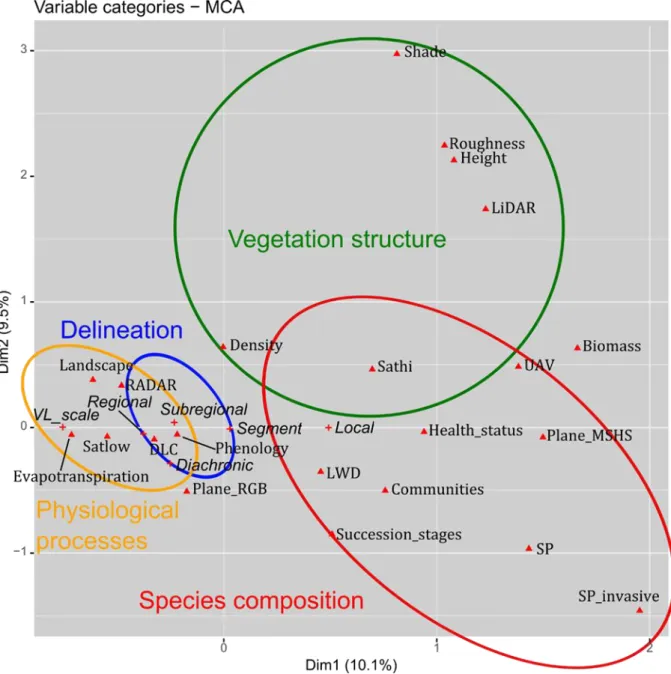
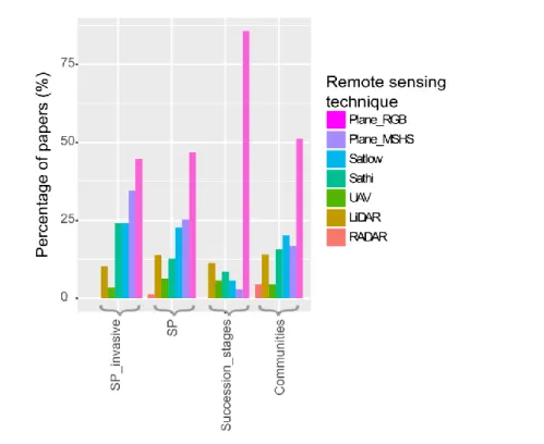
3.5. Which technology for which riparian feature?
330The features of interest extracted from remote sensing data to describe riparian vegetation were 331
strongly related to the type of remote sensing data (Figure 8). Four major trends emerged. First, the 332
study of physiological processes (e.g. phenology, evapotranspiration and, to a lesser extent, health 333
status) was strongly associated with the use of medium-resolution satellite images and large study 334
extents. Second, the study of features or processes related to vegetation structure (shade, 335
roughness, height) was strongly associated with the use of LiDAR data. Third, the study of features 336
related to species composition was associated with the use of high-resolution multispectral images 337
(acquired from satellites, planes or UAVs) or RGB/GS aerial images (especially for successional stages) 338
and with small study extents. Fourth, the delineation of riparian vegetation was weakly associated 339
with the use of RGB/GS aerial images or medium-resolution satellite images. These four trends are 340
discussed in the following four sections. 341
22 342
Figure 8. Results of the multiple correspondence analysis (see section 2.3. for the methods). Supplementary variables (i.e.
343
variables related to study extent and multi-temporality) are represented as crosses with text in italics. The first two axes
344
explain 19.6% of total variance. Ellipses were drawn arbitrarily to simplify interpretation. See Table 1 for code definitions.
345
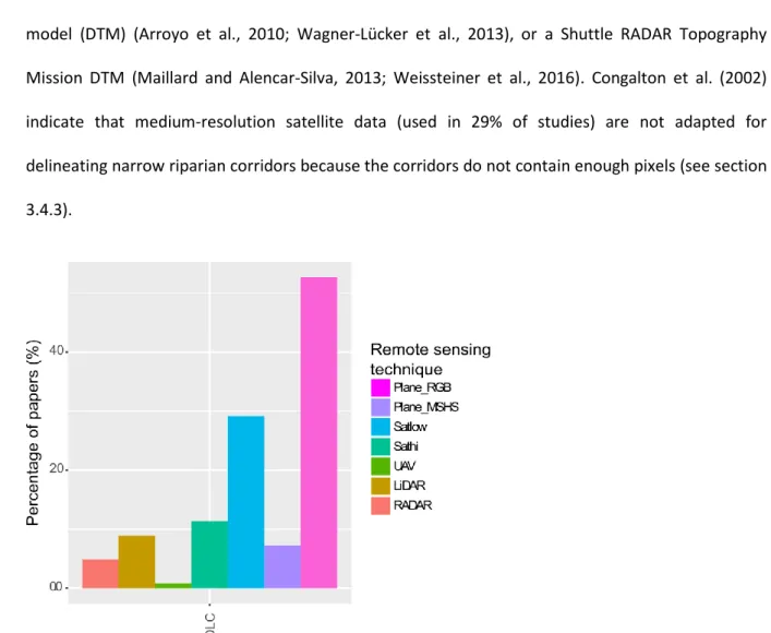
3.5.1. Delineation of riparian vegetation 346
How riparian vegetation is delineated depends on how it is defined (Verry et al., 2004). In general, 347
riparian vegetation is defined based on its specific characteristics (e.g. spectral signature, texture) 348
and on contextual information (e.g. topographic position, proximity to a river) (Weissteiner et al., 349
2016). Photointerpretation of RGB/GS aerial images is a traditional approach in which the operator 350
uses both types of information (Morgan et al., 2010). It was used in 53% of studies that delineated 351
23 riparian vegetation (Figure 9). Multispectral images (airborne or spaceborne, accounting for 45% of 352
studies) are often used to delineate riparian vegetation in an automated way (Alaibakhsh et al., 2017; 353
Johansen et al., 2010b; Bertoldi et al., 2011). Contextual information can be provided by ancillary 354
data (e.g. hydrographic network, as in Claggett et al. (2010) or Yang (2007)), a LiDAR digital terrain 355
model (DTM) (Arroyo et al., 2010; Wagner-Lücker et al., 2013), or a Shuttle RADAR Topography 356
Mission DTM (Maillard and Alencar-Silva, 2013; Weissteiner et al., 2016). Congalton et al. (2002) 357
indicate that medium-resolution satellite data (used in 29% of studies) are not adapted for 358
delineating narrow riparian corridors because the corridors do not contain enough pixels (see section 359
3.4.3). 360
361
Figure 9. Percentage of studies that used given remote sensing data to delineate riparian vegetation (i.e. distinguish riparian
362
vegetation from other land-cover types)
363
3.5.2. Species composition 364
Species composition is a recurrent subject that was studied in 42% of studies. Photointerpretation of 365
RGB/GS aerial images concerned 51%, 47% and 45% of studies that differentiated respectively 366
communities, species, and invasive species (Figure 7). This approach is widely used to describe 367
successional stages or changes in their distribution (86% of such studies). Indeed, RGB/GS aerial 368
images have been available since before the 1950s (González et al., 2010; Rood et al., 2010; Varga et 369
24 al., 2013; Wan et al., 2015). However, manual interpretation of images is time-consuming, and the 370
discriminating power of RGB/GS aerial images is limited by their low spectral range (Narumalani et 371
al., 2009; Fernandes et al., 2014). Medium-resolution satellite images were used in 21% of studies 372
that differentiated communities. These images were used mainly when vegetation patches were 373
larger than the image resolution (Vande Kamp et al., 2013; Hamandawana and Chanda, 2013; Sridhar 374
et al., 2010; Groeneveld and Watson, 2008; Townsend and Walsh, 2001), although spectral unmixing 375
can, to some extent, resolve this issue (Gong et al., 2015; Wang et al., 2013). 376
377
Figure 10. Percentage of studies that used given remote sensing data to map indicators related to species composition.
378
The most promising approaches to address this issue are based on high-resolution, aerial or 379
spaceborne, multispectral or hyperspectral images. These images were used in 30%, 33% and 45% of 380
studies that differentiated respectively communities, species and invasive species (Figure 10). The 381
accuracy of a particular project depends on the context, objectives, available data and methods used 382
to evaluate it. Therefore, we present recent studies that mapped species in the Table 2. In general, a 383
large number of narrow spectral bands increases the ability to distinguish species. However, in 384
mature, species-rich floodplain forests, it remains challenging to obtain classification accuracy that is 385
25 satisfactory for operational use, even when using hyperspectral imagery (Richter et al., 2016). The 386
use of multi-temporal images, which reveal the succession of phenological stages, can sometimes 387
replace the spectral range. For example, Rapinel et al. (2019) used Sentinel-2 time series to classify 388
grassland plant communities in a temperate floodplain using the relationship between inundation, 389
grassland management and vegetation composition. Similarly, Michez et al. (2016b) used UAV time 390
series to distinguish riparian tree species using images acquired during several phenological stages 391
(from spring to fall). It is also possible to acquire images at a single but appropriate date to take 392
advantage of the singular aspect of one species at a particular phenological stage. This approach is 393
especially effective when a single species has to be mapped, such as the invasive species Arundo 394
donax (Fernandes et al., 2013b) or Heracleum mantegazzianum (Michez et al., 2016a). The spatial 395
resolution of images must be sufficiently high to limit the occurrence of mixed pixels that hinder the 396
performance of automated classifications (Belluco et al., 2006; Narumalani et al., 2009). However, 397
small mixture of species remains a source of difficulty, even with a cm resolution (Michez et al., 398
2016a). LiDAR data, also used to classify species, can supplement multispectral data with vegetation 399
height data (Forzieri et al., 2013). They can also be used to segment trees before classifying them 400
(Dutta et al., 2017). They have also been used as the sole source of data by relating species identity 401
to the structure of the point cloud (Laslier et al., 2019). 402
26
Table 2. Examples of remote sensing methods used to classify riparian species in different settings and their accuracy
403
Reference Data Classes Accuracy Comment
Mature riparian forests Fernandes et
al. (2013a)
RGB-NIR aerial imagery (0.5 m resolution) 3 types of mature, temperate/Mediterranean riparian forests 61 (small) - 78% (large river) Dunford et al. (2009)
RGB imagery acquired with UAV (0.13 m resolution)
4 tree species (Populus, Salix and 2 Pinus) in a riparian Mediterranean forest 91% (for an image) - 71% (for a mosaic) Michez et al. (2016b)
RGB-NIR imagery acquired with UAV (0.1 m resolution)
5 tree species in a temperate, riparian forested/agricultural landscape 84 (forested) - 80% (agricultural) Multi-temporal dataset Richter et al. (2016)
Hyperspectral aerial imagery (367 bands, 2 m resolution)
10 tree species in a mature temperate floodplain forest
74% (single-date survey) - 78% (two-date survey) Dutta et al. (2017)
Hyperspectral aerial imagery (48 bands, 1 m resolution)
4 groups of tree species in a mature, temperate riparian forest
86% LiDAR is used to segment the trees
Laslier et al. (2019)
High density (> 45 points/m²) LiDAR point cloud
8 tree species in a temperate riparian agricultural/forested landscape
67%
Pionneer/species-poor riparian settings Macfarlane
et al. (2017)
Pansharpened GeoEye-1 imagery (RGB-NIR, 0.5 m resolution)
Pioneer (Salix, Populus) and invasive (Tamarix) species in an arid context
80%
Forzieri et al. (2013)
RGB-NIR aerial imagery (0.2 m resolution); hyperspectral aerial imagery (102 bands, 3 m resolution) and LiDAR data (DSM/DTM with 1 m resolution)
Pioneer (Salix, Populus) and invasive (Arundo donax) species in a temperate context
27
Invasive species Narumalani et al. (2009
Hyperspectral aerial imagery (62 bands, 1.5 m resolution)
Tamarix, Elaeagnus
angustifolia, Cirsium arvense, Carduus nutans and mixed
classes
74% Mixed classes are not well classified and decrease overall accuracy Fernandes et
al. (2014)
RGB-NIR aerial imagery (0.5 m resolution)
Arundo donax 97% Choice of the best date for aerial survey WorldView 2 imagery (8 bands, 2 m
resolution)
Arundo donax 95%
Michez et al. (2016a)
RGB-NIR imagery acquired with UAV (0.05-0.1 m resolution)
Impatiens glandulifera 72% Mixture with native species hinders accurate classification Heracleum mantegazzianum 97% Fallopia japonica 68% Peerbhay et al (2016)
WorldView 2 imagery (8 bands, 2 m resolution)
Solanum mauritanum 68%
Miao et al. (2011)
Hyperspectral aerial imagery (227 bands, 1 m resolution)
Prosopis glandulosa and Tamarix
92%
Doody et al. (2014)
WorldView 2 imagery (8 bands, 2 m resolution)
Salix 93%
These approaches based on high resolution data, although powerful, are mainly used at the local 404
scale. We showed in the section 3.4.2 that upscaling such data was challenging beyond a few dozen 405
km of river. However, at this scale, remote sensing would be a particularly useful alternative to field 406
campaigns or photointerpretation. Species classification methods that are more robust to upscaling 407
still need to be developed, as indicated by Fassnacht et al. (2016) in a review of forest tree species 408
classification. 409
3.5.3. Physiological processes 410
Medium-resolution satellite images (> 10 m resolution and ≤ 50 m for most studies) were the most 411
popular type of data used to assess physiological processes of riparian vegetation (100%, 73% and 412
28 54% of studies concerning respectively evapotranspiration, phenology and health status) (Figure 11). 413
One advantage of using these images in this context is that they are often available as dense series, 414
which is useful for studying cyclic processes. For example, Wallace et al. (2013) used AVHRR images 415
(return period < 1 day) to detect variations in the timing of greening up/scenescing of vegetation. 416
Nagler et al. (2012) used MODIS (return period 1-2 days) to study phases of the life cycle of the 417
tamarix leaf beetle (Diorhabda carinulata) throughout the year. Cadol and Wine (2017) and Nagler et 418
al. (2016) used long-term records (several years) of satellite images along with flow data to 419
investigate relationships between hydrology and physiological processes in riparian vegetation. 420
Zaimes et al. (2019) used a 27-year time series of Landsat images to study the impact of dam 421
construction on vegetation health status. Sims and Colloff (2012) used MODIS images over several 422
years to assess responses of riparian vegetation during and after flooding events. However, the low 423
resolution often means that pixels in the image aggregate greater heterogeneity in ground features. 424
Accuracy thus decreases, making it more complicated to study different types of vegetation 425
separately (Tillack et al., 2014; Cunningham et al., 2018). The health status of vegetation is often 426
studied with higher resolution data, occasionally with a single image (Tillack et al., 2014; Michez et 427
al., 2016b; Bucha and Slávik, 2013; Shendryk et al., 2016; Sankey et al., 2016). 428
429
Figure 11. Percentage of studies that used given remote sensing data to describe physiological indicators.
29 3.5.4. Vegetation structure
431
LiDAR appears to be the most used technology for describing vegetation structure features, except 432
for Large Woody Debris, landscape metrics and vegetation cover (Figure 12). LiDAR appears 433
therefore to be the most promising technology for describing vegetation structure and related 434
functions such as shading or surface roughness. The LiDAR signal can penetrate the canopy and the 435
water surface, and provides information about topography under dense canopies, the internal 436
structure of canopies and bathymetry. 437
438
Figure 12. Percentage of studies that used given remote sensing data to map structural features of riparian vegetation.
439
Retrieving simple structural attributes of vegetation (e.g. height, continuity, overhanging character) is 440
straightforward, since they can be extracted from DTMs, DSMs or CHMs delivered by LiDAR data 441
producers. These applications have reached an operational level. However, further methodological 442
developments for processing the 3D point cloud and new generations of full-waveform LiDAR data 443
must be explored before they can be transfered to management operations. For example, full-444
waveform LiDAR data have shown promising results in forestry applications (e.g. Koenig and Höfle, 445
2016), but there are few examples for riparian vegetation (Shendryk et al., 2016). 446
30 LiDAR data have been used in 90% of studies (Figure 12) to map riparian shade, which is a major 447
parameter that influences stream water temperature (Poole and Berman, 2001). Temperature 448
regulates the habitat of aquatic species such as the brown trout (Salmo trutta fario L.) (Caissie, 2006; 449
Georges et al., 2019), and the effect of riparian shade on stream water temperature is strong enough 450
to affect aquatic communities significantly (Bowler et al., 2012). Field methods used to measure 451
stream shade are expensive and time-consuming (Rutherford et al., 2018). LiDAR data appears to be 452
the most promising alternative because they can describe shade at a fine scale (Richardson et al., 453
2019). Several methods for using LiDAR data to measure riparian shade have been described in the 454
literature. Richardson et al. (2009) calculated light penetration index raster products as a predictor of 455
light conditions. LiDAR data can describe shadowing properties using a simple CHM derived from 456
point clouds (Michez et al., 2017; Loicq et al., 2018; Wawrzyniak et al., 2017). Other studies have 457
used 3D point clouds to retrieve the finest-scale information about vegetation structure. For 458
example, Akasaka et al. (2010) used a LiDAR point cloud to estimate biomass overhanging the river, 459
while Tompalski et al. (2017) used one to model solar shading on a given summer day. Recently, 460
Shendryk et al. (2016) used full-waveform LiDAR data to estimate the dieback of individual riparian 461
trees, which was related to their shadowing properties. 462
LiDAR data have also been used in 61% of studies to map floodplain roughness in a spatially 463
continuous manner (Figure 12). Forzieri et al. (2012) distinguished two main approaches for mapping 464
floodplain roughness using remote sensing: classification-derived mapping and hydrodynamic 465
modeling. In the former, thematic maps of land cover or vegetation classes are produced with 466
remote sensing data. A roughness coefficient (often Manning’s coefficient) is then assigned to each 467
class using a lookup table. In the latter, hydrodynamic properties of vegetation are estimated using 468
an indicator of vegetation structure (e.g. leaf area index, stem or crown diameter, vegetation height). 469
LiDAR technology has several advantages in this case: it measures structural attributes directly and 470
can account for complex, multilayered structures (Manners et al., 2013; Jalonen et al., 2015). 471
Hydrodynamic modeling is often combined with classification-derived mapping, with separate 472
31 modeling of hydrodynamic properties of each vegetation class (Straatsma and Baptist, 2008; Zahidi 473
et al., 2018). Development of restoration and multi-objective management practices (to promote 474
ecosystem health while protecting people and goods) has increased demand for models that 475
represent effects of vegetation on flow more accurately (Rubol et al., 2018). However, research on 476
hydrodynamic properties of vegetation and how to measure them in the field is ongoing (Shields et 477
al., 2017). 478
3.6. Multi-temporality of remote sensing riparian studies
479Overall, 54% of studies in the database were multi-temporal (i.e. studies where data acquired at 480
several dates are used to understand the dynamics of riparian vegetation). RGB/GS aerial images 481
were used in more than 60% of the multi-temporal studies (Figure 13A), such as those of Dufour et 482
al. (2015) or Lallias-Tacon et al. (2017). Such studies usually focus on decadal time scales. It can be 483
explained by the fact that this type of images is simple to use and has been available over a large 484
extent since the 1950s (Dufour et al., 2012). In most of the countries previously highlighted as active 485
in riparian research, public administrations have performed long-term and systematic national aerial 486
surveys for general purposes (e.g. urban planning) that researchers can use at low cost. Most multi-487
temporal studies that included aerial photographs used photointerpretation to describe riparian 488
vegetation features. Medium resolution satellite images were often used in multi-temporal studies, 489
notably for the study of physiological processes (see section 3.5.3). 490
32 491
Figure 13. Use of remote sensing data in (A) multi-temporal and (B) mono-temporal studies (respectively 54% and 46% of
492
the studies).
493
Conversely, more recent technologies (e.g. high-resolution satellite images, LiDAR data) were far 494
more common in studies that focused on one period than in multi-temporal studies (Figure 13B). For 495
example, LiDAR and high-resolution satellite data were used in respectively 24% and 18% of mono-496
temporal studies against 4% and 5% of multi-temporal studies. In mono-temporal studies, the 497
methods developed to map riparian forest attributes were more complex and mostly automated, 498
such as supervised classifications (Michez et al., 2016b; Antonarakis et al., 2008) and calculation of 499
metrics (Riedler et al., 2015). 500
We predict that diachronic analyses will be renewed by the increasing quality and availability of 501
remote sensing data. Indeed, data acquired from new sensors, such as LiDAR and hyperspectral 502
sensors, become more and more available as time series. For example, a LiDAR survey covers the 503
entire region of Wallonia (southern Belgium) every six years. In France, in the framework of the 504
Litto3D program, ca. 45,000 km² of coast (bathymetry included) will be regularly covered with a 505
dense LiDAR survey, in order to monitor sediment dynamics and erosion processes. These new data 506
provide the opportunity to monitor changes in specific features of riparian vegetation, such as 507
canopy height, species composition or fine scale physiological processes. In addition, acquisition 508
33 frequency has increased. For example, UAVs can acquire dense time series easily. High-resolution 509
satellite images such as Sentinel-1 and Sentinel-2 (four bands at 10 m resolution) provide images of 510
the Earth’s entire surface every few days. More recently, CubeSat constellations provide higher 511
resolution and higher frequency. For example, the Dove constellation (Planet Labs, Inc., San 512
Francisco, CA, USA) provides resolution up to 3 m and daily coverage. This increased frequency of 513
image acquisition provides new opportunities to study rapid riparian vegetation processes, including 514
intra-annual ones such as phenology and impacts of flood events. 515
4. Perspectives for riparian vegetation management
516
The second objective of this review was to discuss how remote sensing approaches developed by 517
scientists can be used by riparian managers. Research in remote sensing of riparian vegetation often 518
has an applied perspective, and 38% of the abstracts in our database contained the words 519
“management”, “restoration” or their derivatives. However, scientific articles usually do not describe 520
how remote sensing developments are made available to managers, and how they can be 521
implemented in management situations. 522
Therefore, we completed our systematic review of the literature with an approach based on expert 523
judgment, focusing on how remote sensing developments can be valued as operational tools 524
available to managers. In section 4.1, we selected five examples of applications for riparian 525
management. For each example, we highlight how remote sensing approaches can be embedded in 526
operational tools, and how scientific developments (previously discussed in section 3) can contribute 527
to these tools. In section 4.2, we further discuss the challenges of knowledge transfer from scientists 528
to managers, illustrated by the five selected examples. 529
4.1. Examples of near-operational applications
530We chose three contrasting fields of applications that we considered as particularly relevant for the 531
riparian context: eradication of invasive plant species, monitoring ecological integrity at the regional 532
scale and maintenance of hydraulic conveyance. 533
34 4.1.1. Example 1: Managing invasive plant species at the local scale
534
Riparian managers often conduct programs to eradicate invasive plant species. These programs 535
require identifying and locating individuals prior to eradication measures and subsequent monitoring 536
of invasive cover (i.e. to ensure that practices were effective and that the species do not re-emerge) 537
(Vaz et al., 2018). These actions can be perfomed with UAVs that combine high spatial resolution 538
(useful for detecting invasive plant species at an early stage, before they form large clumps) and high 539
temporal resolution (invasive plant species are often more distinct from the background during a 540
particular phenological phase, according to Manfreda et al. (2018)). Many studies have shown that 541
detecting invasive plant species using a UAV could outperform ground surveys in terms of cost, 542
effectiveness and risk mitigation for operators (Martin et al., 2018; Michez et al., 2016a). The 543
detection of invasive plants can be performed using photo-interpretation (most simple method) or a 544
supervised classification (most scalable method) of orthoimages (Hill et al., 2017). In the future, real-545
time or onboard processing (i.e. analysis of streamed imagery) will enable detection and eradication 546
steps to be performed at the same time (Hill and Babbar-Sebens, 2019). 547
In order to implement this approach, river managers must have access to skilled staff who are able to 548
pilot the UAV and process the images based on the needs of riparian managers. The staff can be 549
recruited and trained within the organization, or work for an exterior contracting organization. For 550
invasive species, work is often concentrated in time, and skilled staff must be available at that time. 551
4.1.2. Examples 2 and 3: Monitoring ecological integrity at the regional scale 552
Managers of riparian vegetation at the regional or national scale sometimes need information about 553
the entire river network to assess effects of policies or define management strategies (e.g. to 554
prioritize which zones should be restored). For example, all EU member states must monitor the 555
state of riparian ecosystems to comply with the Water Framework Directive (WFD), which promotes 556
a good health status of European rivers. These assessments have historically been performed during 557
field visits to sites sampled throughout each river network (Hering et al., 2010; Munné et al., 2003). 558
35 They can include remote sensing techniques in different ways. We briefly present two contrasting 559
approaches to include remote sensing in ecological assessments: a sampling- and 560
photointerpretation-based approach using aerial images, or the use of regional LiDAR data to map 561
riparian structural attributes automatically. 562
In the first approach (hereinafter referred to as example 2), aerial images can be integrated with 563
minor adaptations into a traditional field-based, sampling approach. Aerial images are used to target 564
sampling sites (e.g. where riparian vegetation is present) and to perform certain aspects of the 565
assessment, especially those that require less specific information at a larger scale. For example, the 566
Riparian Quality Index, initially developed for Iberian rivers, includes measurements of width, 567
continuity, strata, composition, regeneration, bank condition, lateral connectivity and substratum 568
(González del Tánago and García de Jalón, 2011). Width, continuity and strata can be described using 569
aerial imagery, while other attributes are assessed in the field. 570
In the second approach (hereinafter referred to as example 3), regional LiDAR data can be used to 571
assess riparian features in a spatially continuous manner. In this case, the strength of LiDAR data is 572
that the 3D component is homogenous at the regional scale unlike spectral data (see section 3.4.2). 573
Moreover, it can extract attributes of the channel even when it is hidden by vegetation. Riparian 574
attributes are calculated with a high level of automation and can be updated at the same frequency 575
as the actualization frequency of the LiDAR cover. For example, in Wallonia (southern Belgium), 576
Michez et al. (2017) used LiDAR and photogrammetric point clouds to map riparian buffer attributes 577
along 12,000 km of rivers (vegetation continuity, height and overhang; channel width and sinuosity; 578
and lateral connectivity, indicated by emerged channel depth). The results are meant to be used as 579
decision making tools by river managers. They are made available on an online platform, where river 580
managers must plan their management practices for a six year period. 581
4.1.3. Examples 4 and 5: Improving flood modeling with better estimates of 582
floodplain roughness 583
36 Many regions of the world must address significant and increasing threats of flooding, as well as the 584
need to conserve riparian ecosystems (Straatsma et al., 2019). Floodplain vegetation can influence 585
flood risk by increasing hydraulic roughness (Curran and Hession, 2013). In the Netherlands, where 586
these challenges are particularly acute, several remote sensing applications integrate riparian 587
vegetation management more into flood mitigation strategies. 588
One example (hereinafter referred to as example 4) includes a legal map produced to describe the 589
maximum roughness of vegetation cover allowed within the floodplains of major Dutch rivers. The 590
legal map uses a historical situation as a target reference (Rijkswaterstaat, 2014). To support use of 591
this legal map, Deltares (an independent applied research institute) and the Rijkswaterstaat (the 592
administration responsible for river management) developed an online vegetation-mapping tool 593
based on free multispectral, high-resolution satellite images. In the Google Earth Engine 594
environment, users can easily classify the vegetation cover observed on recent Sentinel-2 images to 595
ensure that it complies with the legal standard. The tool is available on smartphones and can be used 596
in the field. Actual vegetation can be compared to the map before each winter, when most floods 597
occur. The tool provides information about the areas on which management practices should focus, 598
following a dialogue with the landowners concerned (Penning, 2018). 599
Modeling approaches are also useful to support decisions. To prevent flood damage in Dutch deltas, 600
multiple practices, such as raising dikes or removing riparian vegetation, must be implemented in a 601
coordinated manner. Straatsma and Kleinhans (2018) developed the RiverScape toolbox. This tool 602
models the effects of riparian cutting on flow using hydrological and spatial data (including a DTM, a 603
vegetation map and its associated roughness coefficients). The RiverScape toolbox (hereinafter 604
referred to as example 5) can optimize the location of cutting operations to reduce water levels 605
during floods. 606
4.2. Challenges of conveying tools to managers
60737 The five examples given in the previous section illustrate that remote sensing approaches can be 608
embedded in operational tools for riparian managers. In this section, we discuss more generally how 609
scientists and managers can collaborate to produce and implement such tools for the management 610
of riparian vegetation. 611
We distinguish three main steps in this process (Figure 14). First, managers and remote sensing 612
experts must work together to define clear objectives. Second, the development step implies a 613
technological phase. Third, thorough assessment must be performed for accuracy, reliability and 614
relevance for managers. Critical thinking is required throughout this process because the choice of a 615
remote sensing approach is not neutral and has implications for how riparian vegetation is managed. 616
617
Figure 14. Conceptual framework of the transfer of remote sensing tools from scientists to managers. On the graphics to the
618
right, the horizontal axes represent scientific challenge and exchange degree to be planned between managers and
619
researchers (from low to high), while the vertical axes represent their dynamics from start to finish.
620
4.2.1. Identifying the issues/needs of riparian vegetation managers 621
The first step in implementing a remotely sensed application is to define the needs and objectives of 622
riparian vegetation managers. Key issues must be addressed, such as the features to be mapped, the 623
scale of observation, the time required to obtain usable information and the frequency of updating. 624
Objectives can be refined during the development step, depending on the tradeoffs between costs 625
and image quality. Nevertheless, thoroughly defining the objectives beforehand is clearly a factor of 626