Use of Sequential Estimation of Regressions and Effects on
Regressions to Solve Large Multitrait Test-Day Models
N. GENGLER,*, A. TIJANI, ,1 and G. R. WIGGANS *National Fund for Scientific Research, B-1000 Brussels, Belgium Animal Science Unit, Gembloux Agricultural University, B-5030 Gembloux, Belgium Animal Improvement Programs Laboratory, Agricultural Research Service, USDA, Beltsville, MD 20705-2350
Received July 22, 1999. Accepted January 7, 2000.
Corresponding author: G. Wiggans; e-mail: [email protected]. 1On leave from École Nationale d'Agriculture, Meknès, Morocco
2000 J. Dairy Sci. (Febr.)
Copyright 2000, the American Dairy Science Association. All rights reserved. Individuals may download, store, or print single copies solely for personal use. Do not share personal accounts or passwords for the purposes of disseminating this article.
ABSTRACT
An alternative algorithm for the solution of random regression models for analysis of test-day yield was developed to allow use of those models with extremely large data sets such as the US database for dairy records. Equations were solved in two iterative steps: 1) estimation or update of regression coefficients based on test-day yields for a given lactation and 2) estimation of fixed and random effects on those coefficients. Solutions were shown to be theoretically equivalent to traditional solutions for this class of random regression models. In addition to the relative simplicity of the proposed method, it allows several other techniques to be applied in the second step: 1) a canonical transformation to simplify computations (uncorrelated regressions) that could make use of recent advances in solution algorithms that allow missing values, 2) a
transformation to limit the number of regressions and to create variates with biological meanings such as lactation yield or persistency, 3) more complicated (co)variance structures than those usually considered in random regression models (e.g., additional random effects such as the interaction of herd and sire), and 4) accommodation of data from 305-d records when no test-day records are available. In a test computation with 176,495 test-day yields for milk, fat, and protein from 22,943 first-lactation Holstein cows, a canonical transformation was applied, and the biological variates of 305-d yield and persistency were estimated. After five rounds of iteration with a sequential solution scheme for the two-step algorithm, maximum relative differences from previous genetic solutions were <10% of corresponding genetic standard deviations; correlations of genetic regression solutions with solutions from traditional random regression were >0.98 for 305-d yield and >0.99 for persistency.
INTRODUCTION
Random regression models [e.g., (10)] that have been proposed for analysis of test-day yields (6) are computationally demanding, and few algorithms are available to simplify the computations. A (co)variance function can be defined as a continuous function that represents the variance and (co)variance of traits measured at different points on a trajectory (7, 8, 9). Recently, the
equivalence between random regression and (co)variance function models was shown (9, 13). Therefore, (co)variance function coefficients can be computed directly as (co)variance
components of the equivalent random regression model. The equivalence between random regression and (co)variance function models also can be used to simplify computations of random regression models (13).
The objective of this study was to develop an alternative algorithm to solve a random regression test-day model for use with extremely large data sets, such as the US national database of dairy records. Additional objectives were to facilitate the integration of data from 305-d records when no test-day records were available and to simplify the development of an index for lactation performance that includes genetic differences in lactation curve (persistency) and, for multiparity models, genetic effects of parity (maturity rate).
MATERIALS AND METHODS
Equivalence Between Random Regression and Infinite-Dimensional Models
Consider the following model to represent a special class of random regression modelsin which the same regressions are used for all time-dependent fixed and random effects:
where y = vector of observations (e.g., test days within traits within animal), b = vector of time-dependent fixed effects (e.g., herd test day), X = incidence matrix linking y and b, r = vector of time-independent random effects (e.g., phenotypic cow effects with several effects per animal that represent regression coefficients), Q = covariate matrix linking y and r and transforming time-dependent y to time-independent r, c = vector of time-independent fixed effects (e.g., age-season of calving), W = incidence matrix linking r and c, a = vector of random additive genetic effects, Z = incidence matrix linking r and a, p = vector of random nongenetic cow effects, and e = vector of residual effects (e.g., measurement errors).
The means and covariance structures of y, r, a, p, and e can be summarized as
[1]
where A = matrix of relationships among animals; R = variance-covariance matrix for e; I = identity matrix; KG and KP = genetic and environmental covariance matrices among random regression coefficients, respectively; and = Kronecker product operator.
This traditional random regression model also can be written to represent an infinite-dimensional model in which t = Qr:
For every animal i with records,
where t
i represents a vector of cow-specific effects that are observed for cow i.
The variance of ti then can be subdivided into genetic (Gi) and environmental (Pi) parts and modeled using covariance functions:
Therefore, the matrices K
G and KP are not only the genetic and environmental covariance matrices, respectively, among random regression coefficients but also the coefficients of the genetic and environmental covariance functions.
The regression covariate matrix Q is defined in general and can have different structures. The easiest way to understand this structure is through an example, such as the analysis of milk, fat,
y = Xb + t + e. [4]
yi = X
ib + ti + ei, [5]
and protein yields on first-lactation test days. Then,
where the test-day yields for milk, fat, and protein are ordered as observations within trait within animal so that Q can be split into Q
i blocks with a different block for each animal i. Each block is calculated as
where is defined as the matrix of regression variables associated with test-day yields for milk (m), fat (f), or protein (p) for animal i. The matrices for milk, fat, and protein can be different and may not be block diagonal; e.g., no protein yield was recorded, or more observations were recorded for milk than for component traits.
Alternative Two-Step Solution Algorithm
Solution of a random regression model traditionally is done through mixed model equations:
Because those equations are large and dense, their solution is difficult when the population to be analyzed is large. However, the mixed model equations can be subdivided into two sets of equations that can be solved sequentially. The first set of equations estimates b and p; the second estimates c and a.
[7]
[8]
Estimation of b and p (Step 1). At iteration k+1, the new estimate for b is obtained using current
estimates for c, a, and p as
which is derived from Equation [9]. Solutions can be computed directly herd by herd if fixed effects in b are defined specific to herd (e.g., herd test date). Block inversion also is possible, as the order of every block is limited and equal to the number of herd-specific levels in b.
The new estimate for p is obtained using current estimates for b, c, and a:
which also is derived from Equation [9]. An advantage of this approach is that solutions can be computed animal by animal because R is block diagonal for every animal. Therefore, direct inversion can be used in the computations (the order of the inverted block is equal to the number of regressions per animal).
The vector r is then updated using current estimates for c, a, and p:
Estimation of c and a (Step 2). Solutions for c and a in iteration round k+1 are obtained from
equations that are similar to regular multivariate mixed model equations:
Several solution techniques are possible because the secondary model is not completely specified. Canonical transformation can simplify computation (uncorrelated regression) by 1) transforming the multivariate equations in Equation [13] to several single-trait systems and 2) utilizing solution algorithms that allow missing values (1) as well as have other generalized uses as described by Ducrocq and Chapuis (2). Therefore, additional traits (such as lactation yield for cows without test-day records) also could be included. Variates with biological meaning (such as lactation yield, persistency, and maturity rate) could be created by transformation of regressions from Step 1 of the two-step algorithm. Such transformations would simplify the computations in Step 2 by limiting the number of traits (14), which then would facilitate the development of an index for lactation performance.
Other advantages result from splitting of random regression equations. Multiparity models can be developed by considering yields in second or later lactations to be additional traits. More complicated (co)variance structures than those usually considered in random regression models (e.g., additional random effects such as interaction of herd and sire) can be easily accommodated if (co)variance matrices for all random effects remain at least approximately diagonalizable in
[10]
[11]
[12]
Step 2 of the two-step algorithm.
Proof. To show that the solutions for b, c, and a from the two-step algorithm are equivalent to
those from Equation [9], first absorb p into the mixed model equations:
where M is the absorption matrix:
Based on Equation 9 and an equivalent model in which the effect of p appears only in the
residual covariance structure that is represented by M–1 (see Equation 15), the back solution for p gives
Use of Equation [16] is equivalent to the estimation of p as regression on test-day yields corrected for all other effects in the model. Next iterate on Equation [14] using two blocks:
Equations [16] and [17] are equivalent to estimating b and p in Equations [10] and [11] at k+1 rounds of iteration, and
Now the different blocks of the coefficient matrix in Equation [18] can be rewritten as
[14] [15] [16] [17] [18] [19] [20] [21]
After introducing those blocks, moving them to the right-hand side, and using the estimates of b at iteration k+1 and of c and a at iteration k,
Then
which shows that Equations [13] and [23] are equivalent because Equation [24] is the same equation as that obtained by including Equation [11], which updates p, in Equation [12], which updates r, and replacing M in Equation [15]. Therefore, solutions for c and a obtained from the two-step algorithm (Equation [13]) are equivalent to those from the mixed model equations (Equation [9]).
Similarity to the method of van der Werf et al. With cursory inspection, the two-step algorithm
does not appear to resemble the equations of van der Werf et al. (13). Their derivation was based on replacing y with a reduced form of the data, whereas the equations in the two-step algorithm (Equations [10], [11], [12], and [13]) were developed by subdividing a class of random
regression models into two models. However, the two-step algorithm can be shown to be a generalization of the van der Werf et al. (13) equations by restructuring the same equation that was used to demonstrate the equivalence between the solutions from the algorithm and the mixed model equations (Equation [24]):
That generalization of the expression of van der Werf et al. (13) includes time-dependent fixed effects, a general definition of R and Q, and no limitations on the covariance structures. Indirectly, the derivation of the two-step algorithm also is a proof of the equations of van der Werf et al. (13).
[22]
[23]
[24]
Sequential Solution Scheme
Similar to the approach proposed by van der Werf et al. (13), an expectation-maximization algorithm can be used to update r. During iteration, a part of r would be estimated once, and another part would be updated based on current estimates of b, c, and a:
where
In contrast to van der Werf et al. (13), who voluntarily avoided time-dependent fixed effects, the need also to update b leads to a sequential solution scheme that is based on Equations [10], [11],
[12], and [13] from the two-step algorithm. For most practical situations, solutions from a previous evaluation are available and can be used as starting values to speed up convergence, especially for fixed effects such as class of state, age, season, and lactation stage. For unknown herd test-day effects, a simple mean can be a good starting value. If genetic evaluations are calculated every 3 or 6 mo, the relative number of additional records compared with the total number of records would be at most 5 to 10%. For most animals, values for a and p are available, and pedigree values could replace estimates for a for new animals. Therefore, the following sequential solution scheme is possible:
1. Generate b using Equation [10] with starting values from a previous genetic evaluation. 2. Update r using Equation [12] after estimating p using Equation [11]. The solutions for b and p can also be obtained simultaneously through the following mixed model equations:
3. Solve for c and a using Equation [13] and starting values from the last genetic evaluation. 4. Update b using Equation [10] and the new estimates for c and a.
5. Solve for p using Equation [11] and the new estimates for b, c, and a, and update r using
Equation [12].
6. Update c and a using Equation [13].
7. Repeat from Step 4 until desired convergence is reached.
This scheme obviously only is equivalent to the traditional solution of a class of random regression equations if overall convergence can be achieved. The procedure is similar to the method proposed by Wiggans and Goddard (14). Such an approach also would be appropriate for advanced milk recording plans and continuous genetic evaluations. The estimations of b and r could be updated each time that data from a new test day are added for a given herd, thus
allowing their use for management purposes. The estimates of c and a could then be updated for the whole population on a scheduled basis (e.g., weekly, monthly, quarterly).
If cows change herds during lactation, estimation of b and p can become complicated because multiple incomplete lactations are created. Most current systems for genetic evaluation treat
[26]
multiple lactations as repetitions even though persistency differs for first and later lactations (e.g., 3). To extend sequential solution to multiple lactations, regressions would have to be linked to first and later lactations as different traits. Then only additional (incomplete) first or later (complete or incomplete) lactations would be treated as repetitions. Inclusion of an additional permanent environmental effect among lactations of a cow would allow effects that are specific to a cow but nongenetic to be applied from one lactation to the next, which would also address the difficulty of an incomplete lactation record.
Total overall convergence of the sequential solution scheme to approximate solutions from the two-step algorithm is not assured because of possible rounding errors and other problems linked to splitting the original mixed model equations (V. Ducrocq, 1998, personal communication). However, the two steps will converge separately, which allows the use of the two-step algorithm as a model that is approximately equivalent to a traditional random regression model. In
addition, attaining complete convergence for traditional random regression models often is difficult and slow (L. R. Schaeffer, 1999, personal communication).
Example Computations
Data. A total of 176,495 first-lactation test-day records for three yield traits (milk, fat, and
protein) that were recorded between 7 and 305 DIM were obtained for 22,943 Holstein cows that calved from 1990 through 1996 in large herds in Pennsylvania and Wisconsin. Test-day means were 28.1 kg for milk, 1.01 kg for fat, and 0.88 kg for protein; standard deviations were 6.8, 0.27, and 0.20 kg, respectively. Pedigree information for 43,342 animals was available from the Animal Improvement Programs Laboratory database. Groups of unknown parents were created based on birth years (<1981, 1981 to 1982, 1982 to 1983, ..., 1991 to 1992, >1992).
The model was based on Equation [1], but Xb was split into Hh and Ss, and third-order modified Legendre's polynomials (constant, linear, and quadratic) were used: I
0 = 1, I1 = 3
0.5x, and I 2 = (5/4)0.5(3x2 – 1), where x = –1 + 2[(DIM – 1)/(305 – 1)]. The resulting model was
where y = vector of test-day records for milk, fat, and protein yield; h = vector of effects for class of herd test day and milking frequency; s = vector of effects for class of state, age, season, and lactation stage; c = vector of nine fixed regression coefficients; a = vector of genetic random regression coefficients with nine coefficients per animal; p = vector of permanent environmental random regression coefficients with nine coefficients per cow with records; e = vector of residual effects; H, S, W, and Z = incidence matrices; and Q = covariate matrix for the third-order
Legendre's polynomials (constant, linear, and quadratic) for all traits (i.e., nine columns per animal). Assumed (co)variance structures were
y = Hh + Ss + Q(Wc + Za + p) + e [28]
where K
G = 9 x 9 covariance matrix of genetic random regressions (coefficients of the genetic covariance function); KP = 9 x 9 covariance matrix of permanent environmental random regressions (the coefficients of the permanent environmental covariance function); R0 = 3 x 3 residual covariance matrix among milk, fat, and protein test-day yields; A = additive genetic relationship matrix among animals; Ic = identity matrix of dimension c (number of cows or lactations); Ii = identity matrix of order equal to the number of known test days (no missing traits) for cow i; and = direct sum operator.
For this example, classes for state, age, season, and lactation stage were defined so that small classes would be avoided, but such classes should be smaller for actual calculation of genetic evaluations. Calving ages were 20 to 24, 25 to 26, 27 to 28, and 29 to 35 mo. Starting with January, six 2-mo calving seasons were defined. Twenty-two lactation stages based on DIM were defined: 7 to 13, 14 to 20, ..., 56 to 62, 63 to 76, 77 to 90, ..., 133 to 146, 147 to 167, 168 to 188, ..., 273 to 293, and 294 to 305 d.
The (co)variance components were based on those obtained previously by Gengler et al. (5) for similar data but adapted to three random regressions from the results reported by Tijani et al. (12).
Traditional solution for random regression model. Mixed model equations were based on
Equation [9]:
Those equations were solved with strategies for iteration on data that use a preconditioned conjugate gradient [e.g., (11)]. The convergence criterion was the relative squared difference between the right-hand sides and the left-hand sides times solutions.
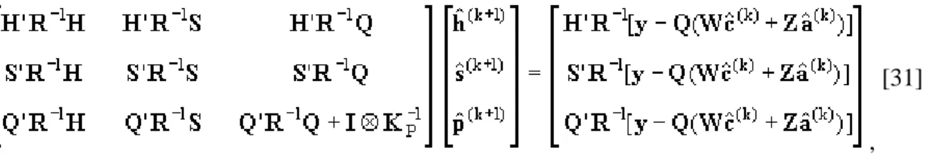
Sequential solution. Based on Equations [10] and [11] of the two-step algorithm modified to
include two fixed effects, the following system obtained from Equation [27] also was solved by using iteration on data and a preconditioned conjugate gradient:
and r was updated using Equation [12]. Because no information was available for c and a in the initial estimation of r, Equation [31] was modified in the first round of iteration to the following system:
which is equivalent to traditional estimation of r with a random regression model under the assumption that all cows are unrelated and that all the fixed regressions (c) are 0. Based on
Equation [13] of the two-step algorithm, c and a were estimated using canonical transformation and strategies for iteration on data that use second-order Jacobi iteration.
Estimation of 305-d yield and persistency. To illustrate the possibility of creating biologically
meaningful variates and to compare solutions from the traditional random regression model and the two-step algorithm, two new variates were calculated as linear functions of solutions for the three regressions: 305-d yield and persistency. The 305-d yield was defined as sum of all daily solutions from 1 through 305 DIM. Because persistency has been defined in different ways by various researchers (3), the method that has been used by the Canadian Dairy Network since February 1999 was chosen (6). This method is basically a linear function of the additive breeding value at 280 DIM minus the additive breeding value at 60 DIM.
RESULTS AND DISCUSSION
Data and model characteristics for the example computations are shown in Table 1. The
traditional random regression model (Equation [30]) produced 610,056 highly dense equations, especially because of the multiplication by 9 of the coefficients introduced by the A–1 matrices of animal relationships. With the two-step algorithm, the number of equations in Step 1 was
reduced to 219,897, and those equations also were less dense because no relationships among animals were included. The number of nonzero coefficients for animal equations was reduced, on average, from 81.5 (6 for fixed effects, 9 for fixed regressions, 9 x (1 + 5.39) for genetic effects, and 9 for permanent environmental effects) to 15 (6 for fixed effects and 9 for permanent environmental effects). Although relationships were included in Step 2 of the two-step
algorithm, the number of equations in Step 2 were reduced through canonical transformation to nine single-trait animal models.
, [31]
[32]
Solution of the traditional random regression model required 588 rounds of iteration to reach a convergence criterion value of 1 x 10⁻¹⁰. Because of concern about the convergence behavior of random regression models and because of a possible lack of convergence as indicated by some relatively large changes in solutions after further iteration, an additional 1000 rounds of iteration were computed. Convergence improved only to a value of approximately 1 x 10–11, but genetic regression solutions changed dramatically (up to 72% of a genetic standard deviation).
Therefore, computer word size was increased to 8 bytes to reduce rounding errors, and an additional 600 rounds of iteration were computed. This further iteration resulted in convergence values that oscillated between 1 x 10–13 and 1 x 10–14, and solutions for random regression effects changed up to a maximum of 12% of a genetic standard deviation. Those solutions were
considered to be reference solutions for comparison with solutions from the sequential solution scheme for the two-step algorithm even though convergence of the traditional random regression model might have been incomplete.
to solve alternative regression models based on test-day yield.
Category Number
Cows 22,943
Test-day yields1 529,485
Classes for herd test day and milking frequency2 10,242 Classes for state, age, season, and lactation stage3 3168 Inverse of relationship matrix
Animals 43,342
Genetic groups 8
Nonzero elements 276,970
Off-diagonals per line, 5.39
Equations
Traditional random regression model
(Equation [30]) 610,056 Two-step algorithm
Step 1 (Equations [31] and
[12]) 219,897
Step 2 (Equation [13]) 390,159
1Three yield traits, 176,495 test-day records. 2
Three yield traits, 3414 groups for herd test day and milking frequency.
3Three yield traits, two states, four calving age groups, six calving seasons, and 22 lactation stages.
The number of rounds of iteration was not used as a comparison criterion between solution methods as the time required per iteration was extremely different among the solution systems (traditional random regression model and Steps 1 and 2 of the two-step algorithm). The time needed for a round of iteration for the two-step algorithm also was variable because of the extensive use of previous solutions as starting values. Four rounds of iteration for the two-step algorithm took approximately 3% of the time needed for the >2000 rounds of iteration that were computed to solve the traditional random regression model; additional rounds of iteration for the algorithm would be faster.
To study overall convergence of the sequential solution scheme for the two-step algorithm, the maximum absolute differences of genetic regression coefficients were expressed relative to the corresponding genetic standard deviations (Tables 2, 3, and 4). Maximum relative differences from traditional random regression decreased rapidly to <10% by round 4 of iteration and stabilized around 7% for all three yield traits. Maximum relative differences from the previous round of iteration decreased steadily, which indicated that solutions from the sequential solution scheme were converging. This criterion also could be used as the overall convergence criterion for the two-step algorithm.
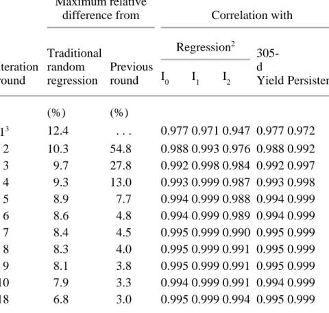
Table 2. Maximum relative differences1 and correlations between solutions for additive genetic regression coefficients for milk yield, estimated 305-d yield, and persistency obtained through random regression or sequential solution.
Iteration round
Maximum relative
difference from Correlation with
Traditional random regression Previous round Regression2 305-d Yield Persistency I0 I1 I2 (%) (%) 13 12.4 . . . 0.977 0.971 0.947 0.977 0.972 2 10.3 54.8 0.988 0.993 0.976 0.988 0.992 3 9.7 27.8 0.992 0.998 0.984 0.992 0.997 4 9.3 13.0 0.993 0.999 0.987 0.993 0.998 5 8.9 7.7 0.994 0.999 0.988 0.994 0.999 6 8.6 4.8 0.994 0.999 0.989 0.994 0.999 7 8.4 4.5 0.995 0.999 0.990 0.995 0.999 8 8.3 4.0 0.995 0.999 0.991 0.995 0.999 9 8.1 3.8 0.995 0.999 0.991 0.995 0.999 10 7.9 3.3 0.994 0.999 0.991 0.994 0.999 18 6.8 3.0 0.995 0.999 0.994 0.995 0.999
1Maximum absolute difference of additive genetic regression
coefficients expressed relative to the corresponding genetic standard deviations. 2I 0 = 1, I1 = 3 0.5x, and I 2 = (5/4) 0.5(3x2 – 1), where x = –1 + 2[(DIM – 1)/(305 – 1)]. 3
Initial computation was based on Equation [23].
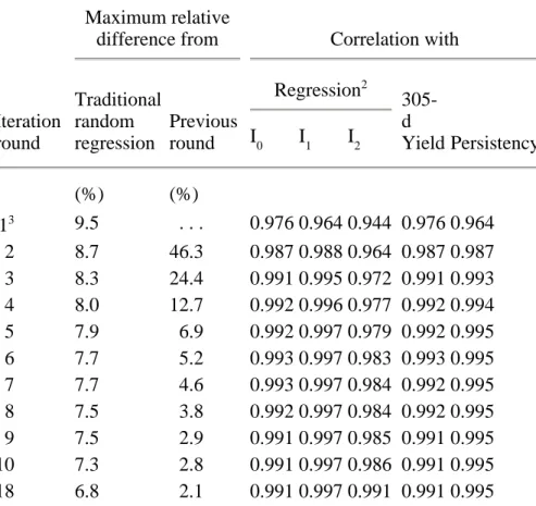
Table 3. Maximum relative differences1 and correlations between solutions for additive genetic regression coefficients for fat yield, estimated 305-d yield, and persistency obtained through random regression or sequential solution.
Iteration round
Maximum relative
difference from Correlation with
Traditional random regression Previous round Regression2 305-d Yield Persistency I0 I1 I2 (%) (%) 13 9.5 . . . 0.976 0.964 0.944 0.976 0.964 2 8.7 46.3 0.987 0.988 0.964 0.987 0.987 3 8.3 24.4 0.991 0.995 0.972 0.991 0.993 4 8.0 12.7 0.992 0.996 0.977 0.992 0.994 5 7.9 6.9 0.992 0.997 0.979 0.992 0.995 6 7.7 5.2 0.993 0.997 0.983 0.993 0.995 7 7.7 4.6 0.993 0.997 0.984 0.992 0.995 8 7.5 3.8 0.992 0.997 0.984 0.992 0.995 9 7.5 2.9 0.991 0.997 0.985 0.991 0.995 10 7.3 2.8 0.991 0.997 0.986 0.991 0.995 18 6.8 2.1 0.991 0.997 0.991 0.991 0.995 1
Maximum absolute difference of additive genetic regression
coefficients expressed relative to the corresponding genetic standard deviations. 2I 0 = 1, I1 = 3 0.5x, and I 2 = (5/4) 0.5(3x2 – 1), where x = –1 + 2[(DIM – 1)/(305 – 1)].
3Initial computation was based on Equation [23].
Table 4. Maximum relative differences1 and correlations between solutions for additive genetic regression coefficients for protein yield, estimated 305-d yield, and persistency obtained through random
Tables 2, 3, and 4 also show the correlations between additive genetic solutions for the three regressions, 305-d yield, and persistency from sequential solution of the two-step algorithm and those from traditional random regression. After the first round of iteration, which did not include relationships among animals or solutions for genetic effects, correlations for all yield traits were >0.93 for all regressions and >0.96 for 305-d yield and persistency. After an additional round of iteration, correlations for all traits were 0.98 for the constant and linear regressions (I0 and I1),
0.96 for the quadratic regression (I
2), and 0.98 for 305-d yield and persistency. After five rounds of iteration, correlations for all yield traits were 0.989 for I
0, 0.997 for I1, 0.976 for I2, 0.989 for 305-d yield, and 0.995 for persistency. In later rounds of iteration, correlations tended to plateau around 0.990 for I0, I2, and 305-d yield and around 0.995 for I1 and persistency.
regression or sequential solution.
Iteration round
Maximum relative
difference from Correlation with
Traditional random regression Previous round Regression2 305-d Yield Persistency I0 I1 I2 (%) (%) 13 11.6 . . . 0.964 0.978 0.931 0.964 0.977 2 10.5 57.0 0.980 0.994 0.960 0.980 0.994 3 10.0 30.4 0.985 0.998 0.969 0.985 0.998 4 9.6 12.4 0.987 0.999 0.973 0.987 0.998 5 9.3 7.6 0.989 0.999 0.976 0.989 0.999 6 9.1 5.7 0.989 0.999 0.978 0.989 0.999 7 8.9 6.3 0.990 0.999 0.980 0.990 0.999 8 8.7 4.1 0.990 0.999 0.982 0.990 0.999 9 8.5 3.7 0.990 0.999 0.983 0.990 0.999 10 8.3 3.5 0.989 0.999 0.984 0.989 0.999 18 7.3 3.0 0.990 0.999 0.989 0.990 0.999
1Maximum absolute difference of additive genetic regression
coefficients expressed relative to the corresponding genetic standard deviations.
2
I0 = 1, I1 = 30.5x, and I2 = (5/4)0.5(3x2 – 1), where x = –1 + 2[(DIM – 1)/(305 – 1)].
3
The plateaus in maximum relative differences and correlations between traditional random regression and sequential solution may be the result of several factors. The incomplete convergence of the random regression model is a primary consideration because sequential solution could be converging to a different value. In addition, sequential solution might be expected to provide more stable results than traditional random regression because the core of the sequential solution system is a canonical transformation algorithm, which would be expected to converge more rapidly because of its simpler (co)variance structure. Rounding errors during sequential solution also could explain some differences from random regression solutions. The correlations found in this study were slightly smaller than those reported recently by Gengler et al. (4) using a simplified version of the two-step approach: similar but fewer data, only one trait, and different variance components. After two rounds of iteration, they reported correlations of >0.98 with solutions from regular random regression.
CONCLUSIONS
Despite the similarity of the two-step algorithm and the method of van der Werf et al. (13), the derivations were based on different approaches. The two-step algorithm was developed by representing a phenotypic random regression model through a multitrait submodel on the phenotypic regressions, which was proved to be equivalent to a class of random regression models. However, as shown in the example computations, R from the two-step algorithm can describe much more complicated residual structures than can the diagonal matrix of van der Werf et al. (13).
Step 2 of the two-step algorithm simplified computations by allowing the use of canonical transformation and the transformation of regressions to create new variates for 305-d yield and persistency. Because missing values can be accommodated with canonical transformation (1), 305-d yield could be included for cows without test-day data. Another advantage of the two-step algorithm is the possibility for multiparity models.
Test computations showed that correlations of sequential solutions for milk, fat, and protein yields with solutions from traditional random regression were all >0.97 after five rounds of iteration even with incomplete sequential solution. Corresponding correlations were >0.98 for 305-d yield and >0.98 for persistency. The sequential solutions also showed overall convergence. The advantages of the proposed procedure for sequential estimation of regressions and effects on those regressions clearly outweigh any disadvantages from its only theoretical equivalence at overall convergence to traditional solution of mixed model equations of a class of random regression models. For those reasons and because of computational simplicity (including the use of parallelization in solving the system of equations), the sequential solution scheme allows application of random regression models to extremely large data sets. It could be a way to allow international test-day animal models in which Step 1 is done nationally and Step 2 is done internationnally.
ACKNOWLEDGMENTS
Brussels, Belgium, acknowledges its financial support. Aziz Tijani acknowledges the support of the Administration Générale de la Coopération au Développement, Brussels, Belgium. The authors thank Vincent Ducrocq, Institut National de la Recherche Agronomique, Jouy-en-Josas, France, for help in the development of the proof; Ignacy Misztal and Shogo Tsuruta, University of Georgia, Athens, for providing the random regression model solving program; and Paul VanRaden, Curt Van Tassell, Suzanne Hubbard, and Jill Philpot, Animal Improvement Programs Laboratory, ARS, USDA, Beltsville, MD, for manuscript review and HTML conversion. The authors also thank Ismo Stranden, Agricultural Research Centre, Jokioinen, Finland, and Julius van der Werf, University of New England, Armidale, New South Wales, Australia, for
manuscript review.
REFERENCES
1 Ducrocq, V., and B. Besbes. 1993. Solution of multiple trait models with missing data on some traits. J. Anim. Breed. Genet. 110:81–92.
2 Ducrocq, V., and H. Chapuis. 1997. Generalizing the use of the canonical transformation for the solution of multivariate mixed model equations. Genet. Sel. Evol. 29:205–224. 3 Gengler, N. 1996. Persistency of lactation yields: a review. Pages 87-96 in Proc. Int.
Workshop on Genet. Improvement of Functional Traits in Cattle, Gembloux, Belgium, January 1996. Int. Bull Eval. Serv. Bull. No. 12. Dep. Anim. Breed. Genet., SLU, Uppsala, Sweden.
4 Gengler, N., A. Tijani, and G. R. Wiggans. 1999. Iterative solution of random regression models by sequential estimation of regressions and effects on regressions. Pages 93-102 in Proc. Int. Workshop on Computational Cattle Breeding '99, Tuusula, Finland, March 18– 20, 1999. Int. Bull Eval. Serv. Bull. No. 20. Dep. Anim. Breed. Genet., SLU, Uppsala, Sweden.
5 Gengler, N., A. Tijani, G. R. Wiggans, C. P. Van Tassell, and J. C. Philpot. 1999. Estimation of (co)variances of test day yields for first lactation Holsteins in the United States. J. Dairy Sci. 82(Jan.). Online. Available: http://www.adsa.org. Accessed Dec. 15, 1999.
6 Jamrozik, J., L. R. Schaeffer, and J.C.M. Dekkers. 1997. Genetic evaluation of dairy cattle using test day yields and random regression model. J. Dairy Sci. 80:1217–1226.
7 Kirkpatrick, M., W. G. Hill, and R. Thompson. 1994. Estimating the (co)variance structure of traits during growth and aging, illustrated with lactation in dairy cattle. Genet. Res. Camb. 64:57–66.
8 Kirkpatrick, M., D. Lofsvold, and M. Bulmer, 1990. Analysis of the inheritance, selection and evolution of growth trajectories. Genetics 124:979–993.
9 Meyer, K., and W. G. Hill. 1997. Estimation of genetic and phenotypic (co)variance functions for longitudinal or "repeated" records by restricted maximum likelihood. Livest. Prod. Sci. 47:185–200.
10 Schaeffer, L. R., and J.C.M. Dekkers. 1994. Random regression in animal models for test-day production in dairy cattle. Proc. 5th World Congr. Genet. Appl. Livest. Prod., Guelph, ON, Canada VIII:443–446.
11 Shewchuk, J. R. 1994. An introduction to the conjugate gradient methods without the agonizing pain. Tech. Rep. CMU-CS-94-125. Carnegie Mellon Univ., Pittsburgh, PA.
12 Tijani, A., G. R. Wiggans, C. P. Van Tassell, J. C. Philpot, and N. Gengler. 1999. Use of (co)variance functions to describe (co)variances for test day yield. J. Dairy Sci. 82(Jan.). Online. Available: http://www.adsa.org. Accessed Dec. 15, 1999.
13 Van der Werf, J.H.J., M. E. Goddard, and K. Meyer. 1998. The use of covariance functions and random regressions for genetic evaluation of milk production based on test day records. 1998. J. Dairy Sci. 81:3300–3308.
14 Wiggans, G. R., and M. E. Goddard. 1997. A computationally feasible test day model for genetic evaluation of yield traits in the United States. J. Dairy Sci. 80:1795–1800.