The usefulness of outcrop-analogue air-permeameter measurements for analysing aquifer heterogeneity: testing outcrop hydrogeological parameters with independent borehole data

(1)

www.hydrol-earth-syst-sci.net/17/5155/2013/ doi:10.5194/hess-17-5155-2013

Hydrology and

Earth System

Sciences

The usefulness of outcrop-analogue air-permeameter measurements

for analysing aquifer heterogeneity: testing outcrop hydrogeological

parameters with independent borehole data

B. Rogiers1,2, K. Beerten1, T. Smeekens2, D. Mallants3, M. Gedeon1, M. Huysmans2,4, O. Batelaan2,4,5, and A. Dassargues2,6

1_{Institute for Environment, Health and Safety, Belgian Nuclear Research Centre (SCK·CEN), Boeretang 200,}

2400 Mol, Belgium

2_{Dept. of Earth and Environmental Sciences, KU Leuven, Celestijnenlaan 200e – bus 2410, 3001 Heverlee, Belgium} 3_{Groundwater Hydrology Program, CSIRO Land and Water, Waite Road – Gate 4, Glen Osmond, SA 5064, Australia} 4_{Dept. of Hydrology and Hydraulic Engineering, Vrije Universiteit Brussel, Pleinlaan 2, 1050 Brussels, Belgium} 5_{National Centre for Groundwater Research and Training (NCGRT), School of the Environment, Flinders University,}

G.P.O. Box 2100, Adelaide, SA 5001, Australia

6_{Hydrogeology and Environmental Geology, Dept. of Architecture, Geology, Environment and Civil Engineering (ArGEnCo)}

and Aquapole, Université de Liège, B.52/3 Sart-Tilman, 4000 Liège, Belgium

Correspondence to: B. Rogiers (brogiers@sckcen.be)

Received: 28 June 2013 – Published in Hydrol. Earth Syst. Sci. Discuss.: 23 July 2013 Revised: 17 October 2013 – Accepted: 18 November 2013 – Published: 18 December 2013

Abstract. Outcropping sediments can be used as easily

ac-cessible analogues for studying subsurface sediments, espe-cially to determine the small-scale spatial variability of hy-drogeological parameters. The use of cost-effective in situ measurement techniques potentially makes the study of out-crop sediments even more attractive. We investigate to what degree air-permeameter measurements on outcrops of uncon-solidated sediments can be a proxy for aquifer saturated hy-draulic conductivity (K) heterogeneity. The Neogene aquifer in northern Belgium, known as a major groundwater re-source, is used as the case study. K and grain-size data ob-tained from different outcropping sediments are compared with K and grain-size data from aquifer sediments obtained either via laboratory analyses on undisturbed borehole cores (K and grain size) or via large-scale pumping tests (K only). This comparison shows a pronounced and systematic differ-ence between outcrop and aquifer sediments. Part of this dif-ference is attributed to grain-size variations and earth surface processes specific to outcrop environments, including root growth, bioturbation, and weathering. Moreover, palaeoen-vironmental conditions such as freezing–drying cycles and differential compaction histories will further alter the initial

hydrogeological properties of the outcrop sediments. A lin-ear correction is developed for rescaling the outcrop data to the subsurface data. The spatial structure pertaining to out-crops complements that obtained from the borehole cores in several cases. The higher spatial resolution of the out-crop measurements identifies small-scale spatial structures that remain undetected in the lower resolution borehole data. Insights in stratigraphic and K heterogeneity obtained from outcrop sediments improve developing conceptual models of groundwater flow and transport.

1 Introduction

Compared to core drilling for sample collection and analysis, outcropping sediments are easily accessible analogues for studying subsurface sediments. This outcrop-analogue con-cept has been extensively applied in the oil industry for the analysis and modelling of reservoirs (e.g. Flint and Bryant, 1993; McKinley et al., 2004) resulting in various tools to characterize geological facies geometries, their connectivity and continuity (Pringle et al., 2004), and to create 3-D virtual

(2)

a very limited number of facies are generally encountered in a single outcrop. The information contained within such lithofacies type potentially represents key stratigraphic fea-tures and hydrogeological parameters for building concep-tual groundwater flow models. Furthermore, different out-crops may represent different parts of a stratigraphic or land-scape succession series (Beerten et al., 2012). The combina-tion of several outcrops can then be used to obtain a com-posite picture of an aquifer system containing the same or at least similar sediments. As demonstrated by Rogiers et al. (2013a), the use of a hand-held air permeameter is a very accurate and cost-effective approach for quantifying hy-draulic conductivity (K) and its spatial variability in situ on outcropping sediments. The question that remains however is how representative the obtained outcrop parameters are for the actual subsurface sediments.

In first instance, the outcrop sediments may differ in some aspects from their subsurface equivalents as a result of slightly differing depositional contexts, e.g. with respect to the position in the basin (palaeogeographical conditions). Inherently, this problem is largely circumvented by compar-ing outcrop and subcrop sediments from one and the same formation.

Secondly, the outcropping sediments could also be influ-enced by post-depositional processes such as surficial weath-ering and compaction due to slightly different overburden sedimentation and erosion histories. During the initial load-ing of sands, a rapid increase of packload-ing density and soil strength is expected due to grain reorganization (Pettersen, 2007). As packing becomes tighter, further packing will be increasingly more difficult to achieve, each packing level is more stable than previous levels and deformation is perma-nent. This process should be visible in the porosity, bulk den-sity and eventually K data of a progressively compacted ma-terial. Overconsolidated sands should however not show di-lation properties, and unloading would thus have little effect. However, the amounts of silt and clay present throughout the aquifer sediments might initiate such dilation properties. Moreover, dissolution of certain mineral phases or frame-work grains by meteoric water might also enhance perme-ability, as shown by Lambert et al. (1997).

The objectives of this paper are therefore (i) to test whether the hydraulic conductivity and its spatial heterogeneity in outcrops obtained through air permeametry are comparable to those of nearby aquifer and aquitard sediments, (ii) to

the observed differences in K behaviour and options on how to integrate air permeametry-based data with existing knowl-edge available from borehole and pump test analyses in view of developing more reliable groundwater flow models.

2 Materials and methods

Table 1 provides an overview of all data used in this paper. The hydrogeological setting and the outcrop measurements are discussed first. The data at each outcrop has been up-scaled to an equivalent K tensor. Next, the constant-head measurements on the borehole core samples are discussed. The procedure for obtaining grain-size distributions is de-scribed, and we shortly introduce the used pumping test methods and analyses. Finally we outline the approach for variography of the data to quantify spatial variability.

2.1 Hydrogeological setting and outcrop analyses

Rogiers et al. (2013a) proposed a methodology to measure small-scale K variability from unconsolidated outcrop sed-iments and to calculate outcrop-scale equivalent K values. This methodology relies on air permeability measurements that are converted to saturated K values using the empirical equation from Iversen et al. (2003), and a subsequent numer-ical upscaling step. The air permeability measurements are performed with a hand-held air permeameter, the Tinyperm II (New England Research & Vindum Engineering, 2011), on a regular grid of measurement locations at the outcrop face. The TinyPerm II device has an inner tip diameter of 9 mm, resulting in an investigation depth of 9–18 mm, correspond-ing to a maximum spatial support of ∼ 24 cm3. Pressing the device plunger will create a vacuum to withdraw air from the outcrop sediments. A microprocessor analyzes the pressure increase, and returns air permeability. The resulting values cannot be converted directly to saturated hydraulic conduc-tivity because corrections are needed in regards to (i) the po-lar characteristics of water, (ii) the fact that air at atmospheric pressure does not act as a true fluid continuum in soil (e.g. gas slippage might occur at the interface with solids), and (iii) the difficulty in obtaining totally dry conditions in the investi-gated sediments. The use of empirical relationships like that of Iversen et al. (2003) has proven to be very effective in converting air permeability into hydraulic conductivity.

(3)

Table 1. Overview of the different K and grain-size samples used in this paper.

Sediment Parameter Outcrop Borehole Pumping

test

Mol formation

No. of K samples 32 161 9

No. of grain-size measurements – 61 –

Sample spacing 20 cm 2 m –

Measurement support ∼24 cm3 100 cm3 large-scale

Kasterlee formation: sandy part

No. of grain-size measurements 6 12 –

Kasterlee formation: clayey part

Diest formation: clayey part

No. of K samples 192 89 –

Diest formation: sandy part

No. of grain-size measurements – 42 –

Measurement support ∼24 cm3 100 cm3 large-scale Source: Rogiers et al. (2013a) and Beerten et al. (2010).

This methodology was tested on five outcrops from three key formations of the Neogene aquifer in north-eastern Bel-gium (from top to bottom): the Mol formation (the abbrevi-ation Fm. will be used in the subsequent discussions), sandy and clayey parts of the Kasterlee Fm., and the clayey and sandy parts of the Diest Fm. For these five formations addi-tional geological and hydrogeological data is available from a recent characterization campaign (Beerten et al. 2010) of the shallow aquifer sediments in Mol/Dessel (up to about 40 m depth), including seven cored boreholes (Fig. 2 in Rogiers et al., 2013a). This lithostratigraphical succession and its main characteristics are presented in Fig. 1. Apart from the minimum and maximum unit thickness obtained from this recent characterization campaign, a typical bore-hole core from the clayey Kasterlee Fm. is displayed, as well as a grain-size and glauconite content profile through most of the units. The most striking features are the high clay and fine silt contents within the aquitard represented by the clayey part of the Kasterlee Fm., the sudden increase of the glauconite content in the sediments below this unit, and the contrast in coarse sand content between the upper and lower aquifers separated by the aquitard.

In addition to the individual air-permeameter measure-ments (spatial support of ∼ 24 cm3) and their statistics, the measurement grids were numerically upscaled to ob-tain equivalent horizontal and vertical K values at the scale

Minimum thickness Maximum thickness ≈ 2 m ≈ 10 m ≈ 2 m ≈ 5 m ≈ 7 m ≈ 5 m ≈ 20 m ≈ 6 m ≈ 7 m ≈ 10 m 1 m Typical glauconite content % wt 0 20 40 60 Typical grain-size profile % wt 0 50 100 Q M SK CK CD Q M SK CK CD

Fig. 1. Overview of the studied lithostratigraphical succession with

formation thicknesses, typical glauconite content (weight percent-age; % wt), and a typical grain-size profile. A picture of a borehole core from the clayey part of the Kasterlee formation is provided to illustrate its heterogeneity. For more information, see Beerten et al. (2010).

of the outcrop (i.e. typically several m2; Rogiers et al., 2013a). This was done by using the approach of Li et al. (2011). The measurements on the sampling grid were con-verted into a numerical grid, with one extra grid cell at all sides. By invoking flow conservation for a combination of

(4)

Fig. 2. Cumulative grain-size distributions for the outcrop (laser diffraction) and borehole data (mean value and 5–95 percentiles from

SediGraph or standard method; Beerten et al. 2010) for (A) the sandy Kasterlee Fm., (B) the clayey Kasterlee Fm. and (C) clayey Diest Fm.

different boundary conditions an equivalent K tensor was obtained. An overview of this approach for all outcrops characterized by air-permeameter measurements within the study area is provided by Rogiers et al. (2013b). The in-dividual small-scale air-permeameter results show a corre-lation of 0.93 with independent constant-head laboratory permeameter measurements on 100 cm3ring samples taken from the same outcrop measurement grid (Rogiers et al., 2013a). The average ratio between both log-transformed K data (air permeameter/constant head) equals 1.03, and is be-tween 0.78 and 1.24 for individual samples. Repeatability of the TinyPerm II measurements was tested on a set of differ-ent lithologies with K ranging from 10−3.5 _{to 10}−6.5_{m s}−1_,

with maximum log₁₀(K)error variance of 0.007. Given this high repeatability, and the absence of visible macropores in the investigated outcrop faces, the K data obtained from the outcrops is deemed accurate and unbiased.

2.2 Constant-head K measurements

To characterize the aquifer sediments’ hydraulic conductivity variability, multiple undisturbed 100 cm3ring samples (with diameter of 53 mm) were taken from contiguous borehole cores (Beerten et al., 2010). The ring samples were pushed in the cores in horizontal or vertical direction, for characteri-zation of respectively horizontal or vertical K. The gathered data enclose several hundred hydraulic conductivity mea-surements on such 100 cm3 _{ring samples from seven cored}

boreholes, representing 350 m of core material. Two sam-ples were taken each 2 m, for horizontal and vertical K, but the anisotropy at the sample scale was generally negligible (Beerten et al., 2010). The average thickness of the Mol and Kasterlee formations in these boreholes is respectively 20 and 10 m. The highly stratified clayey part of the Kaster-lee Fm. – coarse sand layers alternate with heavy clay lenses with thickness varying from less than a cm to several cm – varies in thickness from 2 to 6 m. The Diest formation is not penetrated fully, but was characterized on average across 15 m.

All 100 cm3 ring samples were analyzed in the lab us-ing the constant-head method (Klute, 1965), usus-ing a low-pressure device for coarse material and a high-low-pressure de-vice (approx. 6 bar) for the clay material expected to display low K values (see Beerten et al., 2010 for more details). To-tal porosity was also determined for most core samples, as well as bulk density and volumetric moisture content for the outcrop samples, by repeatedly weighing the samples after drying and complete saturation. The methodology is similar to that used by Rogiers et al. (2013a) to validate the outcrop air-permeameter measurements.

2.3 Grain-size measurements

A SediGraph or a combination of standard sieving and a sus-pension cylinder (European standard EN 933-1) was used to quantify, respectively, 20 and eight grain-size fractions of the borehole core samples. All samples were prepared by remov-ing carbonates and organic matter. Clay samples were an-alyzed with the SediGraph, after removing particles larger than 250 µm by sieving. For more details on the data, the reader is referred to Beerten et al. (2010) and Rogiers et al. (2012).

Grain-size analyses of outcrop samples were performed by laser diffraction with a Malvern Mastersizer (Malvern Instruments Ltd., UK). This method consists of monitoring the amount of reflection and diffraction that is transmitted back from a laser beam directed at the particles, and quan-tifies 64 grain-size fractions. Each sample was divided into 10 sub-samples by a rotary sample splitter to enable repeated measurements on a single sample, and all samples were mea-sured at least twice. The final result was based on the average grain-size distribution of all sub-samples. Note that particle sizes are expressed as the size of an equivalent sphere with an identical diffraction pattern.

2.4 Pumping tests

Step drawdown, constant discharge and recovery tests were performed at different locations within the study area, including some of the borehole locations. The transient

(5)

groundwater head observations were interpreted with analyt-ical as well as numeranalyt-ical models (Meyus and Helsen, 2012). Results from these large-scale tests are used here to illustrate the scale effect for hydraulic conductivity determination on subsurface sediments, and to compare such large-scale mea-surements with the numerically upscaled K values for the outcrops.

2.5 Variography

The experimental variograms are all fitted with spherical models, using a weighted least squares approach. Two ap-proaches are tested: (1) treating both data sets separately (variogram models for the outcrops are taken from Rogiers et al., 2013a), and (2) using a pooled data set which com-bines both outcrop and borehole data. In the latter case equal weight is given to both data sets in the least squares fitting. In the former case individual experimental variogram points are weighted according to the number of point pairs they rep-resent. The initial variogram parameters for the nugget, to-tal sill and range were respectively set to the overall min-imum semivariance, the data variance, and the maxmin-imum lag distance. In certain cases singular model fits occurred due to non-uniqueness (data does not allow to discriminate between different equivalent models, e.g. pure nugget vs spherical model with zero range). The responsible parame-ters were then fixed at their initial value, before re-initialising the model fitting procedures. All variography was performed with the gstat package (Pebesma, 2004).

3 Results and discussion 3.1 Grain-size distributions

Prior to comparing K values obtained from different mea-surement methods, a comparison is made between grain-size distributions for the outcrop sediments and aquifer materials collected from cored boreholes (Beerten et al., 2010). This evaluation is necessary to verify if the outcrop and aquifer sediments represent the same lithostratigraphical units, and to highlight possible discrepancies between both to inform the comparison of their corresponding K values.

Overall there is good correspondence between out-crop/aquifer grain-size distributions for the sandy part of the Kasterlee Fm. and clayey part of the Diest Fm. (Fig. 2a– c), with a somewhat larger fraction of fines (i.e. between 2 and 22 µm) for the outcrop samples. Van Ranst and De Coninck (1983) suggested that post-depositional weathering of glauconite material, a green iron-rich clay mineral, might increase the relative amount of fines. Kasterlee formation samples collected from boreholes contain glauconite up to a few percent, but for the Diest formation it is at least 10 to 20 % (Beerten et al., 2010). The disintegration of the glau-conite fractions in the outcrops could thus have increased the fines content.

The comparison further illustrates that the clay fraction (< 2 µm) of the clayey part of the Kasterlee Fm. is about 20 % lower in the outcrop samples compared to the aquifer material. Since we are dealing with outcrop samples that are close to the surface, post-depositional migration of clay out of the clay lenses (e.g. Mažvila et al., 2008) together with bioturbation in the outcrops is a plausible explanation for the lower clay content in the outcrop. Weathering of clay lenses or drapes close to the surface would be another plausible ex-planation. For the clayey Kasterlee Fm. outcrop, the individ-ual grain-size distribution curves (Fig. 2b) indicate a contin-uous gradation between two extreme cases, i.e. from a clay lens texture (approximately 40 % clay) to coarse sand with-out fines (> 90 % sand). The corresponding grain-size distri-butions for boreholes show no overlap between the clay and sand samples, an illustration of the existence of two distinctly different materials within the clayey part of the Kasterlee Fm. (i.e. heavy clay lenses embedded in coarse sands character-ized by a sharp interface) (Beerten et al., 2010).

In conclusion, weathering, clay migration, and biotur-bation may have influenced the lower end of the outcrop samples’ grain-size distribution considerably. Furthermore, dissimilarities in palaeogeographic conditions and sediment source regions between the outcrop and borehole locations may equally explain such differences. However, the consis-tent stratigraphic position of the clayey Kasterlee Fm. sedi-ments on top of the Diest Fm. and the relatively good corre-spondence in particle size for the sandy material (i.e. sand layers within the Kasterlee Fm.), are sufficient underpin-ning arguments to support using the studied clayey Kasterlee Fm. outcrop at Heist-op-den-berg (for details of the outcrop see Rogiers et al., 2013a) as surrogate for the clayey Kaster-lee Fm. aquitard (Gulinck, 1963; Laga, 1973; Fobe, 1995). Additional insight could be obtained from tracing the exact origin and initial composition of the outcrop materials; how-ever, this is beyond the scope of the current paper.

3.2 Hydraulic conductivity distributions

Figure 3 provides a comparison of outcrop and borehole (aquifer) K kernel density estimates of the probability den-sity functions (pdfs) for the five sediments. Statistically sig-nificant differences exist for all sediments, with p values for

F tests all below 4 × 10−3, while the corresponding t tests

p values are all below 1 × 10−5indicating statistically sig-nificant differences for both the variance and mean. All out-crop pdfs have higher mean K values than their borehole complement. While most outcrop samples display conductiv-ities between 10−5 and 10−3m s−1, borehole samples have their most frequent K values between 10−6and 10−4m s−1. Moreover, the standard deviations for the borehole samples are consistently larger than those based on the outcrop sam-ples. The left tail of the pdfs tends to be much larger for the borehole data while the peaks tend to be wider (one to two or-ders of magnitude for the outcrops versus two to four oror-ders

(6)

Fig. 3. Comparison between distributions (kernel density estimates of the probability density functions) for air-permeameter-based outcrop Kand constant-head K measurements on undisturbed samples from cored boreholes, for (A) the Mol Fm., (B) the sandy Kasterlee Fm.,

(C) the clayey Kasterlee Fm., (D) the clayey Diest Fm. and (E) the sandy Diest Fm. Mean (µ) and standard deviation (σ ) are given for both

data sources.

of magnitude for the borehole data), especially for the sandy Kasterlee Fm. (Fig. 3b). Relative variability expressed as co-efficient of variation (CV) is approximately two times larger for borehole pdfs than for outcrop pdfs (Mol Fm.: −13.4 % vs −5.9 %; Kasterlee Fm. sands: −24.5 % vs −12.9 %; Di-est Fm. sands: −23.9 % vs −18.8 %) while it is similar for the clayey parts of the Kasterlee Fm. (−23.9 % vs −18.8 %) and Diest Fm. (−15.8 % vs −17.4 %). For the borehole data, sampling occurred over a large geographical area (several tens of km2 vs as little as a few m2 to at most a few tens of m2for the outcrops) and over a much larger depth (up to 50 m) thus having the opportunity to sample a much larger spatial heterogeneity.

Several characteristics typical of heterogeneity in K are however visible in both the outcrop and borehole K distri-butions. For the sandy part of the Kasterlee Fm. (Fig. 3b), a long tail towards low values is present both in the outcrop and in the boreholes, while the majority of samples is within a much narrower distribution in the outcrop. For the clayey part of the Kasterlee Fm. (Fig. 3c), a multi-modal distribution is present for both data sets and representative of samples be-longing mainly to clay lenses or sand layers. The clayey part of the Diest Fm. (Fig. 3d) displays a similar pdf in both data sets (ratio of borehole to outcrop CV = 0.91), and the sandy Diest Fm. data (Fig. 3e) shows the best absolute match in terms of the mean K, although the second peak with lower

Kvalues was not observed in the outcrop.

Validation of air permeameter K with core-based out-crop K demonstrated absence of systematic bias in the air-permeameter K estimates (Rogiers et al., 2013a). Therefore, differences in K distributions between outcrop and aquifer sediments can be attributed to the scale of investigation (a

single outcrop with a typical measurement grid of a few m2 vs seven ∼ 50 m-deep vertical transects through the different lithostratigraphical formations, Fig. 1), different evolution-ary states of the outcropping and subsurface sediments, and possibly different sedimentation conditions.

3.3 Linear rescaling correction

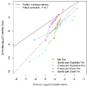
To investigate the (dis)similarities between the outcrop and borehole data across these five lithological units, the min-imum and maxmin-imum values are plotted in Fig. 4, with all deciles (10th, 20th, . . . , 90th percentile) in between. This shows that linear scaling of the outcrop values to the corre-sponding borehole distributions is possible for all outcrops. The extreme values are however not always in line with the centre of the distributions (as indicated by the deviation of the overall shape of the first and last line segments). All outcrops exhibit a more or less similar trend for at least part of the data, which is supported by the linear model fit on all minimum, maximum and decile points (r2= 0.7). The slope, larger than 45◦, indicates that the deviation between outcrop and bore-holes is larger for low K than for higher K values, which is consistent with the previous observations. The sandy Di-est Fm. curve lies apart and above the other curves, and is much closer to the 1 : 1 line of perfect agreement. This is as expected based on the good correspondence in pdfs (see Fig. 3e). In other words, the Diest Fm. outcrop is well and truly representative for the entire aquifer unit.

3.4 Porosity and compaction state

Weathering of clay layers at the surface has certainly con-tributed to produce higher K values for the fine material

(7)

Fig. 4. Outcrops versus borehole log₁₀(K)deciles, and a fitted lin-ear correction model (y = 0.6938 + 1.5685 x).

in the outcrops, but the systematic bias of about one or-der of magnitude that is also present for the sands remains unexplained.

Trends in porosity or bulk density with depth are very hard to detect in the borehole data due to the extensive layering of different lithologies and grain-size distributions at the study area (the same lithology may occur at different depth depend-ing on the geographical location). Moreover, the data from the outcrops are hardly sufficient to prove differences with the subsurface sediments are statistically significant. For ex-ample, the mean total porosity for the four Mol and Kaster-lee Fm. outcrop core samples is 43 % with a mean dry bulk density of 1.52 g cm3 (see Rogiers et al., 2013a), while the borehole values of the same two formations (43 samples) are 40 % and 1.60 g cm−3 (samples between 2 and 28 m below surface). This is consistent with different compaction states (i.e. outcrop samples being less compacted than borehole samples), but the differences remain very small and are only significant for porosity at the 5 % significance level. How-ever, even small differences in porosity can yield large dif-ferences in K (see discussion below).

The impact of the degree of compaction on K values was further investigated for the borehole data set only using to-tal porosity as proxy for compaction, as analyses in literature show that porosity has a high influence on K, given a homo-geneous grain-size distribution and chemistry (e.g. Bourbie and Zinszner, 1985). On an individual sample basis, it is hard to detect total porosity – K relationships within the borehole data set, since these are very complex owing to the influence of grain size (Rogiers et al., 2012), sorting, packing and even-tually the actual accessible pore throat radii (e.g. Bakke and Øren, 1997; Øren et al., 1998). However, as indicated by the scatter plot in Fig. 5, if total porosity and K are averaged for

Fig. 5. Scatter plot of log₁₀-transformed hydraulic conductivity K

versus porosity (borehole data set only) for the five lithostratigraph-ical units with corresponding linear model fits. Each data point rep-resents the mean porosity and mean K of all measurements pertain-ing to one formation for one particular borehole.

each formation and for each borehole separately, some statis-tically significant relationships exist. The slopes of the linear model fits are consistently positive, and in several cases, a change of a few percent in porosity can change K drastically. For instance, a 1 % decrease in porosity yields a decrease in

Kof minimum 0.14 and maximum 1.08 log₁₀units. This is a partial confirmation of the importance of the degree of con-solidation and compaction on our K values; corroborating evidence about the effect of grain-size, sorting and packing characteristics will be sought in future research.

An additional analysis of the K – depth below surface re-lationship was performed but did not yield any significant dependencies (results not shown). This is probably due to the alternation of different lithologies and grain sizes with depth, hence obscuring the influence of depth on compaction and thus on porosity and K.

3.5 The scale effect and vertical anisotropy

The representativity of K measurements – whether for out-crop or aquifer sediments – for characterizing a lithostrati-graphical unit depends, among others, on the size of the measurement scale (or measurement support) and the spatial extent and lithostratigraphic complexity of the sampled do-main. The effect of measurement scale for individual K mea-surements also impacts the overall variability, as measure-ments with a larger support volume, like pumping tests, av-erage out the small-scale variabilities (Mallants et al., 1997). It is thus important in the comparison between outcrop and borehole K values to consider such scale-effects.

(8)

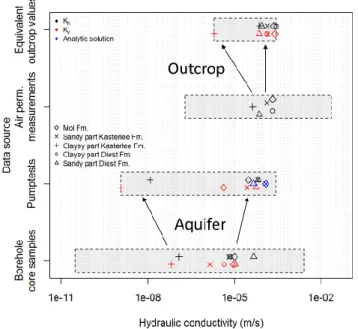
Fig. 6. Comparison of geometric mean K values obtained from

borehole core samples, pump tests, outcrop air-permeameter mea-surements and calculated equivalent values. The gray boxes repre-sent the data limits, and the arrows indicate the contrasting effects of upscaling for the aquifer and aquitard units.

A comparison between the outcrop data (air-permeameter-based geometric meanK values and the calculated corre-sponding equivalent values) and the subsurface data (bore-hole core geometric mean K values and the pump test val-ues) is shown in Fig. 6. It reveals the overall range is small-est for the outcrop data, both at the smallsmall-est measurement scale (data for air-permeameter measurements spans 5 or-ders of magnitude versus 8 oror-ders of magnitude for borehole cores) and at the largest scale (calculated equivalent outcrop

K values show a range of ∼ 2 orders of magnitude versus

∼5 orders of magnitude for pump tests). It is further evi-dent that the outcrop-based equivalent K values are system-atically higher than the mean borehole core values; a better correspondence is achieved with the pump test values.

Because a pump test represents a large support volume, easily tens to hundreds of m3, small-scale heterogeneities have much less effect on such large-scale Kvalues, hence the smaller data range. Furthermore, the support volume is commensurate with the computational domains used to cal-culate equivalent outcrop values. Overall the pump test val-ues are generally only slightly smaller than the equivalent outcrop values, except for the clayey part of the Kasterlee Fm. for which the discrepancy is about three to four orders of magnitude. This again emphasizes the need for a correction if outcrop K values are used to inform building conceptual groundwater models. Correction models such as those from Fig. 4 would account for impacts of different compaction

Fig. 7. Comparison of the vertical anisotropy factors derived from

the geometric mean K values from Fig. 6. The pluses between round and square brackets represent respectively the parameter value ob-tained by Gedeon and Mallants (2012) using regional inverse mod-elling and the value representing a part of the aquitard in the original Dessel 2 pump test interpretation by Lebbe (2002).

and/or weathering processes, especially for the more clay-bearing sediments.

The arrows in Fig. 6 indicate different effects of upscaling for the aquifer and aquitard units. Moving from the sample (cm scale) to the pumptest scale (metre scale) in most cases increases the aquifer geometric mean K values by one order of magnitude, while the outcrop values remain more or less constant when geometric means are compared with effective values. Unlike the other formations, upscaling the clayey part of the Kasterlee Fm. data results in a decrease of the aver-age K values, for both Kvand Khpertaining to the aquifer

and for outcrop Kv. This indicates that in both the outcrop

and aquifer sediments of this particular lithostratigraphic unit a significant amount of small-scale heterogeneity is present (i.e. clay lenses) which significantly decreases the magnitude of the calculated effective K values.

Faulting could be another process involved enhancing dis-crepancies between small and large measurement supports. However, this process is considered to be absent as the study area is known as a zone of low seismic and limited tectonic activity (De Craen et al., 2012).

A comparison of the vertical anisotropy values (Kh/Kv)

is shown in Fig. 7. The Kh/Kv ratios based on the

geo-metric means of the 100 cm3borehole cores lies between 1 and 5. The two lithostratigraphical units with the highest

Kh/Kvvalues are the sandy parts of the Kasterlee and

Di-est Fm., which are influenced by some outliers that probably belong to the under- or overlying units. The equivalent out-crop Kh/Kvvalues are less than the corresponding borehole

core anisotropy values, except for the clayey parts of the Di-est and Kasterlee Fm. For the latter Kh/Kvincreased more

(9)

Table 2. Overview of fitted spherical variogram model

parame-ters for the vertical experimental variograms (range = correlation length). The outcrop data is taken from Rogiers et al. (2013a). The root mean squared error (RMSE) is provided as a measure of good-ness of fit.

Sediment Parameter Outcrop Borehole Both

Mol formation Nugget 0.05 0.13 0.04 Sill – 0.41 0.41 Range (m) – 19.66 12.46 Type Spherical RMSE 0.005 0.046 0.036

Kasterlee formation: sandy part

Nugget 0.16 0 0.25

Sill 0.35 0.13 –

Range (m) 1.36 2.9 –

Type Spherical

RMSE 0.069 0.014 0.145

Kasterlee formation: clayey part

Nugget 0.4 2.07 0.6

Sill 0.2 – 1.32

Range (m) 0.36 – 2.2

Type Spherical

RMSE 0.127 0.303 0.653

Diest formation: clayey part

Nugget 0.35 0.23∗ 0.33

Sill 0.2 0.24 0.14

Range (m) 2.07 1.17 1.12

Type Spherical

RMSE 0.044 0.097 0.076

Diest formation: sandy part

Nugget 0.02 0.07 0.1 Sill 0.18 0.11 0.06 Range (m) 0.6 13.34∗ 13.34∗

Type Spherical

RMSE 0.015 0.019 0.044 ∗_{Fixed during variogram model fit.}

than one order of magnitude, when moving from the borehole core to the outcrop scale. The pump test anisotropy values mostly show larger values compared to those from the bore-hole cores, with a maximum vertical anisotropy of 10. The original Dessel 2 pump test interpretation by Lebbe (2002) yielded K values for the clayey part of the Kasterlee Fm. and mentions a vertical anisotropy factor of 190 for part of the aquitard. This value was obtained by inverse modelling of the pump test, but due to a limited drawdown across the aquitard, the optimized parameter values remain highly un-certain. A more reliable estimate is probably obtained from the more regional modelling of the Neogene aquifer and the flow across the aquitard by Gedeon and Mallants (2012). They obtain a vertical anisotropy of 148 by inverse condition-ing on regional piezometric observations above and below the aquitard. The high vertical anisotropy determined from the outcrop supports these values, and indicates that such large values might be more realistic at larger scales.

3.6 Spatial variability

The vertical spatial variability for the outcrop and borehole data (Khonly) is compared in Fig. 8 and Table 2. For the Mol

Fig. 8. Comparison between vertical experimental and modelled

semivariograms (fitted using a least squares approach) for out-crop and borehole data. (A) Mol Fm., (B) sandy Kasterlee Fm.,

(C) clayey Kasterlee Fm., (D) clayey Diest Fm., and (E) sandy

Di-est Fm. The fit diagnostics are provided in Table 2.

Fm., the outcrop data overall shows less variability (smaller semi-variance) than the borehole core samples; but corre-spond well with the experimental borehole variogram at the centimetre to metre scale. The larger total sill for borehole (0.13 + 0.41) compared to outcrop (0.05) is a reflection of the larger variability captured by the borehole data. This larger variability is caused in part by combining two local stratigraphical subunits into the Mol Fm. (see Beerten et al., 2010) with thin gravel layers and clay lenses at their inter-face. The borehole data also displays a larger vertical spatial range (i.e. 20 m) than the outcrop (i.e. pure nugget), owing to samples being collected from a much larger vertical sam-pling window (up to 20 m) and multiple boreholes spread

(10)

tured by the outcrop samples may be used as surrogate for the variability in boreholes. Despite the presence of spatial correlation in the both data sets, the joint model fit shows a pure nugget because of the high semivariance values for the outcrop data.

The clayey Kasterlee Fm. shows the largest spatial vari-ability of all lithological units for both the outcrop and bore-hole data. While the outcrop shows some spatial correlation, the borehole model shows a pure nugget. The borehole cores show higher variability due to the clay-rich lenses and corre-spondingly low K values, which are altered in the outcrops, but only the first data point at 0.5 m is contradicting the out-crop data. The joint model fit does reveal their compatibility, and shows spatial correlation up to a few metres. This model might be more useful than the individual variogram models due to the integration of different scales.

Most of the clayey Diest Fm. outcrop data seems to be compatible with the borehole core spatial variability. All three model fits show a range of one to two metres, and sim-ilar total sills. The sandy Diest Fm. also exhibits simsim-ilar to-tal sill in all three cases, with a larger spatial range for the borehole data. The joint model fit is compatible with that of the borehole data, but shows a higher nugget due to the higher semivariances in the outcrop data. The sill and range for the variograms that have not reached a constant semi-variance within a lag distance of 14 m (Fig. 8a and e), are highly uncertain as a linear model would provide an equally poor description of the data as the used spherical model. The semivariance within the distance range of the experimental data (up to 10–15 m) is, however, hardly affected by this.

Overall, the borehole data exhibit larger correlation lengths than the outcrop data. The total sills are mostly sim-ilar, except for two cases were the borehole data clearly en-compasses more heterogeneity. Three out of five experimen-tal variograms are overlapping at certain locations, indicat-ing that at certain scales both data sets exhibit similar spatial variability. Fitting of the joint data sets results in these cases in more robust variogram models. For the Mol formation, the variogram model root mean squared errors (RMSE; Table 2) show that fitting both data sets simultaneously improves the fit, mainly due to the very low outcrop semivariances that are compatible with the borehole data. For the sandy part of the Kasterlee formation, the data sets are not compatible and the joint pure nugget fit shows the highest RMSE. For the clayey Kasterlee formation, both data sets seem to be compatible,

tive and quantitative insight about such properties for similar aquifer and aquitard sediments.

4 Perspectives

Despite the limitations of and systematic differences between the outcrop and borehole data sets, we have demonstrated that outcrop studies can provide useful information for devel-oping more reliable groundwater flow and contaminant trans-port models. Because of the systematic differences observed here between outcrop and subsurface sediments, the obtained outcrop K values are not directly applicable in groundwa-ter flow modelling, unless a correction is applied. Further-more, the different K distributions are comparable at least in a relative way, and linear scaling based on deciles was shown to be relatively accurate. In other words, results such as the spatial heterogeneity models, the equivalent vertical anisotropy factors, and relative differences between the dif-ferent sediments provide us with information useful to guide conceptual groundwater flow model building and constrain-ing model parameterization.

Potential applications of our findings for building con-ceptual and numerical models of groundwater flow include (i) where possible highly structured heterogeneity should ei-ther be represented explicitly in the models or use should be made of appropriate geostatistical tools (e.g. multiple point statistics) based on detailed structural information visible in and quantifiable from outcrops; (ii) use of the obtained equivalent vertical anisotropy factors can influence concep-tual model choices for isotropy/anisotropy for certain units, and the actual value represents a minimum of the parame-ter range in larger scale groundwaparame-ter flow simulations (es-pecially in a layered stratigraphical setting); (iii) to avoid over-parameterization, ratios between K values of different units can be fixed during model optimization (e.g. Gedeon and Mallants, 2012) using the ratios obtained from equiva-lent outcrop estimates; and (iv) use of the obtained outcrop variogram models can complement information from a larger scale (e.g. boreholes), or be used for small-scale geostatisti-cal simulations for detailed logeostatisti-cal transport simulations. All these applications will be most beneficial when combined with the traditional borehole coring and measurements and other invasive and non-invasive subsurface characterization techniques.

(11)

5 Conclusions

Analysis of outcrop sediments considered to be analogues for various lithostratigraphical units within a sedimentary aquifer provided a qualitative understanding of aquifer and aquitard stratigraphy and a quantitative estimate about K variability at the centimetre–metre scale. Comparison be-tween outcrop and independent borehole core K values re-vealed significant differences between both data sets. Such differences are believed to be induced mainly by weather-ing, different palaeoenvironmental conditions and differen-tial compaction, and can be corrected for as was demon-strated on the basis of a linear model. Hence, outcrop infor-mation can be used for building better stratigraphic models including determination of spatial structure by variogram fit-ting for further use in geostatistical simulations. Moreover, the relative variability in K values with similar coefficients of variation for borehole and outcrop K, and the derived anisotropy values are very useful to get a more complete un-derstanding of the heterogeneity within the Neogene aquifer. Comparison of outcrop and borehole K values demon-strated the borehole K probability density functions had broader peaks, longer tails towards low values, and the pres-ence of a systematic bias. The reasons behind this discrep-ancy are manifold, and include weathering of the outcrop sediments and a lesser degree of consolidation and associated stress states in outcrops. Also, measurements performed on outcrops sometimes several tens of kilometres away from the main study site may further invoke differences in K. Grain-size analyses showed that the sediments from the investigated outcrops and boreholes are similar but not necessarily ex-actly the same. Clay migration and bioturbation in the out-crop sediments probably contributed to the observed discrep-ancies, as well as slight differences in palaeoenvironmental settings. The degree of (over)consolidation and stress states might also have an impact, but further research is needed to confirm or quantify this, as trends with the current depth of the sediments are hard to detect due to the alternation of dif-ferent lithologies.

Based on all data a linear scaling relationship was derived (r2= 0.7) that permits rescaling of outcrop K values to their subsurface equivalents. For most individual units, the differ-ences between outcrop and subsurface sediments were simi-lar (except for the extremes of the distributions). The sandy part of the Diest Fm. however showed a considerably better fit between outcrop and aquifer than the other cases.

In a comparison with K values obtained through other means, outcrop-based equivalent K values were systemati-cally higher than those from pump tests (especially for the clayey part of the Kasterlee Fm.), whose support volumes are considerably larger than the simulation domains consid-ered in the outcrops. Mean borehole core samples resulted in the overall smallest K values. Smaller compaction at shallow depth and long-term biophysical weathering processes pre-sumably contributed to outcrop equivalent K values being

larger than any other estimate of large-scale K available in this study.

In most cases the semivariograms for the outcrop and borehole data are compatible. Only for the sandy Kasterlee Fm. the outcrop data clearly shows higher variability than the borehole data. Spatial correlation (i.e. increasing semivari-ance with distsemivari-ance) is present in most cases, either in the out-crop or borehole data, or both. The clayey Diest Fm. shows however a pure nugget effect for both data sets. For the Mol Fm. and the clayey Kasterlee Fm. both data sets complement each other resulting in more robust semivariogram model fits. For the sandy Diest Fm. there seems to be a discrepancy in the range between both data sets.

Given the small number and limited size of the studied outcrops, transfer of information from outcrops to the cor-responding aquifer sediments can be improved by expand-ing the number of outcrops for the same lithostratigraphi-cal units. In addition, more complementary aquifer informa-tion could be collected for developing a depth dependency in aquifer K that incorporates effects of compaction which could then be used to rescale outcrop K values to sediment values at a given depth. Such information, together with geo-statistical parameters, may be used as input or prior informa-tion to stochastic flow models.

Next to the quantitative information tested in this paper, information about facies geometry, like the alternating clay and sand layers within the clayey Kasterlee Fm., cannot be revealed easily using available in situ methods, and repre-sents very important qualitative knowledge obtained from outcrops.

Acknowledgements. The authors wish to acknowledge the Fund

for Scientific Research – Flanders for providing a Postdoctoral Fellowship to Marijke Huysmans. ONDRAF/NIRAS, the Belgian Agency for Radioactive Waste and Enriched Fissile Materials, is acknowledged for providing the borehole data. Findings and conclusions in this paper are those of the authors and do not necessarily represent the official position of ONDRAF/NIRAS. Edited by: P. Grathwohl

References

Bakke, S. and Øren, P.: 3-D pore-scale modelling of sandstones and flow simulations in the pore networks, Soc. Petrol. Eng. J., 2, 136–149, 1997.

Bayer, P., Huggenberger, P., Renard, P., and Comunian, A.: Three-dimensional high resolution fluvio-glacial aquifer analog: Part1: Field study, J. Hydrol., 405, 1–9, 2011.

Beerten, K., Wemaere, I., Gedeon, M., Labat, S., Rogiers, B., Mal-lants, D., Salah, S., and Leterme, B.: Geological, hydrogeolog-ical and hydrologhydrogeolog-ical data for the Dessel disposal site. Project near surface disposal of category A waste at Dessel, Version 1, NIRAS/ONDRAF, Brussels, Belgium, p. 273, 2010.

(12)

Case 1 (SFC1), External Report of the Belgian Nuclear Research Centre, Mol, Belgium, p. 120, 2012.

Flint, S. S. and Bryant, I. D. (Eds.): The Geological Modelling of Hydrocarbon Reservoirs and Outcrop Analogues, Blackwell Publishing Ltd., Oxford, UK, 1993.

Fobe, B.:. Litologie en litostratigrafie van de Formatie van Kasterlee (Plioceen van de Kempen), Natuurwetenschappelijk tijdschrift, 75, 35–45, 1995

Gedeon, M. and Mallants, D.: Sensitivity analysis of a com-bined groundwater flow and transport model using local-grid refinement: A case study, Math. Geosci., 44, 881–899, doi:10.1007/s11004-012-9416-3, 2012.

Gulinck, M.: Essai d’une carte géologique de la Campine, Etat de nos connaissances sur la nature des terrains néogènes recoupés par sondages, Symposium Stratigraphie Néogène Nordique (Gand 1961), Mém. Soc. Belge Géol., 6, 30–39, 1963.

Iversen, B. V., Moldrup, P., Schjonning, P., and Jacobsen, O. H.: Field Application of a Portable Air Permeameter to Characterize Spatial Variability in Air and Water Permeability, Vadose Zone J., 2, 618–626, 2003.

Klute, A.: Laboratory measurements of hydraulic conductivity of saturated soil, in: Methods of soil analysis, Part 1, edited by: Black, C. A., Agronomy, 9, 210–220, 1965.

Laga, P.: The Neogene deposits of Belgium, Guide book for the field meeting of the Geologists’ Association London, Belgian Geolog-ical Survey, Brussel, 1–31, 1973.

Lambert, M. R., Cole, R. D., and Mozley, P. S.: Controls on per-meability heterogeneity in the Tocito Sandstone (Upper Creta-ceous), northwest New Mexico, in: Mesozoic geology and pale-ontology of the Four Corners Region, edited by: Anderson, O. J., Kues, B. S. and Lucas, S. G., Guidebook, 48th Field Conference, New Mexico Geological Society, New Mexico, 217–228, 1997. Lebbe, L.: Interpretatie van een pompproef uitgevoerd te

Mol, Rapport GROMO2002/07-RUG, Vakgroep Geologie en Bodemkunde, University Gent, September 2002.

Li, L., Zhou, H., and Gómez-Hernández, J. J.: A Comparative Study of Three-Dimensional Hydraulic Conductivity Upscaling at the MAcro-Dispersion Experiment (MADE) site, Columbus Air Force Base, Mississippi (USA), J. Hydrol., 404, 278–293, 2011.

Mallants, D., Mohanty, B. P., Vervoort, A., and Feyen, J.: Spatial analysis of saturated hydraulic conductivity of a macroporous soil, Soil Technol., 10, 115–131, 1997.

Mažvila, J., Vaicys, M., and Beniušis, R.: Causes and consequences of the vertical migration of fine soil fractions, Žemes Ukio Mok-slai, 15, 36–41, 2008.

14 June 2011.

Øren, P., Bakke, S., and Arntzen, O.: Extending predictive capabil-ities to network models, SPE Annual Technical Conference and Exhibition, San Antonio, Texas, 324–336, 1998.

Pebesma, E. J.: Multivariable geostatistics in S: the gstat package, Comput. Geosci., 30, 683-691, 2004.

Pettersen, O.: Sandstone compaction, grain packing and Criti-cal State Theory, Petrol. Geosci., 13, 63–67, doi:10.1144/1354-079305-677, 2007.

Pringle, J. K., Westerman, A. R., Clark, J. D., Drinkwater, N. J., and Gardiner, A. R.: 3D high-resolution digital models of outcrop analogue study sites to constrain reservoir model uncertainty: an example from Alport Castles, Derbyshire, UK, Petrol. Geosci., 10, 343–352, 2004.

Pringle, J. K., Howell, J. A., Hodgetts, D., Westerman, A. R., and Hodgson, D. M.: Virtual outcrop models of petroleum reservoir analogues: a review of the current state-of-the-art, First break 24, European Association of Geoscientists and Engineers (EAGE), Houten, 33–42, 2006.

Rogiers, B., Mallants, D., Batelaan, O., Gedeon, M., Huysmans, M., and Dassargues, A.: Estimation of hydraulic conductivity and its uncertainty from grain-size data using GLUE and artificial neural networks, Math. Geosci., 44, 739–763, doi:10.1007/s11004-012-9409-2, 2012.

Rogiers, B., Beerten, K., Smeekens, T., Mallants, D., Gedeon, M., Huysmans, M., Batelaan, O., and Dassargues, A.: The usefulness of outcrop analogue air permeameter measurements for analysing aquifer heterogeneity: Quantifying spatial vari-ability in outcrop hydraulic conductivity, Hydrol. Process., doi:10.1002/hyp.10007, in press, 2013a.

Rogiers, B., Beerten, K., Smeekens, T., Mallants, D., Gedeon, M., Huysmans, M., Batelaan, O., and Dassargues, A.: Derivation of flow and transport parameters from outcropping sediments of the Neogene aquifer, Belgium, Geologica Belgica, 16, 129–148, 2013b.

Teutsch, G., Klingbeil, R., and Kleineidam, S.: Numerical mod-elling of reactive transport using aquifer analogue data, in: Groundwater Quality: Remediation and Protection (Proceedings of the GQ’98 Conference held at Tübingen, Germany, September 1998), IAHS Publ., 250, 375–379, 1998.

van Ranst, E. and De Coninck, F.: Evolution of glauconite in imper-fectly drained sandy soils of the Belgian Campine, Z. Pflanzen-ern. Bodenk., 146, 415–426, 1983.