Anchors of morphological operators and algebraic openings

(1)

M. VANDROOGENBROECK. Anchors of morphological operators and algebraic openings. Advances in Imaging and Electronic Physics, volume

158, chapter 5, pages 173–201, 2009.

doi :10.1016/S1076-5670(09)00010-X

Anchors of Morphological Operators and Algebraic Openings

M. V

AN

D

ROOGENBROECK

University of Liège, Department of Electrical Engineering and Computer Sciences Montefiore B28, Sart Tilman, B-4000 Liège, Belgium

ABSTRACT

Opening and closing operators play an important role in the field of mathematical morphology, mainly because of their useful property of idempotence, which is similar to the notion of ideal filter in linear filtering. From a theoretical point of view, the study of openings has focused on the algebraic characterization of the operators themselves. Morphological filters have been studied for more than 30 years; the effects of the first filters (erosions, openings, and so on) are known in depth. In discussing the effects of a filter, it is not only the operator that is studied but also its relationship with the processed function or image and, in the particular case of mathe-matical morphology, the structuring element. In addition, there are several approaches to this analysis. For example, the analysis can consider the whole function or some subparts of the function, as in Van Droogenbroeck and Buckley (2005), who introduced the notion of

morpho-logical anchors. Anchors were defined in the context of morphomorpho-logical openings, as defined

by the cascade of an erosion followed by a dilation. The extension to other kinds of openings is not straightforward. Despite the fact that all morphological openings induce the appearance of anchors, some opening operators (like the quantization opening defined in this chapter) might have no anchors. This chapter presents the theory of anchors related to morphological erosions and openings, and establishes some properties for the extended scope of algebraic openings. It is shown under which circumstances anchors exist for algebraic openings and how to locate some anchors; for example, it suffices for an opening to be spatial or shift-invariant to guar-antee the existence of anchors. As for morphological openings, the existence of anchors may help clarify some algorithms or lead to new algorithms to compute algebraic openings.

Chapter outline

1. Introduction

1.1 Terminology and Scope

1.1.1 The Notion of Idempotence 1.2 Towards Openings

1.3 Anchors

2. Morphological Anchors 2.1 Set and Function Operators 2.2 Theory of Morphological Anchors 2.3 Local Existence of Anchors

2.4 Algorithmic Properties of Morphological Anchors 3. Anchors of Algebraic Openings

3.1 Spatial and Shift-Invariant Openings 3.2 Granulometries

4. Conclusions References

(2)

1. INTRODUCTION

Over the years mathematical morphology, a theory initiated by Matheron (1975) and Serra (1982), has grown to a major theory in the field of nonlinear image processing. Tools of math-ematical morphology, such as morphological filters, the watershed transform, and connectivity operators, are now widely available in commercial image processing software packages and the theory itself has considerably expanded over the past decade (Najman and Talbot, 2008). This expansion includes new operators, algorithms, methodologies, and concepts that have led math-ematical morphology to become part of the mainstream of image analysis and image-processing technologies.

The growth in popularity is due not only to the theoretical work of some pioneers but also to the development of powerful tools for image processing such as granulometries (Matheron, 1975), pattern spectrum analysis-based techniques (Maragos, 1989) that provide insights into shapes, and transforms like the watershed (Beucher and Lantuéjoul, 1979; Vincent and Soille, 1991) or connected operators (Salembier and Serra, 1995) that help to segment an image. All these operators have been studied intensively and tractable algorithms have been found to implement them effectively, that is, in real time on an ordinary desktop computer.

Historically, mathematical morphology is considered a theory that is concerned with the pro-cessing of images, using operators based on topological and geometrical properties. According to Heijmans (1994), the first books on mathematical morphology discuss a number of mappings on subsets of the Euclidean plane, which have in common that they are based on set-theoretical operations (union, intersection, complementation), as well as translations. More recently re-searchers have extended morphological operators to arbitrary complete lattices, a step that has paved the way to more general algebraic frameworks.

The geometrical interpretation of mathematical morphology relates to the use of a probe which is a set called structuring element. The basic idea in binary morphology is to probe an image with the shape of the structuring element and draw conclusions on how this shape fits or misses the regions of that image. Consequently, there are as many interpretations of an image as structuring elements, although one often falls back to a few subset of structuring elements, such as lines, squares, balls, or hexagons. In geometrically motivated approaches to mathematical morphology, the focus clearly lies on the shape and size of the structuring element.

Algebraic approaches do not refer to geometrical or topological concepts. They concentrate on the properties of operators. Consequently, algebraic approaches embrace larger classes of operators and functions. But in both approaches the goal is to characterize operators to help design solutions useful for image processing applications.

1.1. Terminology and Scope

LetR and Z be the set of all real and integer numbers, respectively. In this chapter, we consider transformations and functions defined on a space E , which is the continuous Euclidean space_Rn or the discrete space _Zn, where n≥ 1 is an integer. Elements of E are written p, x, . . ., while subsets of elements are denoted by upper-case letters X , Y, . . . Subsets of _R2 are also called

(3)

158, chapter 5, pages 173–201, 2009.

doi :10.1016/S1076-5670(09)00010-X

3 binary sets or images because two colors suffice to draw them (elements of X are usually drawn

in black, and elements that do not belong to X in white).

Next we introduce an order on P(E ), the power set comprising all subsets of E , that results from the usual inclusion notion. X is smaller or equal to Y if and only if X ⊆ Y . Note that we decide to encompass the case of equality in contrary to strict inclusion⊂. The power set P(E ) with the inclusion ordering is a complete lattice (Heijmans, 1994).

This chapter also deals with images. Images are modeled as functions (denoted as f , g, . . .), that map a non-empty set E of E into R, where R is a set of binary values {0, 1}, a discrete set of grey-scale values{0, . . . , 255}, or a closed interval [0, 255], defining, respectively, binary, grey-scale or continuous images. The ordering relation ≤ is given by “ f ≤ g if and only if f(x) ≤ g(x) for every x ∈ E.” It can be shown that the space Fun(E , R) of all functions and ≤ form a complete lattice, which means among others that every subset of the lattice has an infimum and a supremum.

The frameworks of P(E ) and ⊆, or Fun(E , R) and ≤, are equivalent as long as we deal with complete lattices. Most results can thus be transposed from one framework to the other. In the following we arbitrary decide to restrict functions to be single-valued grey-scale images. Also, for convenience, we use the unique term operators to refer to operations that map sets of E into E or handle Fun(E , R). In addition, we restrict the scope of this chapter to operators that map sets to sets, or functions to functions. This implies that both the input and the output lattices are the same, or equivalently, that there is only one complete lattice under consideration. Operators are denoted by greek lettersε,δ,γ,ψ, . . .

1.1.1. The Notion of Idempotence

Linear filters and operators are common in many engineering fields that process signals. As an analogy, remember that every computer with a sound card contains a hardware module that prefilters the acquired signal before sampling to prevent aliasing. Likewise, digital signals are converted to analog signals by means of a low-pass filter.

The concept of a reference filter called an ideal filter is often used to characterize linear filters. Ideal filters have a binary transmittance with only two values: 0 or 1. Either they retain a fre-quency or they drop it. Ideal filters stabilize the result after a single pass; further applications do not modify the result any more in the spectral domain (nor in the spatial domain!). Unfortunately, it can be shown that because practical linear filters have a finite kernel in the spatial domain, they cannot be ideal. It might be impossible to build ideal filters, but they nevertheless serve as a reference because it is pointless to repeat the filtering process.

The notion of frequency is irrelevant in nonlinear image processing. Nonlinear operators op-erate in the initial domain, either globally or locally. An important class of nonlinear operators computes rank statistics inside a moving window. For example, the median operator that selects the median from a collection of values taken inside a moving local window centered on x and that allocates the median value toψ( f )(x) is known to be efficient for the removal of salt-and-pepper noise (Figure1). However, in some cases, the median filter oscillates as shown in Figure2.

(4)

(a) (b) (c)

FIGURE 1. Effect of a median filter. (a) Original grey-scale image, (b) original image corrupted by noise, and (c) filtered image.

... ... ... ... ... ...

FIGURE2. Successive applications of a three-pixel wide median filter on a binary image may result in oscillations.

Oscillations may not be common in practice, but they still cast doubts on the significance of the output function. Therefore, the behavior of median operators has been characterized in terms of root signals. Technically, a root signal f of an operator, which is sometimes called a fixed

point, is a function that is invariant to the applications of that operator for each location:∀x ∈ E ,

ψ( f )(x) = f (x), where f is the root signal.

The existence of root signals is not restricted to the median operator. Let us consider a simple example of a one-dimensional constant function g(x) = k and a linear filter with an impulse response h(x). The filtered signal r(x) is the convolution of g(x) by h(x): r(x) =R+∞

−∞ g(t − x)h(t)dt = kR+∞

−∞h(t)dt = kH (0), where H (0) is the Fourier transform of h(t) taken for f = 0.

In the case of an ideal filter, H (0) = 1 so that r(x) = k = g(x). This illustrates that, up to a constant, root signals for linear operators typically include constant-valued or straight-line signals.

For nonlinear operators, there is a property somewhat similar to that of an ideal filter for linear processing. Mathematical morphology uses a property called idempotence.

(5)

158, chapter 5, pages 173–201, 2009.

doi :10.1016/S1076-5670(09)00010-X

5

Definition 1. Consider an operator ψ on a complete lattice (L , ≤), and let X be an arbitrary element of L . An operatorψ is idempotent if and only if

(1) ψ(ψ(X)) =ψ(X)

for any X of L . In the following, we use this notation or the operator composition: ψψ =ψ. In contrast to the case of ideal filters, it is possible to implement idempotent operators. There-fore, the property is part of the design of filters and not just a goal; idempotence is chosen as one of the compulsory property for the operator. This explains why many idempotent operators have been proposed: algebraic filters, morphological openings, attribute openings,...

Idempotence might be one of the requirements in the design of an operator, it does not suffice! For example, an operatorψ that maps every function to g(x) = −∞is idempotent but useless. Hereafter, we present additional properties to complete the algebraic framework and elaborate on the formal definition of openings.

1.2. Toward Openings

By definition, a notion of order exists on a complete (L , ≤). The property of increasingness guarantees that an order between objects in the lattice is preserved (remember that we deal only with objects that belong to a unique lattice, that is X ,ψ(X) ∈ L and there is only one notion of order≤). That is,

Definition 2. The lattice operatorψ is called increasing if X≤ Y impliesψ(X) ≤ψ(Y ) for every X , Y ∈ L .

Letψ be an operator on L , and let X be an element of L for which ψ(X) = X. Then X is called invariant under ψ or, alternatively, a fixed point of ψ. The set of all elements invariant underψ is denoted by Inv(ψ) and is called the invariance domain ofψ. The Tarski’s fixpoint theorem specifies that the invariance domain Inv(ψ) of an increasing operatorψ on a complete lattice is nonempty.

Increasingness builds a bridge between ordering relations before and after the operator. But, as X andψ(X) are defined on the same lattice, one can also compare X toψ(X), leading us to define additional properties:

Definition 3. Let X , Y be two sets (or functions) of a lattice (L , ≤). An operatorψ on L is called

• extensive ifψ(X) ≥ X for every X ∈ L ; • anti-extensive ifψ(X) ≤ X for every X ∈ L .

In more practical terms, increasingness tells us if an order in the source lattice is preserved in the destination lattice, idempotence if the application of the operator stabilizes the results, and extensivity if the result is smaller or larger than its source. Figure 3 shows these remarks in illustrative terms: f(x) ≤ g(x) impliesγ( f ) ≤γ(g),γ( f (x)) ≤ f (x), andγ(g(x)) ≤ g(x).

(6)

(a) f(x) (b)γ( f (x))

(c) g(x) (d)γ(g(x))

FIGURE 3. Illustrations of increasingness and anti-extensivity. (a) and (b) Orig-inal grey-scale image f(x) and after processing with an opening operator γ; (c) and (d) Similar displays for a whiter image g(x).

When an operatorψ is both increasing and idempotent, it is called an algebraic filter. Regard-ing the extensivity property, there are two types of algebraic filters: anti-extensive or extensive algebraic filters are respectively called algebraic openings or algebraic closings. Openings and closings share the common properties of increasingness and idempotence, but are dual with re-spect to extensivity. Thanks to this duality, we can limit the scope of this chapter to openings; handling closings brings similar results.

Figure4shows the effect of an algebraic opening Qnthat rounds grey-scale values to a closest inferior multiple of an integer n; this operator is called quantization in signal processing. It is

(7)

158, chapter 5, pages 173–201, 2009.

doi :10.1016/S1076-5670(09)00010-X

7

(a) f(x) (b) Q10( f (x)) (c) Q50( f (x))

FIGURE 4. Quantization operator. (a) Original grey-scale image, (b) image rounded to the closest inferior multiple of 10, and (c) image rounded to the closest inferior multiple of 50.

increasing, anti-extensive, and idempotent, but it should be noted that if none f(x) is a multiple of n, then f(x) 6=ψ( f (x)) for all x ∈ E . In other words, quantization may produce values that are not present in the original image and thus have questionable statistical significance.

Note that the definition of order is a pointwise property. f(x) is compared with g(x) orγ( f x)) but not compared with the value at a different location (called pixel in image analysis). In prac-tice, however, neighboring pixels share some common physical significance that, for example,

rank operators explore. A rank operator of rank k within a discrete sliding window centered at

a given location x is obtained by sorting in ascending order the values falling inside the window and by selecting as output value for x the kth value in the sorted list. Some of the best-known rank operators are the local minimum and maximum operators. In mathematical morphology, these operators are referred to as erosion and dilation, respectively, and the window itself is termed a

structuring element or a structuring set. There filters are also referred to as min- or max-filters in

the literature. The presence of some interaction between neighboring pixels introduced by rank operators is why their characterization becomes more challenging.

Consider a complete lattice(L , ≤). To elaborate on the notion of neighborhood, we propose the definition of a property called spatiality.

Definition 4. An operatorψ on(L , ≤) is said to be spatial if for every location x ∈ E and for every function f , there exists y∈ E such that

(2) ψ( f (x)) = f (y),

(8)

As explained previously, the quantization operator is not spatial because it does not consider the neighborhood of x.

Assuming that an image is the result of an observation, the smaller the choice of the neigh-borhood for finding y, the higher the physical correlation between pixels will be. On purpose, there is no notion of distance between x and y in the definition of spatiality, although one hopes that operators with a reasonable physical significance should restrict the search for y to a close neighborhood of x.

Spatiality constrains operators to select values in the neighborhood of a pixel. But the under-lying question that is twofold remains: (1) Does an operator drive any input to a root signal (this is called the convergence property), and (2) if not, do oscillations propagate? Root signals have been studied with a particular emphasis on median filters (Arce and Gallagher, 1982; Arce and McLoughlin, 1987; Astola et al., 1987; Eberly et al., 1991; Eckhardt, 2003; Gallagher and Wise, 1981).

The convergence property is of no particular interest for idempotent operators, asψ(ψ( f )) =

ψ( f ), so that the question becomes that of determining the subset of locations x ∈ E such that f(x) =ψ( f (x)). In different terms, the study of the invariance domain Inv (ψ) is a key to a better understanding ofψ; indeed, characterizing locations for a function f with respect toψ can help implement the operator (as shown in Van Droogenbroeck and Buckley, 2005).

1.3. Anchors

To analyze the behavior of some operators, we introduce the concept of anchors. We now define this concept, which can be seen as an extension of that of roots. An anchor is essentially a version of the root notion where the domain of definition is reduced to a subset of it.

Definition 5. Given a signal f and an operator ψ on a complete lattice (L , ≤), the pair com-prising a location x in the domain of definition of f and the value f(x) is an anchor for f with respect toψ if

(3) ψ( f )(x) = f (x).

In marketing terms, one would say “The right value at the right place.”

The set of anchors is denoted A_ψ( f ). Note that Definition5differs from the initial definition provided in Van Droogenbroeck and Buckley (2005) to emphasize the role of both the location

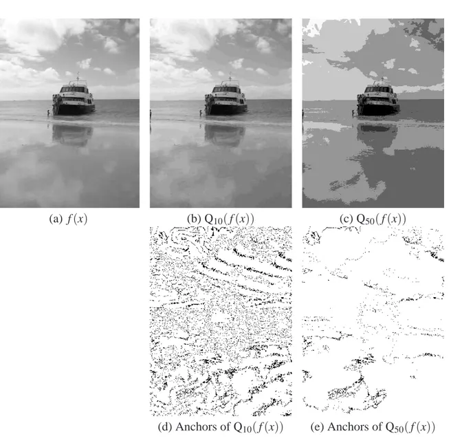
x and the value of f(x). We provide an illustration in Figure 5. In this particular case, there is no evidence that anchors should always exist. Take a grey-scale image whose values f(x) are all odd, then Q2( f ) has no anchor, although f and Q2( f ) look identical.

The existence of anchors is an open issue. Also it is interesting to determine whether an order between operators implies a similar inclusion order between anchor sets. In general, γ1 ≤γ2

is no guarantee to establish an inclusion of their respective anchor sets. However, drawings (d) and (e) of Figure 5 suggest that AQ50( f ) ⊆ AQ10( f ), which is true in this case because, in addition to Q50( f ) ≤ Q10( f ), Q50( f ) “absorbs” Q10( f ); more precisely, it is required that

(9)

158, chapter 5, pages 173–201, 2009.

doi :10.1016/S1076-5670(09)00010-X

9

(a) f(x) (b) Q10( f (x)) (c) Q50( f (x))

(d) Anchors of Q10( f (x)) (e) Anchors of Q50( f (x))

FIGURE 5. Quantization operator and anchors whose locations are drawn in black in (d) and (e). (a) Original image, (b) image rounded to the closest infe-rior multiple of 10, (c) image rounded to the closest infeinfe-rior multiple of 50, (d) and (e), respectively, anchors of (b) and (c).

Figure6shows anchors of two other common operators: morphological erosions and openings (detailed further in Section2).

Papers dealing with roots, convergence, or invariance domains focus either on the operator itself or on the entire signal. Anchors characterize a function locally, but they also help in finding algorithms, or interpreting existing algorithms. Van Droogenbroeck and Buckley (2005) pre-sented algorithms applicable to morphological operators based on linear structuring elements and show how they offer an alternative to implementations like the one of van Herk (1992).

(10)

(a) f (b)εB( f ) (c) Anchors ofεB( f )

(d)γB( f ) (e) Anchors ofγB( f ) FIGURE 6. Illustration of anchors [marked in black in (c) and (e)]. (a) Original image, (b) an image eroded by a 3× 3 square structuring element, (c) anchor locations of εB( f ), (d) an image opened by a 3 × 3 square structuring element, and (e) anchor locations ofγB( f ).

In this chapter, we use an algebraic framework, with an eye on the geometrical notions, to ex-pose the notion of anchors. The remainder of this chapter is organized as follows: Section2 re-calls several definitions and details theoretical results valid for morphological operators; anchors related to morphological operators are called morphological anchors. This section rephrases many results presented in Van Droogenbroeck and Buckley (2005). Section 3 extends the no-tion of anchors to the framework of algebraic operators. In particular, we present the concept of algebraic anchors that applies for algebraic openings and closings. The major contribution is the proof that if some operators might have no anchors (remember the case of the quantization

(11)

158, chapter 5, pages 173–201, 2009.

doi :10.1016/S1076-5670(09)00010-X

11

operator Q2 of an image filled with odd grey-scale values), classes of openings and closings,

others than their morphological “brothers,” have anchors, too. 2. MORPHOLOGICAL ANCHORS

After a brief reminder on basic morphological operators, we emphasize the role of anchors in the context of erosions and openings by discussing their existence and density. It is shown that anchors are intimately related to morphological openings and closings (their duals), and that the existence of anchors is guaranteed for openings. Furthermore, it is possible to derive properties useful for the implementation of erosions and openings. Section 3generalizes a few results in the case of algebraic openings.

2.1. Set and Function Operators

If E is the continuous Euclidean space_Rnor the discrete space_Zn, then the translation of x by b is given by x+ b. To translate a given set X ⊆ E by a vector b ∈ E , it is sufficient to translate all the elements of X by b: Xbis defined by Xb= {x + b| x ∈ X}. Due to the commutativity of +, Xb is equivalent to bX, where bX is the translate of b by all elements of X .

Let us consider two subsets X and B of E . The erosion and dilation of these sets by a set B are respectively defined as (4) X⊖ B = \ b∈B X_−b= {p ∈ E | Bp⊆ X}, (5) X⊕ B = [ b∈B Xb= [ x∈X Bx= {x + b| x ∈ X, b ∈ B}.

For X⊕ B, X and B are interchangeable, but not for the erosion, where it is required that Bpbe contained within X . Note that there are as many erosions as sets B. As B serves to enlighten some geometrical characteristics of X , it is called a structuring element or structuring set. Although the window shape might be arbitrary, it is common practice in applied image analysis to use linear, rectangular, or circular structuring elements. If B contains the origin o,

(6) X⊖ B = \ b∈B X_−b=   \ b∈B\{o} X_−b  ∩ X,

which is included in X . Therefore, if o ∈ B, the erosion and dilation are, respectively, anti-extensive and anti-extensive. In addition, both operators are increasing but not idempotent.

Because erosions and dilations are, respectively, anti-extensive and extensive (when the struc-turing element contains the origin), the cascade of an erosion and a dilation suggests itself. This set, denoted by X◦ B, is called the opening of X by B and is defined by

(12)

B

X

X◦ B X• B

FIGURE 7. Opening and closing with a ball B.

Similarly, the closing of X by B is the dilation of X followed by the erosion, both with the same structuring element. It is denoted by X• B and defined by X • B = (X ⊕ B) ⊖ B. Dilations and erosions are closely related although not inverse operators. A precise relation between them is expressed by the duality principle (Serra, 1982) that states that

(8) X⊖ B = (Xc⊕ ˇB)c or X⊕ B = (Xc⊖ ˇB)c,

where the complement of X , denoted Xc, is defined as Xc= {p ∈ E | p 6∈ X}, and the symmetric or transposed set of B⊆ E is the set ˇB defined as ˇB= {−b| b ∈ B}. Therefore, all statements concerning erosions and openings have an equivalent form for dilations and closings and vice versa.

When B contains the origin, X⊖ B is the union of locations p that satisfy Bp⊆ X. When a dilation is applied to this set, the resulting set sums pB-like contributions, which are equivalent to Bp. So X◦ B is the union of Bpthat fits into X :

(9) X◦ B = {Bp| Bp⊆ X}.

In addition, it can be shown that X◦ B is identical to X ◦ Bp, so that the opening does not depend on the position of the origin when choosing B. The interpretation of X◦ B as the union {Bp| Bp⊆

X} is referred to as the geometrical interpretation of the morphological opening. A similar interpretation yields for the closing. The closing is the complementary set of the union of all the translates Bpcontained in Xc. Figure7illustrates an opening and a closing with a ball.

(13)

158, chapter 5, pages 173–201, 2009.

doi :10.1016/S1076-5670(09)00010-X

13

The geometrical interpretation suffices to prove that if X◦ B is not empty, then there are at least #(B) anchors, where #(B) denotes the cardinality or area of B. The existence of anchors for X⊖ B is less trivial; assume that X is a chessboard and B = {p}, where p is located at the distance of one square of the chessboard. In this case, X⊖ B = Xp and X∩ Xp= /0; AX⊖B(X) is

empty. To the contrary, if o∈ B and X ⊖ B is not empty, then the erosion of X by B has anchors. In the following, we define operators on grey-scale images and then discuss the details of anchors related to erosions and openings.

Previous definitions can be extended to binary and grey-scale images. If f is a function and

b∈ E , then the spatial translate of f by b is defined by fb(x) = f (x − b). The spatial translate is also called horizontal translate. The vertical translate, used later in this chapter, of a function

f by a value v is defined by fv(x) = f (x) + v. The vertical translate shifts the function values in the grey-scale domain.

The erosion of a function f by a structuring element B is denoted byεB( f )(x) and is defined as the infimum of the translations of f by the elements−b, where b ∈ B

(10) εB( f )(x) = ^ b∈B f−b(x) = ^ b∈B f(x + b). Likewise, we define the dilation of f by B,δB( f )(x), as

(11) δB( f )(x) = _ b∈B fb(x) = _ b∈B f(x − b).

Note that we consider so-called flat structuring elements; more general definitions using a non-flat structuring elements exist but they are not considered here.

Just as for sets, the morphological openingγB( f ) and closing φB( f ) are defined as composi-tions of erosion and dilation operators:

(12) γB( f ) =δB(εB( f )),

(13) φB( f ) =εB(δB( f )).

Figure8shows the effects of several morphological operators on an image.

Again, εB( f ) and δB( f ), and γB( f ) and φB( f ) are duals of each other (Serra, 1982), which is interpreted as stating that they process the foreground and the background symmetrically. If, by convention, we choose to represent low values with dark pixels in an image (background) and large values with white pixels (foreground), erosions enlarge dark areas and shrinks the foreground.

From all the previous definitions, it can be seen that erosions, dilations, openings, and closings are spatial operators, as defined previously. They use values taken in the neighborhood.

Heijmans (1984) and other authors have shown that set operators can be extended to function operators and hence the entire apparatus of morphology on sets is applicable in the grey-scale case as well. The underlying idea is to slice a function f into a family of increasing sets obtained

(14)

(a) f(x) (b)εB( f ) (c)δB( f )

(d)γB( f ) (e)φB( f ) FIGURE 8. Original image (a), erosion (b), dilation (c), opening (d), and closing (e), with a 15× 15 square.

by thresholding f . Without further details, consider a complete lattice Fun(E , R). We associate a series of threshold sets to f as defined by (Figure9)

(14) X(t) = {x ∈ E | f (x) ≥ t}.

Note that X(t) is decreasing in t and that these sets obey the continuity condition

(15) X(t) =\

s<t

(15)

M. VANDROOGENBROECK. Anchors of morphological operators and algebraic openings. Advances in Imaging and Electronic Physics, volume 158, chapter 5, pages 173–201, 2009. doi :10.1016/S1076-5670(09)00010-X 15 x f(x) t X(t)

FIGURE 9. The profile of a function f and one of its threshold sets.

In addition, there is a one-to-one correspondence between a function and families of sets X(t). In fact, the function f can be recovered from the series of X(t) by means of f (x) =W

{t| x ∈ X(t)}; this is the threshold superposition principle. One interesting application of the correspondence is the possibility to interpret an opening on f as the union of B that fits in the threshold sets. From an implementation point of view, this leads to alternative definitions for morphological opera-tors. Although morphological openings were defined as the cascade of an erosion followed by a dilation [see Eq. (12)], this does not mean that one must implement an opening according to its definition. Examples of the conclusion are, among others, the two implementations of an opening with a line proposed in Van Droogenbroeck (1994) and Vincent (1994). These implementations scans the image line by line and use threshold sets to compute the opening.

2.2. Theory of Morphological Anchors

Let us first consider the simple case of the set opening of X by B. If X is empty, X◦ B is empty, and there is no anchor. Similarly, if X= E and B is finite, X ◦ B = E , all points are again anchors. Leaving these trivial cases, let us take X containing some elements of E . As X◦ B ⊆ X, if X ◦ B is not empty, all locations of X◦ B are anchors. Therefore, in the binary case, anchors do always exist for non-empty sets.

For openings, the notion of anchors is linked to that of invariance domain. Remember that the opening of X by B is the union of the translate of B that fit into X . Therefore, the corresponding invariance domain of X◦ B is given by Inv (X ◦ B) = {Y ⊕ B|Y ∈ P(E )}. Accordingly, if X ◦ B is not empty, there exists a set Y and, as X◦ B ⊆ X, the amount of anchors must be larger than #(Y ) + #(B) for continuous sets (#(Y ) + #(B) − 1 on a digital grid).

Ifψ is an opening by B, then one can derive, from the decomposition of f by threshold sets or equivalently by the geometrical interpretation of an opening, that the lower bound of a function

f is an anchor, if the lower bound exists. However, some topological issues arise here. To

circumvent the case of functions such as f(x) = 1_x for x > 0 which have no lower bound, we have previously restricted the range of grey-scale values to a finite set (which means that it is

(16)

countable) or a closed interval. Likewise, we must deal with finite structuring elements to be able to count the number of anchors. Both finiteness assumptions are used in the following. Consequently, there is at least one global minimum, and at least one anchor point. That is, Theorem 1. Consider a finite structuring element B, the set of anchors of a morphological opening is always non-empty:

(16) A_γB( f ) 6= /0.

We provide an improved formal statement on the number of anchors for openings later. Note that the position of the origin in B has no influence on the set of anchors ofγB( f ). This originates from the corresponding property on the operator itself, that is,γB( f ) =γBp( f ), for any

p (on a infinite domain).

Similar properties do not hold for erosions. In fact, the set of anchors of a morphological ero-sion may be empty, and the location of the origin plays a significant role; a basic property states that X⊖ Bp= (X ⊖ B)−p. Figure10shows two erosions with a same but translated structuring

element. Note that the choice of the origin in the middle of B is no guarantee for the number of anchors to be larger.

Again, based on the interpretation of openings in terms of threshold sets, larger structuring elements are less likely to lead to large sets of anchors. Indeed, large structuring elements do not fit into higher threshold sets, so that at higher grey-scale levels there are fewer anchors. Figure11

shows the evolution of the cardinality of A_γB( f ), as the size of B increases.

2.3. Local Existence of Anchors

BecauseδB( f ) is defined asWb∈B f(x − b), the dilation is a spatial operator. So the supremum

(or maximum for real images) is reached at a given location p such thatδB( f )(x) = f (p), where

p= x −b′. But if b′∈ B, then p ∈ ˇBx; ˇBxis the symmetric of B translated by x. Up to a translation, ˇ

Bx= x + ˇB defines the neighborhood where the supremum for x can be found. Intuitively, there are as many anchor candidates for δB( f ) as disjoint sets like ˇBx. Similar arguments lead to a relation valid for erosions. The following proposition gives the respective neighborhoods: Proposition 1. If B is finite and x is any point in the domain of definition of f , then

δB( f )(x) = f (p) (17)

εB( f )(x) = f (q) (18)

for some p∈ ˇBx, and some q∈ Bx.

We can combine Eqs. (17) and (18) to find the neighborhoods of openings and closings. From Eq. (12), we haveγB( f ) =δB(εB( f )). Therefore, γB( f )(x) =εB( f )(p) with p ∈ ˇBx. Similarly,

εB( f )(p) = f (q) with q ∈ Bp. So we have γB( f )(x) = f (q), and q ∈ ( ˇB⊕ B)x= (B ⊕ ˇB)x. For the closing, the neighborhood is identical. This can be summarized as

(17)

158, chapter 5, pages 173–201, 2009.

doi :10.1016/S1076-5670(09)00010-X

17

(a) f(x) (b)εB( f ) (c)εBp( f )

(d) Anchors ofεB( f ) (e) Anchors ofεBp( f )

FIGURE 10. Original image (a), erosion by B (b), erosion by Bp (c), and their anchor sets marked in E , respectively, (d) and (e). B is a 11× 11 centered square and p= (5, 5).

Proposition 2. If B is finite and x is any point in the domain of definition of f , then

γB( f )(x) = f (p) (19)

φB( f )(x) = f (q) (20)

for some p, q∈ (B ⊕ ˇB)x.

As mentioned previously, the openings and closings are insensitive to the location of the origin of the structuring element. Let us consider Br instead of B and compute the corresponding neighborhood. As(Bˇr) = ( ˇB)−r, this neighborhood becomes(Br⊕ ˇBr)x= (B ⊕ ˇB)x+r−r= (B ⊕

(18)

0.001 0.01 0.1 1 10 100 10 20 30 40 50 60 70 80 90 100 Size n Boat Theoretical lower bound

FIGURE 11. Percentage of opening anchors with respect to a size parameter n; B is an n× n square structuring element and the percentage is the ratio of the cardinality of A_γB( f ) to the image size. The figure also displays the lower bound established later in the chapter.

ˇ

B)x. Also, note that B⊕ ˇB always contains the origin, which means that x∈ (B ⊕ ˇB)xin all cases. To the contrary, if B does not contain the origin, the neighborhood of x for a dilation (that is ˇBx, does not contain x, nor does Bxfor the erosion).

Let us now consider that o∈ B. Then the dilation is extensive: f (x) ≤δB( f )(x). If f is bounded, then there exists r∈ E such that f (r) is the upper bound of f . As r belongs to its own neighborhood and f(r) is an upper bound,δB( f )(r) ≤ f (r) too. This means that (r, f (r)) is an anchor with respect to the dilation: δB( f )(r) = f (r). In other words, the (r, f (r)) pair of an upper bound is an anchor for the dilation when the structuring element B contains the origin.

In contrast to the cases of dilations and erosions, the number of anchors for the opening is not limited by the number of lower or upper bounds. To get a better lower bound of the cardinality of anchors, we establish a relationship between erosion anchors and openings. By definition and according to Eq. (18), (21) εB( f )(x) = ^ b∈B f(x + b) = ^ q∈Bx f(q).

(19)

158, chapter 5, pages 173–201, 2009.

doi :10.1016/S1076-5670(09)00010-X

19

As B is finite, there exists q∈ Bx such that

(22) εB( f )(x) = f (q).

Next we show that (q, f (q)) is an anchor for the opening. As before, note that q ∈ Bx implies

x∈ ( ˇB)q. Now γB( f )(q) = _ r∈( ˇB)q εB( f )(r) (23) ≥ εB( f )(x) (24) = f (q). (25)

As before, we use the anti-extensivity property of an opening, that isγB( f ) ≤ f . This proves that

γB( f )(q) = f (q) and therefore (q, f (q)) is an anchor for the opening. The following theorem establishes a formal link between erosion and opening anchors.

Theorem 2. If B is finite and x is any location in the domain of definition of f , then

(26) εB( f )(x) =γB( f )(p)

for some p∈ Bx. Moreover(p, f (p)) is an anchor forγB( f ), that is

(27) γB( f )(p) = f (p).

The density of anchors for the opening is thus related to the size of Bx. It is also true that for each(B ⊕ ˇB)x-like neighborhood, there is an anchor forγB( f ). To prove this result, remember that

(28) γB( f )(x) =εB( f )(p) = f (q)

for some p∈ ˇBxand q∈ Bp. Next, we want to prove that(q, f (q)) is an anchor. By definition,γB( f )(q) may be written as

(29) γB( f )(q) =

_

r∈( ˇB)q

εB( f )(r). However r∈ ( ˇB)qimplies that q∈ Br. Then, according to Eq. (28),

(30) γB( f )(q) = _ r∈( ˇB)q εB( f )(r) ≥εB( f )(p) and, asεB( f )(p) = f (q), (31) γB( f )(q) ≥εB( f )(p) = f (q).

But openings are anti-extensive, which means thatγB( f )(q) ≤ f (q). This proves that (q, f (q)) is an opening anchor.

Theorem 3. If B is finite and x is any point in the domain of definition of f , then (32) γB( f )(x) =γB( f )(q) = f (q)

(20)

Theorems 2 and 3 lead to bounds for the number of anchors because they establish the ex-istence of anchors locally. Intuitively, regions with a constant grey-scale value contain more anchor points; in such a neighborhood all points will be anchors. But the number of anchors is also related to the size of the structuring element. Theorem3specifies that at least one opening anchor exists for each region of type(B ⊕ ˇB)x. Surprisingly, it is Theorem2, which links erosion to opening, that provides the tightest lower bound for the density of opening anchors:

(33) 1

#(B).

This limit is the minimum proportion of opening anchors contained in an image; it is plotted on Figure11. It is reachable only if E can be tiled by translations of B. Where such tiling is not possible, for example, when B is a disk, this bound is conservative. Note also that the number of opening anchors is expected to decrease when the size of B increases. This phenomenon is illustrated in Figure12, where opening anchors have been overwritten in black.

2.4. Algorithmic Properties of Morphological Anchors

In addition to providing a weak bound for the number of anchors, Theorem3has an important practical consequence. It shows that all the information needed to computeγB( f ) is contained in its opening anchors. In other words, from a theoretical point of view, it is possible to reconstruct

γB( f )(x) from a subset of AγB( f ). The only pending question is how to determine this subset of

A_γB( f ). Should an algorithm be able to detect the location of opening anchors that influence their neighborhood, it would provide the opening for each x immediately. Unfortunately, unless f(x) has been processed previously and information on anchors has been collected, there is no way to locate anchor points. But with an appropriate scanning order and a linear structuring element, it is possible to retain some information about f to locate anchor points effectively. Such an algorithm has been proposed by Van Droogenbroeck and Buckley (2005). Figure13shows the computation times of such an algorithm for a very large image and a linear structuring element L whose length varies. For this figure, one image was built by tiling pieces of a natural image, the other was filled randomly to consider the worst case.

An interesting characteristic of this algorithm is that the computation times decrease with the size of the structuring element. To explain this behavior, remember that the number of anchors also decreases with the size of B. Because the algorithm is based on anchors, there are fewer anchors to be found. Once an anchor is found, it is efficient in propagating this value in its neighborhood.

We have thus so far worked on the opening, but we can use Theorem 2 and anchors for a

different algorithm to compute the erosion. Because the set of erosion anchors may be empty, we cannot rely on erosion anchors to develop an algorithm to compute the erosion. However, it is known (Heijmans, 1994) that the erosion of f is equal to the erosion ofγB( f ):εB( f ) =εB(γB( f )) for any function f and B. The conclusion is that the computation of erosions should be based on opening anchors rather than on erosion anchors. Computation times of such an algorithm for several erosions are displayed in Figure14, side by side to that of the opening.

(21)

M. VANDROOGENBROECK. Anchors of morphological operators and algebraic openings. Advances in Imaging and Electronic Physics, volume 158, chapter 5, pages 173–201, 2009. doi :10.1016/S1076-5670(09)00010-X 21 (a) f (b)γ3×3( f ) (c)γ11×11( f ) (d)γ21×21( f )

FIGURE 12. Density of opening anchors for increasing sizes of the structuring element. From left to right, and top to bottom: original (a) and openings with a squared structuring element B (of size 3× 3, 11 × 11, and 21 × 21 respectively).

The algorithm for the erosion is slower for two reasons: Anchors are to be propagated in a smaller neighborhood and the propagation process is more complicated than in the case of the opening. However, this shows that opening anchors are also useful for the computation of erosions.

Note that the relative position of the computation times curves is unusual. Openings are de-fined as the cascade of an erosion followed by a dilation, so slower computation of openings would be expected. Figure14contradicts this belief.

(22)

0 0.2 0.4 0.6 0.8 1 1.2 1.4 1.6 0 5 10 15 20 25 30 Computation time [s]

Length of the structuring element (in pixels)

Opening by anchors (random image) Opening by anchors (natural image)

FIGURE13. Computation times on two images (of identical size).

To close the discussions on morphological anchors, let us examine the impact of the shape of B on the implementation. The shape of B is usually not arbitrary: Typical shapes include lines, rectangles, circles, hexagons, and so on. If B is constrained to contain the origin or to be symmetric, we can derive useful properties for implementations.

Suppose, for example, that(p, f (p)) is an anchor with respect to the erosionεB( f ) and that B contains the origin o. Then the dilation is extensive (δB( f ) ≥ f ) and therefore

(34) f(p) =εB( f )(p) ≤δB(εB( f ))(p) =γB( f )(p).

But openings are anti-extensive (γB( f ) ≤ f ) so thatγB( f )(p) = f (p). In other words, an anchor forεB( f ) is always an anchor forγB( f ) when B contains the origin as below,

Theorem 4. If o∈ B and (p, f (p)) is an anchor for the erosionεB( f ), then (p, f (p)) ∈ A_γB( f ) .

Another interesting case occurs when B is symmetric (that is when B= ˇB). This covers B being

a rectangle, a circle, an hexagon, and so on (many software packages propose only morphological operations with symmetric structuring elements to facilitate handling border effects). Anchors

(23)

M. VANDROOGENBROECK. Anchors of morphological operators and algebraic openings. Advances in Imaging and Electronic Physics, volume 158, chapter 5, pages 173–201, 2009. doi :10.1016/S1076-5670(09)00010-X 23 0 0.2 0.4 0.6 0.8 1 1.2 1.4 0 5 10 15 20 25 30 Computation time [s]

Length of the structuring element (in pixels)

Erosion by Anchors (natural image) Opening by Anchors (natural image)

FIGURE 14. Computation times of two algorithms that use opening anchors to compute the erosion and the morphological opening.

of operations with B and ˇB then coincide and it is equivalent to scan images in one order or in

the reverse order.

3. ANCHORS OF ALGEBRAIC OPENINGS

The existence of anchors has been proven for morphological openings. The question is whether the existence of anchors still holds for other types of openings, or even for any algebraic opening. From a theoretical perspective, an operator is called an algebraic opening if it is increasing,

anti-extensive, and idempotent. Therefore, algebraic openings include but are not limited to

morphological openings. Known algebraic openings are area openings (Vincent, 1992), openings by reconstruction (Salembier and Serra, 1995), attribute openings (Breen and Jones, 1996), and so on. The family of algebraic openings is also extensible, as there exist properties, like the one given hereafter, that can be used to engineer new openings.

Proposition 3. If γi is an algebraic opening for every i∈ I, then the supremum Wi∈Iγi is an

(24)

Attribute openings are most easily understood in the binary case. Unlike morphological open-ings, attribute openings preserve the shape of a set X , because they simply test whether or not a connected component satisfies some increasing criterionΓ, called an attribute. An example of valid attribute consists of preserving a set X if its area is superior toλ and removing it otherwise. This is, in fact, the surface area opening. More formally, the attribute openingγ_Γ of a connected set X preserves this set if it satisfies the criterionΓ:

(35) γ_Γ(X) =

(

X , if X satisfies Γ, /0, otherwise.

The definition of attribute openings can be extended to nonconnected sets by considering the union of all their connected components. Since the attribute is increasing, attribute openings can be directly generalized to grey-scale images using the threshold superposition principle. Such openings always have anchors. But do all openings have anchors?

The reason we fail to prove that all openings have anchors is as follows. Let us consider an algebraic opening γ. Since γ is increasing (as it is an opening), γ is upper bounded by the identity operator: γ ≤ I. Assume now that Af(γ) = /0, then γ <I. Remember that γ is also anti-extensive; it follows that γγ ≤γI. Would it instead be here that γγ <γI (this property is

not true!), then using the property of idempotenceγγ =γ, and one would conclude thatγ <γ, which is impossible and anchors would exist in all the cases. But γγ ≤γI and not γγ <γI,

so that we derive that the anti-extensivity itself does not provide a strict order and that it gives some freedom on the operator to allow functions not to have some anchors. The properties of an algebraic opening are not sufficient to guarantee the existence of anchors. We need to introduce additional requirements on an algebraic opening to ensure the existence of anchors.

Openings that explicitly refer to the threshold value can have no anchor. Remember the case of the quantization operator Q2applied on an odd image. Obviously, if f(x) = 3, Q2( f )(x) = 2;

there is no anchor. Similarly, consider an operator ψ( f )(x) = x ∧ f (x). This operator is an opening, but if g(x) = x + 1,ψ(g)(x) = x; again, there is no anchor. This time the opening does not refer to threshold levels but explicitly to the location, and not the relative location.

Two constraints are considered hereafter. The first constraint, spatiality, relates to the usual notion of neighborhood as used in the section on morphological anchors, and the second con-straint, shift-invariance, relates to the ordering of function values.

Definition 6. An operatorϕ is shift-invariant if for every function f , it is equivalent to translate

f vertically by v _{(v ∈ R) and apply} ϕ or to apply ϕ on the vertical translate fv (see previous definition of a vertical translate). In formal terms, for every function f and every real value v (v ∈ R) :

(36) ϕ( fv(x)) =ϕ( f (x) + v) =ϕ( f )(x) + v. 3.1. Spatial and Shift-Invariant Openings

Section2showed that the minima of a function automatically provide anchors for every morpho-logical opening. A simple example suffices to show that this property does not necessarily hold

(25)

158, chapter 5, pages 173–201, 2009.

doi :10.1016/S1076-5670(09)00010-X

25

for any opening. Let us reconsider the previous examples and a constant function ¯k, defined as ¯k(x) = k for all x ∈ E . Ifψ( f ) = Q2( f ), thenψ(¯3) = ¯2. In addition, forψ( f )(x) = x ∧ f (x), we

haveψ(¯3) 6= ¯3. Therefore, the processing of a constant function by an algebraic opening can pro-duce a nonconstant function or a constant that takes a different value. If entropy is meant here as the cardinality of grey-scale values after processing, then to the contrary of what morphological operators suggest, the entropy of an algebraic opening may increase. Obviously, these situations do not occur for spatial openings.

Morphological openings are a particular case of spatial openings, denoted ξ hereafter. We have proven that the minimum values of a function are anchors with respect to a morphological opening. Let us denote by minf, the minimum of a lower bounded function f , and assume that the minimum is reached for p∈ E . Because ξ is an opening, ξ( f ) ≤ f for any function f . In particular, ξ( f )(p) ≤ f (p) = minf. By definition of spatiality, for every location, including p, there exists a location q such thatξ( f )(p) = f (q). But such a value is lower bounded by minf. Therefore,ξ( f )(p) ≥ minf, andξ( f )(p) = f (p) = minf.

Theorem 5. Consider a spatial openingξ. Then global minima of f provide all anchors forξ.

This theorem can also be rephrased in the following terms: Provided a set of grey-scale values of a function processed by an opening is a subset of the original set of grey-scale values, there are anchors. Indirectly, it also proves the existence of anchors for any spatial opening; to some extent, it generalizes Theorem1.

Let us now consider the invariance property. From a practical point of view, shift-invariance means that functions can handle offsets, or equivalently that offsets have no impact on the results except that the result is shifted by the same offset. This is an acceptable theo-retical assumption, but in practice images are defined by a finite set of integer values (typically {0, . . . , 255}); handling an offset requires redefining the range of grey-scale values to maintain the full dynamic of values.

Consider a shift-invariant operator ϕ. Imagine, for a moment, that there is no anchor with respect toϕ. Sinceϕ is anti-extensive (as it is an opening),ϕ( f )(x) ≤ f (x) becomes

(37) ϕ( f )(x) < f (x)

for every x∈ E . In other words, there existsλ >0 such that

(38) ϕ( f )(x) +λ ≤ f (x).

By increasingness,ϕ(ϕ( f )+λ) ≤ϕ( f ). After some simplifications and using the shift-invariance property, ϕ(ϕ( f ) +λ) =ϕ(ϕ( f )) +λ =ϕ( f ) +λ ≤ϕ( f ), which is equivalent toλ ≤ 0. But this conclusion is incompatible with our initial statement onλ. Therefore,

Theorem 6. Every shift-invariant openingϕ has one or more anchors. For every function f ,

(26)

A subsequent question is whether the minimum is an anchor, regardless of the type of open-ing. Let us build a constant function filled with the minimum value of f(x); this function is denoted ¯τmin. Since an anchor does exist for ¯τmin, at least some of the values of ¯τmin are an-chors, though not necessarily all of them (see previous discussions for ψ( f )(x) = x ∧ f (x)). Through increasingness, ¯τmin ≤ f implies γ( ¯τmin) ≤ γ( f ), where γ is an algebraic opening. Anti-extensivity implies that γ( f ) ≤ f . We can conclude that there exists p ∈ E such that

γ( ¯τmin)(p) = ¯τmin(p) ≤γ( f )(p) ≤ f (p). So, if f (p) =τmin, thenτmin=γ( f (p)). Therefore, Theorem 7. If the set of anchors with respect to an algebraic opening is always non-empty, then at least one global minimum of a function f is an anchor for that opening.

This theorem applies for morphological, spatial, and shift-invariant openings but in the two first cases, we have proven that all minima are anchors. Note, however, that anchors should always exist for this property to be true. Neither the quantization operator Q2 nor ψ( f )(x) = x ∧ f (x)

meet this requirement. 3.2. Granulometries

In practice, one uses openings that filter images with several different degrees of smoothness. For example, one opening is intended to maintain many details; another opening filters the image to obtain a background image. When the openings are ordered, we have a granulometry.

Definition 7. A granulometry on Fun(E ) is a one-parameter family of openings {γr| r > 0}, such that

(40) γs≤γr, if s≥ r.

If γs ≤γr, then γsγr ≥γsγs =γs. Also, γr ≤ I implies that γsγr ≤γs. So that γsγr =γs. The identity γrγs=γs is proved analogously. It follows that a family of operators of granulometry also satisfies the semigroup property:

(41) γrγs=γsγr=γs, s≥ r.

As a result, anchor sets are ordered like the openings of a granulometry as below,

Theorem 8. Anchor sets of a granulometry{γr| r > 0} on Fun(E ) are ordered according to

(42) A_γs( f ) ⊆ Aγr( f ) .

There is a similar statement for morphological openings. Suppose B contains A (that is A⊆ B) and B◦ A = B, then, according to Haralick, Sternberg, and Zhuang (1987),

(43) γB( f ) ≤γA( f ).

For example, B is a circle and A is a diameter, or B is a square and A is one side of the square. Note that A⊆ B is not sufficient to guarantee thatγB( f ) ≤γA( f ). Applying Theorem8, we obtain Corollary 1. For any function f , if A⊆ B, B ◦ A = B, and A, B are both finite, then

(27)

158, chapter 5, pages 173–201, 2009.

doi :10.1016/S1076-5670(09)00010-X

27

This theorem is essential for morphological granulometries. It tells us that if we order a fam-ily of morphological openings, anchor sets will be ordered (reversely) as well. In fact, Vincent (1994) developed on algorithm based on the concept of opening trees that is based on this prop-erty.

4. CONCLUSIONS

Anchors are features that characterize an operator and a function. This chapter has discussed the properties of an opening and shown how they related to anchors. First, we have established properties valid for morphological operators. Anchors then depend on the size and shape of the chosen structuring element. For example, it has been proven that anchors do always exist for openings and that global minima are anchors.

The concept of a structuring element is not explicitly present any longer for algebraic openings. It also appears that some algebraic openings have no anchor for some functions. However, with additional constraints on the openings (that is, spatiality or shift-invariance), the framework is sufficient to ensure the existence of anchors for any function f . In addition, it has been proven that the existence of anchors then implies that some global minima are anchors. This is an interesting property that could lead to new algorithms in the future.

REFERENCES

Arce, G., and Gallagher, N. (1982). State description for the root-signal set of median filters. IEEE Trans.

Acoust. Speech 30(6), 894–902.

Arce, G., and McLoughlin, M. (1987). Theoretical analysis of the max/median filter. IEEE Trans. Acoust.

Speech 35(1), 60–69.

Astola, J., Heinonen, P., and Neuvo, Y. (1987). On root structures of median and median-type filters.

IEEE Trans. Acoust. 35(8), 1199–1201.

Beucher, S., and Lantuéjoul, C. (1979). Use of watersheds in contour detection. In “International Work-shop on Image Processing,” Rennes, September 1979, CCETT/IRISA, pp. 2.1–2.12.

Breen, E. J., and Jones, R. (1996). Attribute openings, thinnings, and granulometries. Comput. Vision

Image Und. 64(3), 377–389.

Eberly, D., Longbotham, H., and Aragon, J. (1991). Complete classification of roots to one-dimensional median and rank-order filters. IEEE Trans. Acoust. Speech 39(1), 197–200.

Eckhardt, U. (2003). Root images of median filters. J. Math. Imaging Vision 19(1), 63–70.

Gallagher, N., and Wise, G. (1981). A theoretical analysis of the properties of median filters. IEEE Trans.

Acoust. Speech 29(6), 1136–1141.

Haralick, R., Sternberg, S., and Zhuang, X. (1987). Image analysis using mathematical morphology. IEEE

Trans. Pattern Anal. Machine Intell. 9(4), 532–550.

(28)

Maragos, P. (1989). Pattern spectrum and multiscale shape representation. IEEE Trans. Pattern Anal.

Machine Intell. 11(7), 701–716.

Matheron, G. (1975). “Random Sets and Integral Geometry.” Wiley, New York.

Najman, L., and Talbot, H. (2008). “Morphologie mathématique 1: approches déterministes.” Hermes Science Publications, Paris.

Salembier, P., and Serra, J. (1995). Flat zones filtering, connected operators, and filters by reconstruction.

IEEE Trans. Image Proc. 4(8), 1153–1160.

Serra, J. (1982). “Image Analysis and Mathematical Morphology.” Academic Press, New York.

Van Droogenbroeck, M. (1994). On the implementation of morphological operations. In “Mathematical Morphology and Its Applications to Image Processing” (J. Serra and P. Soille, eds.), pp. 241–248. Kluwer Academic Publishers, Dordrecht.

Van Droogenbroeck, M., and Buckley, M. (2005). Morphological erosions and openings: fast algorithms based on anchors. J. Math. Imaging Vision (Special Issue on Mathematical Morphology after 40 Years),

22(2-3), 121–142.

van Herk, M. (1992). A fast algorithm for local minimum and maximum filters on rectangular and octog-onal kernels. Pattern Recogn. Lett. 13(7), 517–521.

Vincent, L. (1992). Morphological area openings and closings for greyscale images. In “Proc. Shape in Picture ’92, NATO Workshop,” Driebergen, The Netherlands, Springer-Verlag.

Vincent, L. (1994). Fast grayscale granulometry algorithms. In “Mathematical Morphology and Its Ap-plications to Image Processing” (J. Serra and P. Soille, eds.), pp. 265–272. Kluwer Academic Publishers, Dordrecht.

Vincent, L., and Soille, P. (1991). Watersheds in digital spaces: an efficient algorithm based on immersion simulations. IEEE Trans. Pattern Anal. Machine Intell. 13(6), 583–598.