About the use of CO2 as tracer gas for identification of air renewal; combination with co-heating test

Aalborg Universitet

CLIMA 2016 - proceedings of the 12th REHVA World Congress

Heiselberg, Per Kvols

Publication date: 2016

Document Version

Publisher's PDF, also known as Version of record

Link to publication from Aalborg University

Citation for published version (APA):

Heiselberg, P. K. (Ed.) (2016). CLIMA 2016 - proceedings of the 12th REHVA World Congress: volume 5. Aalborg: Aalborg University, Department of Civil Engineering.

General rights

Copyright and moral rights for the publications made accessible in the public portal are retained by the authors and/or other copyright owners and it is a condition of accessing publications that users recognise and abide by the legal requirements associated with these rights. ? Users may download and print one copy of any publication from the public portal for the purpose of private study or research. ? You may not further distribute the material or use it for any profit-making activity or commercial gain

? You may freely distribute the URL identifying the publication in the public portal ?

Take down policy

If you believe that this document breaches copyright please contact us at vbn@aub.aau.dk providing details, and we will remove access to the work immediately and investigate your claim.

About the use of CO2 as tracer gas for identification of air renewal;

combination with co-heating test

Philippe André #1, Cleide Aparecida Silva #2, Elisabeth Davin #1, Sebastien Declaye #1, Jules Hannay #2, Jean Lebrun #2 and Vincent Lemort #1

#1 University of Liège #2 JCJ Energetics Liège, Belgium p.andre@ulg.ac.be jcj.hannay@jcj-enrgetic.be elisabeth.davin@ulg.ac.be sebastien.declaye@ulg.ac.be j.lebrun@ulg.ac.be vincent.lemort@ulg.ac.be Abstract

Three types of tracer gas test are, until now, mentioned in international standards: Injection at constant indoor concentration, injection at constant flow rate and transient injection followed by a recording of the decontamination curve.

A fourth method is proposed in this paper: it is based on the same scenario as the third method, but with weighting of the mass of tracer gas (CO2) injected and integration of the curve of indoor concentration on the whole testing period.

The concentration peak is used to identify the “effective” volume of the building zone considered; this volume, associated to the final concentration, is used to calculate the amount of CO2 remaining inside the zone at the end of the test.

The total mass of renovation air is then deduced from the corresponding CO2 mass balance. The CO2 can be injected from a bottle or directly produced by combustion on site. In the latter case, the tracer gas method is combined with a co-heating test.

It can be done, for example, with a current camping butane cooker:

From the weighting of this device and continuous recording of air temperature, CO2 concentration and humidity ratio, three significant (energy, CO2 and water) balances are established in such a way to verify and tune a reference simulation model of the building zone. Keywords: air renewal, tracer gas,co-heating

1. Introduction

Three types of tracer gas tests are, until now, mentioned in international standards [1]: 1) Controlled injection at constant indoor concentration;

2) Injection at constant flow rate on time long enough to reach a constant concentration

3) Transient injection, just until reaching a high enough indoor concentration and recording of the decontamination curve (linear in semi-logarithmic scale).

The main difficulty met with the first method is related to a correct control of gas injection.

The main inconvenient of the second method is the requirement of long enough test duration (proportional to the zone volume) in order to reach a steady state regime. And the third method doesn’t give a direct identification of the flow rate. It requires the identification of an “effective” volume of the zone considered and this volume is related to the actual air mixing inside the zone.

Also the slope of the semi-logarithmic decontamination law is not always easy to identify…

In the two first methods, the identification of the air flow rate is based on a stationary tracer gas mass balance: the amount of tracer gas injected inside the zone is removed by the ventilation.

A fourth method is proposed here: it is based on the same scenario as the third method, but with careful weighting of the mass of tracer gas injected and on the integration of the curve of indoor concentration on the whole testing period.

CO2 appears today as a very good candidate: it is almost free, non-toxic and cheap and reliable CO2 sensors are now currently available.

2. Description of the new method

A schema of the measuring equipment is shown in Figure 1.

The controlled CO2 injection is realized with a system associating one or several bottles, a balance, a re-heater, one or several expansion valves and one or several capillary tubes.

The test must include three consecutive periods:

1) Recording of all relevant variables before any injection, in order to identify as well as possible the initial conditions and to verify that the system considered is actually in steady state regime;

2) CO2 injection until reaching a tolerable peak of indoor concentration (according to occupants and/or sensors tolerances), for example of the order of 5000 ppm;

3) Decontamination with continuous recording of the indoor concentration until reaching a much lower level (if possible below 2000 or even 1000 ppm). The total mass of renovation air is deduced from the corresponding CO2 mass balance, with consideration to the CO2 emitted by the occupants as well as to the CO2 injected, for example from some bottles:

(1)

MCO2;occupants = nocc ·

MCO2;peroccupant;gh

s\h · g\kg (2)

MCO2;occupants = MCO2;occupants · (t1 – t0) (3)

MCO2;injected = Mbalance;0 – Mbalance;1 (4)

MCO2;su = MCO2;occupants + MCO2;injected (5)

DMCO2;in = CCO2;in · ( XCO2;in – XCO2;in;0) (6) CCO2;in = MMCO2 ·

V va · MMdry ;air

(7)

The global CO2 balance is used to identify the average fresh air mass having crossed the zone on the selected time period:

MCO2;ex = MCO2;su – DMCO2;in (8) Mf reshair = MCO2;ex DXCO2;in;out · MMCO2 MMdry air (9) (10) MCO2;peroccupant;gh = 40 [g/h]

DXCO2;in;out =

ò

A simulation is then performed with above-identified air flow rate and CO2 flow rate as input variables:

MCO2;ex;simulated = MCO2;su;simulated –

dMCO2in dtausimulated

(14)

MCO2;ex;simulated = Mf reshair;simulated · ( XCO2;in;simulated – XCO2;out ) ·

MMCO2

MMdry air

(15)

MCO2;su;simulated = MCO2;occupants + MCO2;injected;simulated (16)

DMCO2;in;simulated =

ò

DMCO2;in;simulated = CCO2;in · ( XCO2;in;simulated – XCO2;in;0) (18)

The concentration peak is used to identify (by comparison between simulation and measure) the “effective” volume of the building zone considered; this volume, associated to the final concentration, is used to calculate the amount of CO2 remaining inside the zone at the end of the test.

This peak is only little influenced by the actual air flow rate, in such a way that only a small number of iterations is actually required.

A comparison between “effective” and geometrical volumes can be used to assess the air mixing effectiveness.

The use of CO2 alone was tested, first in a large laboratory building and then in a real office building where the actual ventilation flow rate was directly measurable.

3.1 In laboratory

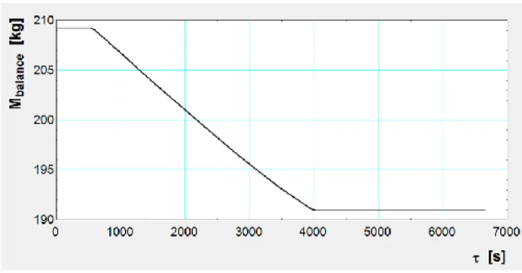
A typical curve recorded by the balance is shown in Figure 2.

Figure2: Weight of the CO2 bottles

A comparison between recorded and simulated indoor CO2 concentrations is presented in Figure 3.

Figure 3: Recorded and simulated CO2 concentrations inside the zone

The difference is explained by (still remaining) uncontrolled infiltrations and also by some remaining non-homogeneity in internal contamination (non-perfect mixing). 3.2 In an office room

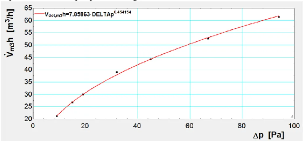
One of the air terminal unit has been calibrated in laboratory in order to identify a relationship between the air flow rate supplied to the room and the terminal pressure drop. Such relationship is plotted in Figure 4.

Figure 4: Calibration of one terminal unit

The tracer gas equipment used in this office room is presented in Figure 5.

Figure 5 : Tracer gas equipment

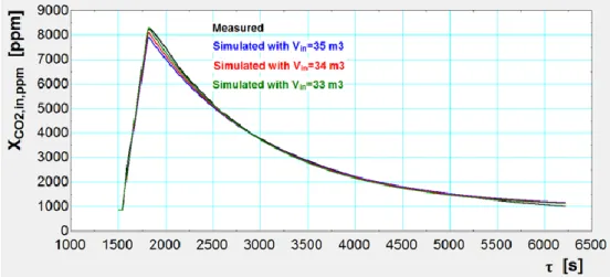
Recorded and simulated indoor air CO2 concentrations are compared in Figure 6. Several iterations are required to identify a satisfactory value of the effective volume. The best result (coincidence between the recorded and simulated peaks) is obtained with an effective volume of 33 m3.

Figure 6: measured and simulated CO2 concentrations inside the zone

4. Possibility of combination with a co-heating test 4.1 The principle

An attractive solution consists in using a small butane burner to produce heat and CO2 during a limited time and recording temperatures, CO2 and also water vapor concentrations.

The source can be, for example, a small camping cooker is equipped with a bottle of 190 g of Butane.

The total combustion of this amount of butane is producing the following emissions: (19) (20)

(21)

This corresponds to 0.5711 kg of carbon dioxide and 0.292 kg of water. The amount of energy liberated by this combustion is defined as follows:

(22) (23)

Which gives 8.534 MJ or 2.371 kWh. The combustion can be tuned in such a way to produce almost constant emissions of CO2 and heat on a pre-fixed time period. The system can be pre-calibrated by continuous weighting in such a way to define the actual emission curves to be used as inputs in the simulation.

4.2 Prospective

A first evaluation of this new approach consists in simulating the response of a real building zone. The example considered is the living room of a house which has been extensively studied in the frame of the IEA-ECB annex 58 project [2][3]. All solar protections are closed. All internal heat gains other than the butane combustion are eliminated.

Just in order to provide a better visualization of the phenomena, the cellar and the attic are supposed to be maintained at outdoor temperature.

Simulations are performed on a dozen of hours with different combustion rates, but consuming the same amount of butane (190 g).

The burner is supposed to provide constant emissions (rectangular signals).

Heat and CO2 balances are established by simulations with the model previously used [2]. In this model, the occupancy emissions are replaced by the corresponding emissions of the burner.

CO2 balance:

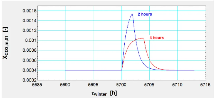
The simulated contamination of is presented in Figure 7. The two cases considered correspond to a total combustion of the C4H10 available in 2 and 4 hours respectively.

Figure 7: Simulation of the CO2 contamination

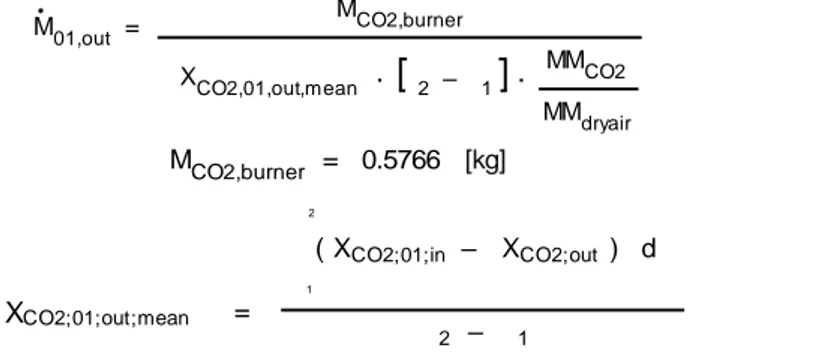
If neglecting again the transient component (initial and final contaminations are the same on the time period considered), the combination of two integrations (CO2 supply

and corresponding contamination) allows calculating the (average) ventilation flow rate: M_01,out = MCO2,burner DX_{CO2,01,out,mean} · t₂ – t1 · MM_CO2 MM_dryair (24) M_CO2,burner = 0.5766 [kg] (25) DXCO2;01;out;mean =

ò

In the case considered, the air flow rate is estimated to 14.07 and 14.02 m3/h with 2 and 4 hours of combustion time, respectively.

Heat balance:

The simulated indoor air temperatures of the two cases considered as plotted in Figure 8.

Figure 8: Living room and outdoor temperatures

Average temperatures are calculated on the period of time considered (from tau1=5695 to tau2=5715h).

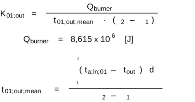
If neglecting the energy storage, the global heat transfer coefficient between the living room and the outside environment (through all the internal and external walls, including the windows and through the ventilation) can be defined as follows:

K01;out = Qburner Dt01;out;mean · (t2 – t1) (27) Qburner = 8,615x106 [J] (28) Dt01;out;mean =

ò

Which gives almost the same values, 61.01 and 60.75 W/K, with 2 and 4 hours of combustion durations respectively.

But much more should be learned by comparing simulated and measured response factors (i.e. comparing the curves of Figure 8 with measured values)…

4.3 Test in climatic room

This new method has been tested in a climatic room. Examples of results are presented in Figures 9 to 11. The three recorded “responses” of the climate room are compared to simulations. The two first comparisons (on CO2 and water vapor concentrations) are used to identify the actual air renewal. Then, the third comparison (on temperatures) can be used to tune the thermal simulation model of the room.

0 1000 2000 3000 4000 5000 6000 7000 0 500 1000 1500 2000 2500 3000 3500 4000 t [s] XCO2,in,ppm XCO2,su,ppm simulation C O 2 C o n c e n tr a ti o n [ p p m ]

0 1000 2000 3000 4000 5000 6000 7000 0.0055 0.006 0.0065 0.007 0.0075 0.008 0.0085 0.009 0.0095 0.01 t [s] w [ k g o f w a te r/ k g o f d ry a ir ] Simulation win wsu

Figure 10: Response of the climate room to the emission of water vapor produced by the butane burner

0 1000 2000 3000 4000 5000 6000 7000 10 12.5 15 17.5 20 22.5 25 27.5 30 t [s] tin tsu simulation T [ °C ]

Figure 11: Response of the climate room to the sensible heat emission produced by the butane burner

5. Conclusion

The method consisting in contaminating a building zone by direct combustion should allow identifying, not only the actual air renovation, but also the actual thermal response of this zone. It appears as a very expedient way to combine both tracer gas and co-heating procedures.

Aknowledgements

This research is financially supported by the Walloon Region of Belgium

References

[1] ASTM standard E741-00, “Standard Test Method for Determining Air Change Rate in a Single Zone by Means of a Tracer Dilution”, Philadelphia PA 2000

[2] Strachan P., I. Heusler, Empirical whole Model Validation Modelling Specification: Test case Twin_House_1, IEA ECB Annex 58 Validation of Building Energy Simulation Tools, Subtask 4, May 2014. [3] Masy G., Rehab I., André P., Georges E., Randaxhe F., Lemort V, Lebrun J. Lessons Learned from Heat Balance Analysis for Holzkirchen Twin Houses Experiment. 6th International Building Physics Conference, IBPC 2015.