Aggregation of flexible domestic heat pumps for
the provision of reserve in power systems.
E. Georges*a, S. Quoilina, S. Mathieub, V. Lemorta
a Energy Systems Research Unit, Thermodynamics Laboratory, University of Liège, Liège, Belgium,
*email: [email protected]
b
Systems and Modeling Research Unit, Department of Electrical Engineering and Computer Science, University of Liège, Liège, Belgium.
Abstract:
The integration of renewable energy sources in the electricity production mix has an important impact on the management of the electricity grid, due to their intermittency. In particular, there is a rising need for flexibility, both on the supply and demand sides. This paper assesses the amount of flexibility that could be reserved from a set of flexible residential heat pumps in a given geographical area. It addresses the problem of a load aggregator controlling a set of heat pumps used to provide both space-heating and domestic hot water. The flexibility of the heat pumps is unlocked in order to reduce electricity procurement costs in the day-ahead electricity market, while ensuring the provision of a predefined amount of reserve for real-time grid management. The objective of the paper is two-fold. On the one hand, an aggregation method of large sets of heat pumps based on physics-based models and random sampling techniques is proposed. On the other hand, a combined optimization problem is formulated to determine both the optimal electricity demand profile to be bought on the day-ahead market and the cost associated to the reservation of a defined amount of power. The method is applied to a set of 40000 residential heat pumps in Belgian houses. Results show that these houses can provide up to 100MW of upward reserve for 50% of the current costs. The provision of downward reserve at competitive cost is hampered by significant overconsumption.
Keywords:
Heat pumps, flexibility, linear optimization, ancillary services, power systems.
1. Introduction
1.1. General context
The fast spread of distributed power generation through the integration of renewable energy sources represents additional challenges for the management of the electricity grid. One main objective of this management is to ensure the balancing between electricity consumption and production. The intermittency of these renewable energies makes such balancing more difficult. Conventional power modulations on the supply-side are no longer enough to ensure security of supply, resulting in an increased need for flexibility of the demand-side. In this context, buildings can become key systems for demand-side management. Indeed, in the coming years, a substantial electrification of this sector is expected with increased use of electric/plug-in hybrid vehicles or high efficiency heat pumps. To manage all these flexible loads, a new entity, called aggregator, is being developed. The aggregator pools the flexibility of electricity consumers and can either trade it on the electricity market, or offer it as a service to electricity grid management entities. In this paper, the potential of flexible heat pumps is investigated in the context of the provision of reserve.
1.2. Load aggregation methods
As the number of flexible loads considered increases, it becomes computationally expensive to model each end-user separately. In the literature, studies that investigate large-scale flexibility of domestic thermostatically-controlled loads (TCLs) resort to aggregated models. In the study of Biegel et al. [1], an equivalent lumped first-order RC analogy is used to model the thermal behavior
of a set of heterogeneous houses. Model parameters, temperature limits and power constraints are set to the average values of the set. The authors point out the lack of accuracy that may arise from such modeling approach. Indeed, as shown by Hao et al. [2], a distinction exists between the modeling of homogeneous and heterogeneous populations of TLCs. In the case of a homogeneous population of loads, one can define a generalized battery model with a capacity equal to the average capacity of the set, and power limits set to the average over the set of loads. This is no longer exact for a set of heterogeneous loads. In that case, a sufficient condition consists in modeling the general battery with power limits and capacity corresponding to the limiting case of the population of loads. Papaefthymiou et al. [3] propose to model an aggregated set of buildings equipped with heat pumps as an equivalent storage plant. Similar loads are first pooled and modeled using detailed simulation tools. Comfort-driven simulations are performed in order to derive minimum and maximum temperature bounds, as well as power bounds for the aggregated model. In the aggregated model, temperature changes are modeled by a linear function of the heat pump electrical power variations. An aggregated model of residential buildings with heat pumps for demand side management is also proposed by Patteeuw and Helsen [4]. Each house differs by its characteristics and occupants' behavior. First, each house is modeled separately in order to determine its warm-up and cool-down temperature curves. The obtained curves are then averaged over the set of buildings and used as lower bound for the unique aggregated model. For domestic hot water, there are as many equivalent tank models as the maximum number of inhabitants. The actual lower bounds for the water storage tank temperatures are determined along with the average hot water demand. Although in line with the sufficient condition established in [2], the aggregation methods proposed in [3] and [4] still require to model each building separately in order to determine lower temperature bounds of the aggregated model. This may limit the ability of these methods to be extended to large-scale simulations, as it becomes challenging to model each building separately. In light of the above review, one objective of this paper is to develop reliable aggregated models that do not require modeling of each building a-priori.
1.3. Flexible loads for ancillary services
To ensure grid balance and security of supply, different balancing mechanisms have been established by Transmission System Operators (TSOs). Power reserves are part of these mechanisms. In Europe, one distinguishes three types of power reserves: frequency containment reserve, frequency restauration reserve and replacement reserve. Among frequency restauration reserves, one distinguishes automatic (aFRR, also known as secondary reserve) and manual (mFRR, also known as tertiary reserve) reserves. The capacities of secondary reserves must be made fully available within 30 seconds and be provided for 15 minutes. For tertiary reserves, they must be made available after 15 minutes, for an undetermined amount of time. Such reserves are used to solve regional imbalance and restore frequency. In the frame of the secondary reserve, the amount of power that must be acquired on a yearly basis is determined by TSOs. In Belgium, the TSO distinguishes two actions within the provision of secondary reserves: reservation and activation. The reservation consists in contracting the defined amount of reserve from different providers. Reserve providers inform the TSO of the amount of reserve they can provide on a quarter-hourly basis, along with the opportunity costs associated to this reservation. Indeed, such power reservation prevents the use of those assets in other market segments. One day ahead, all parties enrolled in the provision of secondary reserve can offer an extra volume of reserve for the next day. In real-time, if needed, the reserve is activated by the TSO. In the following, only the problem of power reservation is considered.
Several studies focus on the use of demand response for the provision of reserve ([5], [6] and [7]). As opposed to commercial and industrial consumers, residential demand response with TLCs is not yet implemented in this context, but offers a promising potential through direct load control by third-party aggregator ([8]). Given their fast dynamics, heat pumps, provided that they are equipped with suitable communication devices, are well-suited to provide secondary reserve. However,
Biegel et al. [9] have identified three challenges associated to the provision of reserve by such flexible consumers: energy limitations, uncertainty in the baseline consumption and risks of suboptimal market operation. The available literature on the subject is limited and based on demand-side models with little level of details. This paper investigates the problem of power reservation with residential heat pumps, with a focus on the determination of reservation costs for future integration in the reserve market.
2. Methodology
2.1. Thermal models
The thermal behaviour of buildings is modeled by an equivalent thermal network (Fig. 1) consisting of thermal resistances, R, in K/W, and lumped thermal capacitances, C in J/K. Each building is equipped with variable-speed air-to-water heat pump modeled by polynomial laws that express the coefficient of performance (COP) as a function of ambient temperature, water supply temperature, and part-load ratio. Regression coefficients are identified based on performance curve from manufacturer data. The water supply temperature is adapted to the house insulation level and adjusted throughout the year following a heating curve. DHW tanks are modeled by one-node models with homogeneous water temperature.
Fig. 1: Building grey-box model structure.
2.2. Load aggregation with random sampling
In previous work [10], a method to cluster houses according to their similarities in terms of geometrical and thermal characteristics was presented. The objective of this section is to extend the aggregation method to take into account the diversity of user consumption profiles for space-heating and domestic hot water (DHW). Indeed, the diversity of load profiles results in heterogeneous populations among similar houses of a cluster, which cannot be accurately modeled by average values. The proposed method relies on the knowledge of the following data by the load aggregator:
▪ house geometry and insulation level,
▪ heat pump nominal power and rated performance,
▪ desired temperature set point profile and allowed temperature dead band around the set point, ▪ DHW tank size,
▪ total number of occupants in the house,
▪ hot water demand profiles, based either on average historical data, or on the definition of time periods of high demand probability.
2.2.1. Aggregation of space-heating demand
To aggregate the electrical consumption associated to space-heating needs, a first option consists in averaging the temperature set points of all buildings. This results in a single aggregated model. A second method consists in associating the different profiles either to one of three conventional categories (constant, night set-back and intermittent heating schedules) or to a "random" category.
This method is referred to as quota sampling. The classification in each category is based on the measure of the integrated temperature difference between each profile and a reference profile for each category. Similarities with the four categories of profiles are established as follows:
1. determine the number of temperature levels in the profile,
2. determine the similarity of the profile with one of the three conventional profiles:
in the case of one temperature level: assign the profile to the "constant" profiles category, in the case two temperature levels: the profile could belong either to the "night set-back", or to
the "intermittent" or to the "random" category. To choose the category, equivalent night set-back (𝑇𝑡𝑛𝑠𝑏) and intermittent (𝑇
𝑡𝑖𝑛𝑡) profiles are built based on the temperature levels
determined in the first step. The profile is then compared against those two reference profiles by the average integrated temperature difference, as follows:
∆𝑛𝑠𝑏=∑ 𝑇𝑡− 𝑇𝑡 𝑛𝑠𝑏 𝑡 𝑛 (1) ∆𝑖𝑛𝑡=∑ 𝑇𝑡− 𝑇𝑡 𝑖𝑛𝑡 𝑡 𝑛 (2)
where n is the number of periods.
If the difference is larger than 1K, the profile is associated to the "random" profile category. If it is below that value, it is associated to the profile category with the minimum average integrated temperature difference.
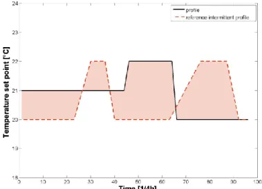
for three temperature levels: the procedure is identical to the case with two temperature levels. The category options for the profile are "intermittent" or "random". The principle is illustrated in Fig. 2.
3. once distributed among the categories, all profiles in one cluster are averaged. Corresponding upper and lower temperature bounds are derived. These aggregated profiles are then used as temperature bounds in the building model. Depending on the diversity of profiles, the number of aggregated models varies between one and four.
Fig. 2: Illustration of the method to classify temperature set point profiles. The chosen example profile has three temperature levels (black). The corresponding reference "intermittent" profile is such that the temperature is equal to the maximum temperature of the example profile during occupied periods and to the minimum temperature during unoccupied period (red). ∆𝑖𝑛𝑡 is equal to 1.23, and the profile is thus associated to the "random" category.
As proposed in [4], the accuracy of aggregated models can be determined from their ability to reproduce power profiles obtained in response to variable tariffs. The two clustering methods are applied to a set of one hundred buildings equipped with price-responsive heat pumps. First, each
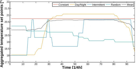
building is simulated separately in order to obtain a reference consumption profile. The aggregated electricity consumption profile is the sum of the profiles obtained for each building. Secondly, aggregated models are derived following the quota sampling method, resulting in four different clusters. Results for the set of one hundred buildings are obtained by multiplying the results obtained with each aggregated model by the number of buildings that fall in each category. Results are illustrated in Fig. 3. Figure 3a compares the aggregation of set points into four categories to the averaging into one profile (“mean”). Figure 3b shows the aggregated power consumption profile obtained with one hundred models and the results obtained with the two aggregation methods. The RMS errors on the zone temperature obtained are 0.43K and 0.09K with averaging and quota sampling methods, respectively. Corresponding normalized RMS errors on the electric power are 36.9% and 11.9%, respectively. Based on these results, it can be inferred that representing the set of buildings only with one model constrained by the average of the constraints of all the buildings results in a substantial loss of accuracy, due to the heterogeneity of the population of loads. Contrariwise, these results confirm the validity the aggregation method based on the similarity in set point constraints following the quota sampling method.
a) Set points aggregation with the averaging method (“mean”) compared to quota sampling method with four categories (constant, day/night, intermittent and random).
b) Total electrical power obtained with the averaging (1 model) and quota sampling (4 models). Fig. 3: Comparison of the power consumption profiles obtained with two aggregation methods to
those obtained with one model for each of the one hundred buildings.
0 10 20 30 40 50 60 70 80 90 17.5 18 18.5 19 19.5 20 20.5 21 21.5 22 Time [1/4h] A g g re g a te d t e m p e ra tu re s e t p o in ts [ °C ]
Constant Day/Night Intermittent Random Mean
0 10 20 30 40 50 60 70 80 90 0 0.2 0.4 0.6 0.8 1 1.2 1.4 1.6 1.8 2x 10 5 Time [1/4h] A g g re g a te d p o w e r [ W ] 100 models averaging quota sampling
2.2.2. Aggregation of domestic hot water demand
Different methods can be used to represent a cluster of domestic hot water tanks. The first method, referred to as averaging method, consists in modeling a single water tank with a volume equal to the average tank volume of the set of buildings and with the average DHW demand profile. The second method follows a random sampling technique. Such sampling methods are used when the population is very large and random. In this method, it is proposed to determine a number of representative profiles, comprised between one and five. The choice of representative profiles is carried out in several steps:
1. Hourly DHW draw-off profiles are normalized with respect to the integrated daily value.
2. In order to capture relevant patterns, DHW draw-off events of volume inferior to one-tenth of the integrated daily usage are discarded. Other normalized DHW draw-off values are set to one. 3. A pairwise comparison of all normalized profiles is performed based on the computation of the
RMS difference between them 𝑅𝑀𝑆𝐷𝑖,𝑗 = √
∑𝑛 (𝑉̇𝑖,𝑡∗ −
𝑡=1 𝑉̇𝑗,𝑡∗)2
𝑛 (3)
4. To each profile i is associated the profile j with the smallest 𝑅𝑀𝑆𝐷𝑖,𝑗. There can be more than
one possibility. The resulting correspondence matrix is reduced to a column vector by replacing profiles with identical 𝑅𝑀𝑆𝐷𝑖,𝑗 by the profile with the largest number of occurrences in the
matrix.
5. Resulting typical profiles are then ranked according to their occurrence in the vector. If there are more than five remaining profiles, the first five are chosen as representative profiles.
6. Profiles that did not fall into those five categories are redistributed in the category with the smallest RMSD.
An example of normalized representative DHW profiles obtained through the above procedure is provided. In this example, an initial set of 55 profiles is used. Five representative profiles are identified. They are compared to the average of the subset of profiles in the category in Fig. 4. Aggregated DHW use profiles are given by the average of the profiles that fall in each category. Tank volumes, contrariwise, are set to the average value over the entire set of water tanks, regardless of the identified categories.
Since heat pumps are used to supply both DHW and space heating, the validity of the proposed clustering method is verified in a combined exercise in the next section.
2.2.3 Aggregation of both space-heating and domestic hot water demands
To each subset of buildings derived from the aggregation based on space heating needs (quota sampling method) is associated one to five subsets of aggregated DHW tanks. One building model and one water tank represent the behavior of several of them. Since heat pumps are used to cover both space heating and DHW needs, this has several implications in the context of the aggregation. First, within a decision time step, the heat pump is allowed to work in both SH and DHW modes simultaneously. Secondly, the aggregation of water tanks removes the existing diversity of temperature levels and tank sizes, which tend to lead to coordinated power peaks. To mitigate this effect, it is proposed to limit the heat pump power devoted to the domestic hot water production proportionally to the number of water tanks represented by each aggregated model. The total aggregated power over the set of buildings is the weighted average sum of power profiles for space heating and DHW production obtained for each aggregated model, such that
𝑃𝑡 = ∑ ∑ (𝑊𝑖𝑗,𝑡𝑠 𝑗𝑖𝑚𝑎𝑥 𝑗=1 + 𝑊𝑖𝑗,𝑡𝑤 𝑖𝑚𝑎𝑥 𝑖=1 ) 𝛼𝑖𝑗 = ∑(𝑊𝑘,𝑡𝑠 + 𝑊𝑘,𝑡𝑤 𝑛𝑐 𝑘=1 ) 𝛼𝑘 (4)
where {1. . 𝑖𝑚𝑎𝑥} is the set of heating set-point categories, 𝑗𝑖𝑚𝑎𝑥 represents the number of models of DHW tanks for each house type i and 𝑛𝐶 is the total number of aggregated models.
The same set of one hundred buildings as in Section 2.2.1. is used to compare the two aggregation methods, i.e. averaging and random sampling of DHW demand with quota sampling of space-heating needs. RMS error on the electrical power consumption of 27.2 and 22.5% are obtained, respectively. The poorer performance of the averaging technique comes from the loss of load diversity which, despite the power limitation, results in power peaks. The random sampling method allows adapting the number of models from 4 to 20 depending on the diversity of DHW profiles.
Fig. 4: Example of normalized representative DHW profiles obtained with the proposed method for a set of 55 profiles. Comparison between representative and average profiles of the category.
2.2. Power reservation – problem statement
The amount of reserve that can be provided by a set of heat pumps is determined one day ahead by a combined optimization problem. The objective is to unlock the flexibility offered by heat pumps
to reduce electricity procurement costs in the day-ahead electricity market, while ensuring the provision of a predefined amount of reserve for real-time grid management. The optimization problem determines both the optimal electricity demand profile to be bought on the day-ahead market and the cost associated to the reservation of a given amount of power. For upward reserve, the optimization problem can be formulated as
min ∑ (∑(𝑃̂𝑖,𝑡𝛼𝑖)𝜋𝑡𝐷𝐴 𝑛𝑐 𝑖=1 ) 𝑑𝑡 + 𝛽 ∑ 𝜆𝜏 𝜏∈𝑀 𝑡∈𝐻 (5) subject to, ∀𝑖 ∈ {1, … , 𝑛𝐶}, ∀𝑡 ∈ 𝐻, 𝒙 ̂𝑖,𝑡+1 = 𝑓(𝒙̂𝑖,𝑡, 𝑊̂𝑖,𝑡𝑠, 𝑊̂𝑖,𝑡𝑤, 𝒖𝑡) (6) 𝑃̂𝑖,𝑡 = 𝑊̂𝑖,𝑡𝑠 + 𝑊̂𝑖,𝑡𝑤 + Γ𝑖,𝑡 (7) 𝒙𝑖,𝑡𝑚𝑖𝑛≤ 𝒙̂𝑖,𝑡 ≤ 𝒙𝑖,𝑡𝑚𝑎𝑥 (8) 0 ≤ 𝑊̂𝑖,𝑡𝑠 ≤ 𝑦̂𝑖,𝑡𝑊𝑖,𝑡𝑠,𝑚𝑎𝑥 (9) 0 ≤ 𝑊̂𝑖,𝑡𝑤 ≤ (1 − 𝑦̂𝑖,𝑡)𝑊𝑖,𝑡 𝑤,𝑚𝑎𝑥 (10) 0 ≤ 𝑦̂𝑖,𝑡 ≤ 1 (11) and ∀𝑖 ∈ {1, … , 𝑛𝐶}, ∀𝜏 ∈ 𝑀, ∀𝑡∗ ∈ {0, … , 𝑘}, to 𝒙𝑖,𝜏 = 𝒙̂𝑖,𝜏 (12) 𝑃𝑖,𝜏,𝑡∗ = 𝑃̂𝑖,𝜏+𝑡∗+ 𝛿𝑖,𝜏,𝑡∗ (13) 𝑃𝑖,𝜏,𝑡∗ = 𝑊𝑖,𝜏,𝑡𝑠 ∗ + 𝑊𝑖,𝜏,𝑡𝑤 ∗+ 𝛤𝑖,𝜏+𝑡∗ (14) 𝒙𝑖,𝜏,𝑡∗+1= 𝑓(𝒙𝑖,𝜏,𝑡∗, 𝑊𝑖,𝜏,𝑡𝑠 ∗, 𝑊𝑖,𝜏,𝑡𝑤 ∗, 𝒖𝑡) (15) 𝒙𝑖,𝜏+𝑡𝑚𝑖𝑛∗ ≤ 𝒙𝑖,𝜏,𝑡∗ ≤ 𝒙𝑖,𝜏+𝑡𝑚𝑎𝑥∗ (16) 0 ≤ 𝑊𝑖,𝜏,𝑡𝑠 ∗ ≤ 𝑦𝑖,𝜏,𝑡∗𝑊𝑖,𝜏,+𝑠,𝑚𝑎𝑥 (17) 0 ≤ 𝑊𝑖,𝜏,𝑡𝑤 ∗ ≤ (1 − 𝑦𝑖,𝜏,𝑡∗)𝑊 𝑖,𝜏+𝑡∗ 𝑤,𝑚𝑎𝑥 (18) 0 ≤ 𝑦𝑖,𝜏,𝑡∗ ≤ 1 (19) ∑ 𝛿𝑖,𝜏,0 𝑛𝐶 𝑖=1 𝛼𝑖 ≥ 𝑅(1 − 𝜆𝜏) (20) −𝜎 ≤ 𝒙̂𝑖,𝜏+𝑘+1− 𝒙𝑖,𝜏,𝑘+1≤ 𝜎 (21)
Houses equipped with heat pumps are aggregated in 𝑛𝐶 clusters according to the method proposed
in Section 2.1, and 𝛼𝑖 is the number of houses aggregated in each cluster i. The amount of power
bought per average house of each cluster i in period t, 𝑃̂𝑖,𝑡 at the day-ahead market price 𝜋𝑡𝐷𝐴, is defined in (7) as the sum of the heat pump consumption for space heating, 𝑊̂𝑖,𝑡𝑠, or domestic hot water heating, 𝑊̂𝑖,𝑡𝑤, and of the exogenous consumption, 𝛤𝑖,𝑡. Variable 𝑦̂𝑖,𝑡, models the fact that the heat pump can be used to supply both DHW and space heating. It is equal to one if all heat pumps in a cluster are used for space heating and equal to zero if they all produce domestic hot water. 𝑘 is the number of payback periods to allow the system to return to its baseline consumption (𝑃̂𝑖,𝑡). The
initial conditions of state variables are given by (12). Equation (13) defines the amount of power that can be reserved with respect to the baseline consumption profile. For all periods in 𝑀, a predefined amount of power 𝑅 is reserved in Equation (20). Beyond a certain value, the same amount of reserve may not be achievable for all periods. Variable 𝜆 serves the purpose of relaxing
this constraint for such periods. Finally, (21) ensures that the state at the end of the payback period is close enough to the one given by the baseline.
The case of downward reserve is obtained by replacing (20) by ∑ 𝛿𝑖,𝜏
𝑛𝐶
𝑖=1
𝛼𝑖 ≤ 𝑅(1 − 𝜆𝜏) (𝑅 ≤ 0) (22)
The cost entailed by power reservation is given by the shadow price1 of constraint (20) (resp. (22)). For these problems to remain linear, the heat pump COP is expressed as a function of the ambient temperature only. Water supply temperatures are set by the heating curve in space-heating mode, and by the maximum water temperature in DHW mode.
Finally, lower and upper temperature bounds in (16) should be set to the most restrictive values of the set ([2]), such that
𝑥𝑡𝑚𝑖𝑛 = max 𝑖∈{1…𝑖𝑚𝑎𝑥}𝑥𝑖,𝑡 𝑚𝑖𝑛 (23) 𝑥𝑡𝑚𝑎𝑥 = 𝑚𝑎𝑥 ( 𝑚𝑖𝑛 𝑖∈{1…𝑖𝑚𝑎𝑥}𝑥𝑖,𝑡 𝑚𝑎𝑥, 𝑥 𝑡𝑚𝑖𝑛) (24)
where {1. . 𝑖𝑚𝑎𝑥} is the set of heating set-point categories.
3. Results
3.1 Illustration on a single house
The modification in baseline consumption entailed by power reservation is illustrated in Figure 5 for an example house. The payback period is set to 10 periods of 15 minutes. In this example, a minimum upward power reservation of 2000 W is contracted for all periods of the day. Due to the time varying electricity tariff, the baseline consumption profile without power reservation (R+ = 0) increases during periods 25 to 30. To be able to provide upward reserve in those periods, the baseline consumption profile is modified (R+ > 0) and increases in time periods 20 to 25. This modification in baseline profile yields a suboptimal control in terms of electricity costs. The latter increase by 0.5% in this case.
Fig.5: Illustration of the influence of power reservation on baseline consumption profile.
1
3.2 Application in the Belgian context
The above power reservation problems are solved for a case-study in the Belgian context. To that end, a set of 40000 different buildings is considered. All houses are characterized by the same geometry, representative of a typical two-story freestanding house with a heavy concrete structure, and built after 1991. Two insulation levels are considered:
▪ K45-level, which corresponds the Belgian standards for newly built houses before 2014. The overall U-value is 0.46 W/m²K.
▪ K30-level, which corresponds to an overall U-value of 0.305 W/m²K.
The share of K30 and K45-level buildings is set to 25% and 75%, respectively. 40000 different daily appliances and lighting profiles, heating set point profiles and DHW demand profiles are generated from a database developed in previous work ([11]).
Optimization problem (5)-(21) is solved for several typical days with real data corresponding to year 2012. The payback is arbitrarily set to 10 periods ([12]). Reservation costs can be compared against historical data for the provision of secondary reserve ([13]). Price profiles are illustrated for a typical day in January in Fig. 6a. For upward reserve, it is possible to provide up to 115 MW at 0 to 94% of the remuneration, depending on the period of the day. Above 115 MW, prices increase quickly, especially for time periods between 0 and 8 am, and it is not possible to guarantee the same amount of reserve for all periods of the day. This increase is due to both the imposed payback period and the limited heat pump capacities. Indeed, imposing the payback period forces the system to return to its baseline state. As the amount of upward power reserve increases, thermal inertia of systems maintains higher temperature levels. This causes the baseline consumption to increase, in order to comply with the fixed payback constraint. The electricity consumption increases by 1.6% for an upward reserve of 115 MW.
The minimization of baseline costs drives the different temperature levels towards their lower bounds during time periods with high day-ahead market prices. The provision of downward reserve during those periods therefore entails significant overconsumption. As an example, the provision of 30 MW of downward reserve entails 4.1% overconsumption. Compared to other sources of reserve available on the market (R2-), it is possible to provide only around 30 MW at competitive price, as shown in Fig. 6b. The maximum amount of downward reserve that can be provided for each period of the day is around 35 MW for that particular day.
a) Upward reserve. b) Downward reserve.
Fig. 6: Reservation cost: daily profiles for January 24th, 2012. Comparison of the prices obtained with flexible heat pumps for different levels of power reserve to average historical prices
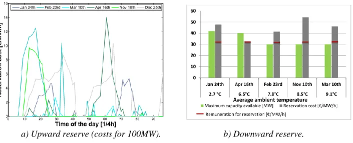
Reservation costs are presented for different days for the months of November through April in Fig. 7a for upward reserve. In all cases, an upward reserve potential of at least 100 MW can be guaranteed by the load aggregator. Resulting reservation costs range between 0 and 14 €/MWh, and are much lower than the historical remuneration for the reservation, equal to 32 €/MWh. For downward reserve, the maximum amount of reserve decreases as average daily ambient temperature increase, as shown in Fig. 7b. Most of the time however, providing the maximum amount of downward reserve is not competitive compared to current market prices.
a) Upward reserve (costs for 100MW). b) Downward reserve. Fig. 7: Power reservation for different months of the year.
In light of these results, it can be inferred that the potential of provision of downward reserve is limited. Considering the provision of both upward and downward reserves simultaneously would hamper the potential of providing upward reserve. However, the proposed method is straightforward to extend to the combined provision of upward and downward reserves.
4. Conclusion
In this paper, reliable physics-based aggregated models of heterogeneous sets of buildings for large-scale applications are developed. For space-heating power consumption only, agreement within 12% error was found. The addition of DHW consumption increases the error to 22.5%. As opposed to other methods available in the literature, the proposed method does not require the modeling of each building a-priori. In the second part of the paper, these aggregated models are used for large-scale assessment of the flexibility potential of residential heat pumps for the provision of secondary reserve. A combined optimization problem that aims at the minimization of procurement costs on the day-ahead market while ensuring a certain amount of reserve is proposed. Results for a case-study in the Belgian context show that provision of up to 70% of the current contracted amount of upward reserve can be achieved with 40000 units during the winter at less than 50% of the cost. The provision of downward reserve yields significant increase in baseline consumption, limiting the potential for downward reserve and increasing reservation costs.
Nomenclature
𝐻 Optimization horizon {1 … 𝐻} 𝑘 Number of payback periods
𝐾(𝜏, 𝑘)Payback horizon {𝜏, 𝜏 + 1 … 𝜏 + 𝑘} 𝑃 Total consumption [W]
𝑄 Heat gains [W]
𝑅 Amount of reserve allocated [W] 𝑇 Temperature [K]
𝑢 State-space model inputs
𝑊 Compressor electrical power [W] 𝑥 State variable
𝑦 Heat pump heating mode
Greek symbols
𝛼 Share of houses in a cluster 𝛿 Modulation amplitude
Γ Exogenous power consumed [W] 𝜆 Relaxation of power reservation 𝜎 Deviation tolerance from baseline
Subscripts and superscripts
𝑎𝑚𝑏 ambient 𝑔 gain 𝑖𝑛𝑡 internal 𝑙 light 𝑚 massive 𝑛 nominal 𝑠 space heating 𝑠𝑜𝑙 solar 𝑤 water 𝑧 zone Baseline variables are denoted with a “^”.
References
[1] Biegel B., Andersen P., Pedersen T.S., Nielsen K.M., Stoustrup J. and Hansen L.H., Electricity market optimization of heat pump portfolio. In: Proceedings of 2013 IEEE International Conference on Control Applications (CCA), August 2013, p. 294-301.
[2] Hao H., Sanandaji B.M., Poolla K. and Vincent T.L., A generalized battery model of a collection of thermostatically controlled loads for providing ancillary service. In: Proceedings of 2013 IEEE Allerton: 51st Annual Allerton Conference on Communication, Control, and Computing, p. 551-558.
[3] Papaefthymiou G., Hasche B. and Nabe C., Potential of heat pumps for demand side management and wind power integration in the German electricity market. IEEE Transactions on Sustainable Energy 2012; 3(4): 636-642.
[4] Patteeuw D. and Helsen L., Residential buildings with heat pumps, a verified bottom-up model for demand side management studies. In: Proceedings of 9th International Conference on System Simulation in Buildings, Dec. 2014.
[5] Ma O., Alkadi N., Cappers P., Denholm P., Dudley, J., Goli S., Hummon M., Kiliccote S., MacDonald J., Matson N. and Olsen, D., Demand response for ancillary services. IEEE Transactions on Smart Grid 2013; 4(4): 1988-1995.
[6] Heffner, G.. Loads providing ancillary services: Review of international experience. NREL, 2008.
[7] Mathieu S., Louveaux Q., Ernst D., and B. Cornélusse, A quantitative analysis of the effect of flexible loads on reserve markets. In: Proceedings of the 18th Power Systems Computation Conference, 2014.
[8] O'Dwyer C., Duignan R. and O'Malley M., Modeling demand response in the residential sector for the provision of reserves. In: 2012 IEEE Power and Energy Society General Meeting, p. 1-8.
[9] Biegel B., Westenholz M., Hansen L. H., Stoustrup J., Andersen P. and S. Harbo. Integration of flexible consumers in the ancillary service markets. Energy 2014; 67: 479–489.
[10] Gendebien S., Georges E., Bertagnolio S. and V. Lemort. Methodology to characterize a residential building stock using a bottom-up approach: a case study applied to Belgium. International Journal of Sustainable Energy Planning and Management 2015; 4: 71–88.
[11] Georges E., Gendebien S., Bertagnolio S. & Lemort, V. Modeling and simulation of the domestic energy use in Belgium following a bottom-up approach. In: Proceedings of the CLIMA 2013 11th REHVA World Congress & 8th International Conference on IAQVEC, June 2013.
[12] Georges E., Cornélusse B., Ernst D., Lemort V. & Mathieu S. Residential heat pump as flexible load for direct control service with parametrized duration and rebound effect. Applied Energy 2017; 187: 140-153. [13]Elia. Ancillary services: http://www.elia.be/en/suppliers/purchasing-categories/energy-purchases/Ancillary-services.