IMPROVING BINARY CLASSIFIER PERFORMANCE THROUGH AN INFORMED SAMPLING APPROACH AND IMPUTATION
SOROOSH GHORBANI
DÉPARTEMENT DE GÉNIE INFORMATIQUE ET GÉNIE LOGICIEL ÉCOLE POLYTECHNIQUE DE MONTRÉAL
THÈSE PRÉSENTÉE EN VUE DE L’OBTENTION DU DIPLÔME DE PHILOSOPHIÆ DOCTOR
(GÉNIE INFORMATIQUE) AVRIL 2016
c
ÉCOLE POLYTECHNIQUE DE MONTRÉAL
Cette thèse intitulée:
IMPROVING BINARY CLASSIFIER PERFORMANCE THROUGH AN INFORMED SAMPLING APPROACH AND IMPUTATION
présentée par: GHORBANI Soroosh
en vue de l’obtention du diplôme de: Philosophiæ Doctor a été dûment acceptée par le jury d’examen constitué de:
M. PESANT Gilles, Ph. D., président
M. DESMARAIS Michel C., Ph. D., membre et directeur de recherche M. ANTONIOL Giuliano, Ph. D., membre
DEDICATION
To my beloved parents Ahmad and Farasat
who introduced me the joy of reading from birth, to my loving spouse
Hanieh
for her patience, faith and unconditional love and to the memory of a great friend
ACKNOWLEDGEMENTS
It is a genuine pleasure, indeed honor, to extend my deepest gratitude to my supervisor, Prof. Michel C. Desmarais. His timely and insightful comments, meticulous scrutiny, enthusiasm and dynamism added considerably to my research experience and made an important part of this dissertation. I owe you my eternal gratitude for all I have learned from you Michel, Thank you!
I would like to thank all my lab colleagues and friends for collaborations, discussions, sug-gestions, and all the activities we did together.
On the personal side, I am very grateful to my family for their unflagging love and support throughout my life. My father and mother and also my wife, Hanieh have been, and will always be the source of strength and inspiration.
I am particularly thankful to my wife for her constant encouragement throughout my research period and for understanding all the late nights and weekends that went into finishing this thesis.
RÉSUMÉ
Au cours des deux dernières décennies, des progrès importants dans le domaine de l’appren-tissage automatique ont été réalisés grâce à des techniques d’échantillonnage. Relevons par exemple le renforcement (boosting), une technique qui assigne des poids aux observations pour améliorer l’entraînement du modèle, ainsi que la technique d’apprentissage actif qui utilise des données non étiquetées partielles pour décider dynamiquement quels cas sont les plus pertinents à demander à un oracle d’étiqueter.
Cette thèse s’inscrit dans ces recherches et présente une nouvelle technique d’échantillon-nage qui utilise l’entropie des données pour guider l’échantillond’échantillon-nage, un processus que nous appelons l’échantillonnage informé. L’idée centrale est que la fiabilité de l’estimation des paramètres d’un modèle peut dépendre de l’entropie des variables. Donc, l’adaptation du taux d’échantillonnage de variables basée sur leur entropie peut conduire à de meilleures estimations des paramètres.
Dans une série d’articles, nous étudions cette hypothèse pour trois modèles de classification, notamment Régression Logistique (LR), le modèle bayes naïf (NB) et le modèle d’arbre bayes naif (TAN—Tree Augmented Naive Bayes), en prenant une tâche de classification binaire avec une fonction d’erreur 0-1. Les résultats démontrent que l’échantillonnage d’entropie élevée (taux d’échantillonnage plus élevé pour les variables d’entropie élevée) améliore systématique-ment les performances de prédiction du classificateur TAN. Toutefois, pour les classificateurs NB et LR, les résultats ne sont pas concluants. Des améliorations sont obtenues pour seule-ment la moitié des 11 ensembles de données utilisées et souvent les améliorations proviennent de l’échantillonnage à entropie élevée, rarement de l’échantillonnage à entropie faible. Cette première expérience est reproduite dans une deuxième étude, cette fois en utilisant un contexte plus réaliste où l’entropie des variables est inconnue à priori, mais plutôt estimée avec des données initiales et où l’échantillonnage est ajusté à la volée avec les nouvelles estimation de l’entropie.
Les résultats démontrent qu’avec l’utilisation d’un ensemble de données initial de 1% du nombre total des exemplaires, qui variait de quelques centaines à environ 1000, les gains obtenus de l’étude précédente persistent pour le modèle TAN avec une amélioration moyenne de 13% dans la réduction l’erreur quadratique. Pour la même taille des semences, des amé-liorations ont également été obtenues pour le classificateur naïf bayésien par un facteur de 8% de l’entropie faible au lieu d’échantillonnage d’entropie élevée.
L’échantillonnage informé implique nécessairement des valeurs manquantes, et de nombreux classificateurs nécessitent soit l’imputation des valeurs manquantes, ou peuvent être améliorés par imputation. Par conséquent, l’imputation et l’échantillonnage informatif sont susceptibles d’être combinés dans la pratique. La question évidente est de savoir si les gains obtenus de chacun sont additifs ou s’ils se rapportent d’une manière plus complexe. Nous étudions dans un premier temps comment les méthodes d’imputation affectent la performance des classi-ficateurs puis si la combinaison de techniques d’imputation avec l’échantillonnage informé apporte des gains qui se cumulent.
Le gain de méthodes d’imputation sont d’abord étudiés isolément avec une analyse compara-tive de la performance de certains nouveaux algorithmes et d’autres algorithmes d’imputation bien connus avec l’objectif de déterminer dans quelle mesure le motif des améliorations est stable dans les classificateurs pour la classification binaire. Ici encore, les résultats montrent que les améliorations obtenues par des techniques d’imputation peuvent varier considéra-blement par modèle et aussi par taux de valeur manquante. Nous étudions également les améliorations le long d’une autre dimension qui est de savoir si le taux d’échantillonnage par enregistrement est stable ou varie. Des différences mineures, mais statistiquement significa-tives sont observées dans les résultats, montrant que cette dimension peut également affecter les performances du classificateur.
Dans une dernière étude, nous étudions empiriquement si les gains obtenus de l’échantillon-nage informé et de l’imputation sont additifs, ou s’ils se combinent d’une manière plus com-plexe. Les résultats montrent que les gains individuels de l’échantillonnage informé et d’im-putation sont du même ordre de grandeur, mais en général, ils ne sont pas une simple somme des améliorations individuelles. Il faut noter aussi que, malgré les résultats encourageants pour certaines combinaisons d’échantillonnage informées et des algorithmes d’imputation, une analyse détaillée des résultats de l’ensemble de données individuelles révèle que ces com-binaisons apportent rarement des performances supérieures aux algorithmes d’imputation ou à l’échantillonnage informé individuellement.
Les résultats de nos études fournissent une démonstration de l’efficacité de l’échantillonnage informé pour améliorer les performances de classification binaire pour le modèle TAN, mais les résultats sont plus mitigés pour NB et LR. En outre, l’échantillonnage à entropie élevée se révèle être le régime le plus bénéfique.
ABSTRACT
In the last two decades or so, some of the substantial advances in machine learning relate to sampling techniques. For example, boosting uses weighted sampling to improve model training, and active learning uses unlabeled data gathered so far to decide what are the most relevant data points to ask an oracle to label. This thesis introduces a novel sampling tech-nique that uses features entropy to guide the sampling, a process we call informed sampling. The central idea is that the reliability of model parameter learning may be more sensitive to variables that have low, or high entropy. Therefore, adapting the sampling rate of variables based on their entropy may lead to better parameter estimates.
In a series of papers, we first test this hypothesis for three classifier models, Logistic regression (LR), Naive Bayes (NB), and Tree Augmented Naive Bayes (TAN), and over a binary classifi-cation task with a 0-1 loss function. The results show that the high-entropy sampling (higher sampling rate for high entropy variables) systematically improves the prediction performance of the TAN classifier. However, for the NB and LR classifiers, the picture is more blurry. Improvements are obtained for only half of the 11 datasets used, and often the improvements come from high-entropy sampling, seldom from low-entropy sampling. This first experiment is replicated in a second study, this time using a more realistic context where the entropy of variables is unknown a priori, but instead is estimated with seed data and adjusted on the fly. Results showed that using a seed dataset of 1% of the total number of instances, which ranged from a few hundreds to around 1000, the improvements obtained from the former study hold for TAN with an average improvement of 13% in RMSE reduction. For the same seed size improvements were also obtained for the Naive Bayes classifier by a factor of 8% from low instead of high entropy sampling. Also, the pattern of improvements for LR was almost the same as obtained from the former study.
Notwithstanding that classifier improvements can be obtained through informed sampling, but that the pattern of improvements varies across the informed sampling approach and the classifier model, we further investigate how the imputation methods affect this pattern. This question is of high importance because informed sampling necessarily implies missing values, and many classifiers either require the imputation of missing values, or can be improved by imputation. Therefore imputation and informative sampling are likely to be combined in practice. The obvious question is whether the gains obtained from each are additive or if they relate in a more complex manner.
of the performance of some new and some well known imputation algorithms, with the ob-jective of determining to which extent the pattern of improvements is stable across classifiers for the binary classification and 0-1 loss function. Here too, results show that patterns of improvement of imputation algorithms can vary substantially per model and also per miss-ing value rate. We also investigate the improvements along a different dimension which is whether the rate of sampling per record is stable or varies. Minor, but statistically significant differences are observed in the results, showing that this dimension can also affect classifier performance.
In a final paper, first the levels of improvement from informed sampling are compared with those from a number of imputation techniques. Next, we empirically investigate whether the gains obtained from sampling and imputation are additive, or they combine in a more complex manner. The results show that the individual gains from informed sampling and imputation are within the same range and that combining high-entropy informed sampling with imputation brings significant gains to the classifiers’ performance, but generally, not as a simple sum of the individual improvements. It is also noteworthy that despite the encouraging results for some combinations of informed sampling and imputation algorithms, detailed analysis of individual dataset results reveals that these combinations rarely bring classification performance above the top imputation algorithms or informed sampling by themselves.
The results of our studies provide evidence of the effectiveness of informed sampling to improve the binary classification performance of the TAN model. Also, high-entropy sampling is shown to be the most preferable scheme to be conducted. This for example, in the context of Computerized Adaptive Testing, can be translated to favoring the highly uncertain questions (items of average difficulty). Variable number of items administered is another factor that should be taken into account when imputation is involved.
TABLE OF CONTENTS DEDICATION . . . iii ACKNOWLEDGEMENTS . . . iv RÉSUMÉ . . . v ABSTRACT . . . vii TABLE OF CONTENTS . . . ix
LIST OF TABLES . . . xii
LIST OF FIGURES . . . xiv
LIST OF ACRONYMS AND ABBREVIATIONS . . . xvii
LIST OF APPENDICES . . . xviii
CHAPTER 1 INTRODUCTION . . . 1
1.1 Overview and Motivations . . . 1
1.2 Research Questions and Objectives . . . 1
1.3 Summary of the Contributions . . . 3
1.4 Organization of the Dissertation . . . 3
CHAPTER 2 RELATED WORK . . . 5
2.1 Planned Missing Data Designs . . . 5
2.1.1 Multiple Matrix Sampling . . . 5
2.1.2 Three-Form Design (And Variations) . . . 6
2.1.3 Growth-Curve Planned Missing . . . 7
2.1.4 Monotonic Sample Reduction . . . 8
2.2 Active Learning . . . 9
2.2.1 Scenarios for Active Learning . . . 10
2.3 Dealing with Missing Values in Classification Tasks . . . 13
2.3.1 Case Deletion . . . 14
2.3.2 Imputation . . . 14
CHAPTER 3 SELECTIVE SAMPLING DESIGNS TO IMPROVE THE
PERFOR-MANCE OF CLASSIFICATION METHODS . . . 15
3.1 Chapter Overview . . . 15
3.2 Entropy . . . 16
3.3 Models . . . 16
3.3.1 Naive Bayes . . . 16
3.3.2 Logistic Regression . . . 17
3.3.3 Tree Augmented Naive Bayes (TAN) . . . 17
3.4 Experimental Methodology . . . 18
3.4.1 Entropy-based heuristic for Selective Sampling . . . 18
3.4.2 The Process . . . 19
3.4.3 Datasets . . . 19
3.5 Results . . . 20
3.6 Conclusion . . . 23
CHAPTER 4 AN ADAPTIVE SAMPLING ALGORITHM TO IMPROVE THE PER-FORMANCE OF CLASSIFICATION MODELS . . . 24
4.1 Chapter Overview . . . 24
4.2 Adaptive Sampling . . . 24
4.3 Methodology . . . 25
4.3.1 Adaptive Sampling and Seed Data . . . 25
4.3.2 Non-adaptive Selective Sampling . . . 26
4.3.3 Simulation Process . . . 26
4.4 Results . . . 26
4.5 Conclusion . . . 29
CHAPTER 5 PERFORMANCE COMPARISON OF RECENT IMPUTATION METH-ODS FOR CLASSIFICATION TASKS OVER BINARY DATA . . . 31
5.1 Chapter Overview . . . 31
5.2 Related work . . . 33
5.3 Description of Investigated Approaches . . . 35
5.3.1 The Nature of Missing Data . . . 35
5.3.2 Imputation Methods . . . 36
5.3.3 Classifier Models . . . 39
5.4 Experimental Methodology . . . 40
5.4.1 Datasets . . . 40
5.5 Results . . . 42
5.6 Conclusion . . . 46
CHAPTER 6 IMPACT OF FIXED VS. VARIABLE SAMPLING RATE PER RECORD OVER THE PERFORMANCE OF IMPUTATION METHODS IN CLASSIFICA-TION TASKS . . . 49
6.1 Chapter Overview . . . 49
6.2 Description of the Imputation Methods and the Classifiers . . . 50
6.3 Experimental Methodology . . . 50
6.3.1 Rate and Distribution of Missing Values . . . 51
6.3.2 Experimental Setup . . . 51
6.4 Results . . . 52
6.5 Conclusion . . . 57
CHAPTER 7 INFORMED SAMPLING AND IMPUTATION METHODS IN BINARY CLASSIFICATION TASKS . . . 59 7.1 Chapter Overview . . . 59 7.2 Methodology . . . 59 7.2.1 Experimental Setup . . . 60 7.3 Results . . . 62 7.3.1 First Experiment . . . 62 7.3.2 Second Experiment . . . 64 7.3.3 Detailed results . . . 67 7.4 Conclusion . . . 68
CHAPTER 8 CONCLUSION AND RESEARCH PERSPECTIVES . . . 73
8.1 Conclusion . . . 73
8.2 Limitations and Threats to Validity . . . 76
8.2.1 Generalizability . . . 76
8.3 Future Work . . . 77
REFERENCES . . . 79
LIST OF TABLES
Table 2.1 Missing data pattern for a Three-Form design . . . 7
Table 2.2 Missing data patterns for all combinations of one or two time points missing with 250 Subjects. Adapted from (Palmer and Royall, 2010) . 8 Table 2.3 An Example of Monotonic Sample Reduction . . . 9
Table 3.1 Datasets - The Mean, Minimum and Maximum of the attribute entropies have been listed . . . 20
Table 3.2 Performance comparison for the different techniques under the differ-ent schemes of sampling for Ketoprostaglandin-f1-alpha dataset (ICI-Incorrectly Classified Items and RMSE-Root-Means-Squared-Error) . 21 Table 3.3 Results of running a paired t-test on the obtained results of 100 folds based on average Pct. ICI . . . 22
Table 3.4 Results of running a paired t-test on the obtained results of 100 folds based on average RMSE . . . 22
Table 3.5 Percent of datasets on which Selective Sampling classification perfor-mance results are better (p<0.05) than Scheme 1 . . . 22
Table 3.6 Percent of datasets on which Scheme 1 classification performance re-sults are better (p<0.05) than Scheme 2, Scheme 3 or both of them . . . 23
Table 4.1 Performance comparison for the different techniques under the different schemes of sampling for Brain Chemistry dataset (ICI-Incorrectly Clas-sified Items and RMSE-Root-Means-Squared-Error) where seed dataset size=8 . . . 27
Table 4.2 RMSE difference between scheme 1 and the two other schemes for Brain Chemistry dataset. Student-t test is based on 100 random sample simulations . . . 28
Table 4.3 Number of datasets which show significant greater error (ARMSE) for each technique, under different sampling schemes, over 11 differ-ent datasets, and for differdiffer-ent seed dataset sizes . . . 29
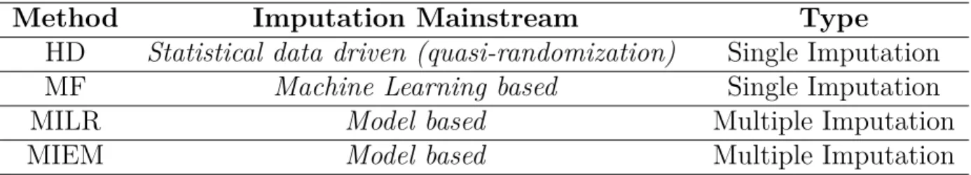
Table 5.1 Imputation Methods Used in This Study . . . 36
Table 5.2 Classifiers Considered in the Study. . . 39
Table 5.3 Datasets at a Glance. . . 40
Table 5.4 Percent of all the datasets on which applying the method improves the classification accuracy of the classifiers. . . 44
Table 7.1 Average F-Scores of NB classifier under different imputation/informed sampling methods over each dataset (Averaged over 100 Runs) . . . 68 Table 7.2 Average F-Scores of LR classifier under different imputation/informed sampling
methods over each dataset (Averaged over 100 Runs) . . . 69 Table 7.3 Average F-Scores of TAN classifier under different imputation/informed sampling
methods over each dataset (Averaged over 100 Runs) . . . 69 Table A.1 Datasets on which the mean accuracies of the classifiers (over 10 runs and 6 missing
rates) on imputed and non-imputed data are significantly different at p < 0.05. . 84 Table A.2 Datasets on which the mean accuracies of the classifiers (over 10 runs) on imputed
and non-imputed data are significantly different at p < 0.05. . . . 85 Table A.3 Datasets on which none of the imputation methods improves the classification
LIST OF FIGURES
Figure 1.1 The Thesis at a Glance. LE.S and HE.S are respectively low and high entropy sampling schemes, whereas U.S is uniform sampling as ex-plained in Chapter 3. The terms single and multiple imputation are introduced in Chapter 5 and more information on Fixed vs. Variable
rate sampling is given in Chapter 6 . . . 2
Figure 2.1 Multiple Matrix Sampling: dividing the interview questionnaire into sections of questions (shown in green) and then administering these sections to sub-samples of the main sample . . . 6
Figure 2.2 Query Synthesis. Source: (Settles, 2012) . . . 10
Figure 2.3 A handwriting recognition problem for which Query Synthesis works poorly when a human oracle is used. Source: (Settles, 2012) . . . 11
Figure 2.4 Stream-Based Selective Sampling. Source: (Settles, 2012) . . . 12
Figure 2.5 Pool-Based Sampling. Source: (Settles, 2012) . . . 13
Figure 3.1 The Binary Entropy Function (MacKay, 2003) . . . 16
Figure 3.2 a) Naive Bayes Classifier Structure and b) TAN Classifier Structure . 18 Figure 3.3 Sampling probability distribution used for the schemes 2 and 3 . . . 19
Figure 3.4 Ketoprostaglandin-f1-alpha Dataset . . . 21
Figure 4.1 Adaptive Sampling Algorithm . . . 25
Figure 4.2 Brain Chemistry Dataset . . . 27
Figure 5.1 Main Steps in Multiple Imputation (here, m is assumed to be 3). . . . 38
Figure 5.2 The General Procedure of the Experiments. . . 41
Figure 5.3 Comparison between Different Imputation Methods (Averaged over the 4 classifiers on all the datasets). . . 42
Figure 5.4 Classification Improvement for the Logistic Regression (top left), Tree Augmented Naïve Bayes (top right), Naïve Bayes (bottom left), and SVM with RBF Kernel (bottom right). . . 45
Figure 5.5 The plots represent the distribution of paired differences between the classification accuracy using each of the imputation methods and directly applying the data with missing values for each classifier. . . 47
Figure 6.1 Experimental Procedure. . . 52
Figure 6.2 Average classification accuracy of the models under different imputa-tion methods over fixed vs. variable sampling schemes(averaged over the 14 datasets and 100 runs). . . 53
Figure 6.3 Orange) percentage of datasets on which the accuracy of a given model under a given imputation method over the variable sampling scheme is significantly higher than its accuracy under the same imputation method over the fixed scheme. Blue) similarly, shows the same percentage for the fixed sampling scheme against the variable scheme (Based on one tailed Wilcoxon Signed-Rank test at p < 0.05). . . 54 Figure 6.4 Inconsistent patterns of imputation results over fixed vs. variable sampling for: A)
LR over dataset D10 at missing rate 30% and B) TAN over dataset D13 at missing rate 10%. . . 56 Figure 6.5 Percentage of datasets for which imputation results in inconsistent patterns of
ef-fects over variable vs. fixed sampling for each classifier. . . 57 Figure 7.1 Comparison. Experimental Setup. LE.S and HE.S are respectively low and high
entropy sampling schemes, whereas U.S is the uninformed, uniform sampling which is used for the imputation methods. The performance of the different classifiers over the resulting datasets is then compared . . . 60 Figure 7.2 Combination Experimental Setup. The imputation methods are applied on the
three samples created by HE.S, LE.S and U.S schemes. The performance of the different classifiers over the resulting datasets is then compared . . . 61 Figure 7.3 The Average gain (loss) in error reduction using formula (7.2) over 14 datasets and
100 runs. High entropy sampling can provide the TAN model with a substantial performance improvement that is comparable to imputation methods (HD, MF and MIEM). However, no gain is obtained for NB, and for the LR model two imputation methods bring substantial improvements (HD and MIEM) . . . 63 Figure 7.4 Results of Wilcoxon signed-rank test score improvements for individual datasets
at p < 0.05. Orange bars show the percentage of datasets on which F.Scorei >
F.Scorebase and the blue bars show the percentage of cases on which F.Scorei <
F.Scorebase where i ∈ {HD, M F, M ILR, M IEM, LE.S, HE.S} . . . 64
Figure 7.5 The average gain over imputation, GainI (eq. 7.3), when the informed sampling
and imputation are applied in tandem. For NB, high entropy sampling scheme with MILR results in an average GainI of 38%. For LR, when HE.S scheme is
coupled with MILR or MIEM an average GainI of 18.5% or 1.1% can be obtained
respectively. Finally, for TAN, HE.S with MF, MILR and MIEM brings the average
Figure 7.6 Results of Wilcoxon signed-rank test score improvements for individual datasets at p < 0.05. Orange bars show the percentage of datasets on which a signifi-cant difference is found for F.Scores,i > F.ScoreU.S,i and the blue bars show
the percentage of cases on which F.Scores,i < F.ScoreU.S,i where where i ∈
{HD, M F, M ILR, M IEM } and s ∈ {LE.S, HE.S} . . . 66 Figure 7.7 Individual dataset logit of F-scores for NB. Bars are shown relative to the baseline 70 Figure 7.8 Individual dataset logit of F-scores for LR. Bars are shown relative to the baseline 71 Figure 7.9 Individual dataset logit of F-scores for TAN. Bars are shown relative to the baseline 72
LIST OF ACRONYMS AND ABBREVIATIONS
AANN Auto-Associative Neural Networks ARMSE Average Root Mean Square Error CART Classification And Regression Tree CAT Computerized Adaptive Testing DF Degree of Freedom
DF Degrees of Freedom EC Event Covering
EM Expectation Maximization
GRNN Generalized Regression Neural Network
HD Hot deck
HE.S High Entropy Sampling ICI Incorrectly Classified Items K-NN K-Nearest Neighbors LE.S Low Entropy Sampling LR Logistic Regression MAR Missing at Random
MCAR Missing Completely at Random MF missForest
MICE Multivariate Imputation by Chained Equations
MIEM Multiple Imputation Based on Expectation Maximization MILR Multiple Imputation Based on Logistic Regression
MLE Maximum Likelihood Estimation MLP Multilayer Perceptron
NB Naive Bayes
NMAR Not Missing at Random RBF Radial Basis Function
RBFN Radial Basis Function Network RMSE Root Mean Square Error SOM Self-Organizing Map SVM Support Vector Machine TAN Tree Augmented Naive Bayes U.S Uniform Sampling
LIST OF APPENDICES
CHAPTER 1 INTRODUCTION
1.1 Overview and Motivations
Contrary to the old adage that the best solution to missing data is not to have them (Gra-ham, 2009), there are times when wisely managing or building missing data into the overall measurement design is the best use of limited resources. In some context, we can choose to allocate the observations differently among the variables during the data gathering phase, such as training a model to perform Computerized Adaptive Testing (CAT). For adaptive testing, we have the opportunity to decide upon a specific scheme of missing values for each item. We can decide which subset of questions we wish to administer to each examinee during the data gathering phase, leaving unanswered items as missing values. Recommender systems, where initial suggestions provide seed data to construct the user profile, is another example.
Given a fixed number of observations, we need to determine which variables are most critical (the most relevant information) and, potentially, ought to be allotted more observations and this leads us to optimizing the choice of missing values distribution through conducting an informed sampling process.
1.2 Research Questions and Objectives
We formalize our objectives through some concise research questions as follows:
• RQ1- Can a selective sampling approach based on uncertainty improve the performance of classifiers?
• RQ2- Can we guide the selective sampling approach on the fly, during the data gath-ering phase?
Informed selective sampling necessarily involves missing values and an obvious way to manage them is through imputation. Our study of informed sampling focuses on fixed sampling rate, since we would typically use informed sampling in a context where we have a fixed number of observations per record, or at least this is a plausible constraint in many contexts such as CAT or recommender systems as mentioned above. However the literature to date reports results of imputation techniques that use a variable rate of sampling (each record may contain
a different number of observations) for relatively small amounts of missing data. This leads to the following research question:
• RQ3- Can imputation techniques improve the prediction accuracy of classification tasks with a fixed rate of observations per record?
If the answer to the question above is positive, two more research questions can be stated as follows:
• RQ4- What is the impact of variable vs. fixed sampling rate per record on the perfor-mance of imputation methods in classification tasks?
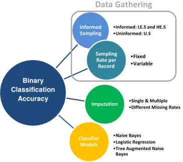
• RQ5- Are the improvements from informed sampling and from imputation additive? To address the questions above, this study revolves around improving the binary classification accuracy, as shown by figure 1.1. We explore the space created by the dimensions shown to investigate the effect of each dimension on classification performance, in particular to find out if the effect found in one dimension is independent of the others, or if they interact in a more complex way.
Informed Sampling
•Informed: LE.S and HE.S •Uninformed: U.S
Imputation •Single & Multiple •Different Missing Rates Sampling Rate per Record •Fixed •Variable Classifier Models •Naive Bayes •Logistic Regression •Tree Augmented Naive
Bayes
Binary Classification
Accuracy
Data Gathering
Figure 1.1 The Thesis at a Glance. LE.S and HE.S are respectively low and high entropy sampling schemes, whereas U.S is uniform sampling as explained in Chapter 3. The terms single and multiple imputation are introduced in Chapter 5 and more information on Fixed vs. Variable rate sampling is given in Chapter 6
1.3 Summary of the Contributions
The research presented in this dissertation has led to our main contributions listed as follows: 1. An entropy-based selective sampling design to improve the performance of classification
models (Answering research question RQ1)
2. A demonstration that the gains from the proposed informed sampling approach are maintained when entropy is estimated on the fly (Answering research question RQ2) 3. An extensive assessment of the impact of imputation methods under different sampling
schemes that resulted in the following demonstrations (Answering research questions RQ3 and RQ4):
• Imputation can improve the performance of classifiers over data with fixed rate and high proportions of missing values per record
• The choice of the rate of sampling per record between fixed and variable affects the performance of imputation methods
4. A comprehensive study on the potential additive effects of informed sampling and impu-tation methods on classification performance resulted in (Answering research questions RQ5) :
• Showing that individual gains from informed sampling and imputation are within the same range
• Demonstrating that the informed sampling often improves imputation algorithms performance, but in general the gains from the two are not additive
1.4 Organization of the Dissertation
The remainder of this dissertation provides the following content:
• Chapter 2: Presents the necessary background and introduces the related work rele-vant to this research.
• Chapter 3: Describes our proposed selective sampling approach which relies on fea-tures’ uncertainty to improve the prediction performance of binary classification. The study investigates the effect of some entropy-based sampling schemes on the predic-tive performance of three different classification models namely, Naive Bayes, Logistic Regression and Tree Augmented Naive Bayes.
• Chapter 4: Presents another study in which we further explore the entropy-based heuristic to guide the sampling process on the fly. The same sampling schemes and classification models as mentioned above are used in this study.
• Chapter 5: Explains our study which evaluates the effect of two recently proposed im-putation methods, namely missForest and Multiple Imim-putation based on Expectation-Maximization, and further investigates the effectiveness of two other imputation meth-ods: Sequential Hot-deck and multiple imputation based on Logistic Regression on data with fixed rate of missing values per record. Their effect is assessed over the classifica-tion accuracy of four different models of classifiers with respect to varying amounts of missing data (i.e., between 5% and 50%).
• Chapter 6: Presents our study which has been done again in the context of impu-tation for classification purposes and investigates whether, and how the performance of different classifiers is affected by the two sampling schemes: fixed and variable rate of observations per record given equal number of observations in total. Three single imputation methods including Mean, missForest and Sequential Hot-deck, and 2 mul-tiple imputation methods based on Logistic Regression and Expectation-Maximization are tested at 4 different amounts of missing data (ranging from 10% to 70%) with 3 different classifier models.
• Chapter 7: Demonstrates another study in which we investigate the possibility of combining the improvements (of classification prediction performance) from the in-formed sampling approach and different methods of missing values imputation. The same sampling schemes and the classification models explained in Chapter 3 are tested with the same imputation methods introduced in Chapter 5.
• Chapter 8: Presents the conclusion of this dissertation and outlines some directions of future research.
CHAPTER 2 RELATED WORK
In this chapter, we discuss relevant notable work to our research. Three main topics have been selected for the literature review. First, in section 2.1, the Planned Missing Data strategy and some of its different designs are briefly explained. Then in section 2.2, the paradigm of Active Learning is introduced and finally, in section 2.3, different approaches to deal with missing values in classification tasks are overviewed.
2.1 Planned Missing Data Designs
Selective Sampling is analogous to the notion of planned missing data designs used in psy-chometry and other domains. In planned missing data designs, participants are randomly assigned to conditions in which they do not respond to all items. Planned missing data is desirable when, for example:
• long assessments can reduce data quality, a situation that arises frequently when data is gathered from a human subject or some source for which a measurement has an effect on posterior measurements due to fatigue or boredom for example,
• data collection is time and cost intensive, and time/cost varies across attributes, in which case finding the optimal ratio of missing values over observation for each attribute is important.
Planned missing values were originally studied in the context of sampling theory and infer-ential statistics, but the issues are very similar to the ones found in the context of training a classifier, and in statistical learning algorithms in general. The data gathering phase of the learning algorithms may be faced with the same constraints as found in experimental design. Therefore, in this section, we briefly take a look at some planned missing data techniques applied in Cross-Sectional or Longitudinal studies.
2.1.1 Multiple Matrix Sampling
Multiple matrix sampling is one of the proposed methods to decrease the length of a given interview. This would involve dividing the interview questionnaire into sections of questions and then administering these sections to subsamples of the main sample, as figure 2.1 shows. It is assumed that the N items are a random sample from a population of items (just as M
participants are a random sample from a population) (Shoemaker, 1971). The most important gain in this procedure is that individuals are tested on only a portion of the test items in the total pool, and yet the parameters of the universe scores (mean of test score, variance of test score) can be accurately estimated. There are some considerations to be made in the applications of the multiple matrices sampling. These include: the number of subsets, the number of items per subset and the number of examinees administered each subset. These variables can be manipulated to create several multiple matrix sampling plans. The design to be adopted by the test developer will depend on the situations on the ground. These may be in the form of the number of available examinees, times available and the cost of materials. Several types of matrix sampling have been proposed (Anigbo, 2011).
Figure 2.1 Multiple Matrix Sampling: dividing the interview questionnaire into sections of questions (shown in green) and then administering these sections to sub-samples of the main sample
2.1.2 Three-Form Design (And Variations)
In many research contexts the number of survey items can be excessive and overburden the respondent. The Three-Form design proposed by Graham et al. (1996, 2006) is a way to overcome this dilemma. This design creates three questionnaire forms, each of which is missing a different subset of items. The design divides the item pool into four sets (Common Set X, Set A, Set B, and Set C) and allocates these sets across three questionnaire forms, such that each form includes X and is missing A, B, or C. A layout of the basic design can be found in table 2.1. As an illustration of the 3-form design, suppose a researcher is interested in administering four questionnaires to a sample of sixth graders and each questionnaire has 30 items. The resulting questionnaire battery would include 120 items. The attention span required to respond to the entire questionnaire set would be too great for a sixth grader,
but the students could realistically respond to a shorter questionnaire with 90 items. Using the 3-form design, each sixth grader will only be required to respond to 90 items, but the researcher will be able to analyze the data based on the entire set of 120 items. The 3-form design is flexible and can be adapted to research needs. However, it requires careful planning as there are a number of important nuances in implementation (e.g., optimizing power by properly allocating questionnaires to the forms, constructing the forms in a way that allows for the estimation of interactive effect) (Baraldi and Enders, 2010). Also, Graham et al. (2001) describe variations of the 3-form design that can be applied to longitudinal studies. The basic idea is to split the sample into a number of random subgroups and impose planned missing data patterns, such that each subgroup misses a particular wave (or waves) of data. The idea of purposefully introducing missing data is often met with skepticism, but they show that planned missing data designs can be more powerful than complete-data design that use the same number of data points. Graham et al.’s results suggest that collecting complete data from N participants will actually yield less power than collecting incomplete data from a larger number of respondents (Baraldi and Enders, 2010).
Table 2.1 Missing data pattern for a Three-Form design
Form Common Set X Set A Set B Set C
1 25% of items 25% of items 25% of items missing 2 25% of items 25% of items missing 25% of items 3 25% of items missing 25% of items 25% of items
2.1.3 Growth-Curve Planned Missing
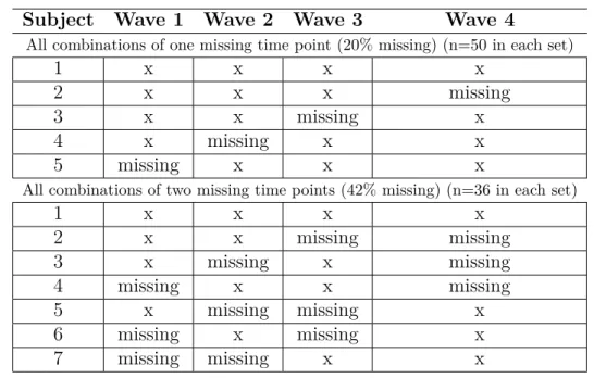
By planning the missing data pattern across subjects, the surprising usefulness of using growth curve models has been demonstrated as one solution to the problem of respondent burden in ongoing longitudinal assessments (Graham et al., 2001). A growth curve is an empirical model of the evolution of a quantity over time. In growth-curve designs, the most important parameters are the growth parameters (e.g., estimate the steepness and the shape of the curve) and estimation precision depends heavily on the first and last time points. A planned missing design can take advantage of this by putting missingness in the middle. As an example, if 250 subjects were recruited for four waves of measurement, there could be five patterns of planned missing data. One set of 50 subjects would be assessed at all waves, another set of 50 subjects would miss the first follow-up but have data on subsequent waves, another 50 would be missing only at the second follow-up, and so forth. This scenario
would yield 20% missing data. In a planned missing scenario in which subjects miss two assessment points, missing data would be 40%. Table 2.2 shows the scenario for all possible combinations of missing data points for one and then two time points with the data missing by design (Palmer and Royall, 2010).
Furthermore, Graham et al showed that, despite identical costs, a planned missing design with 30% missing data had smaller standard errors (greater power to detect an effect) than the complete case design (Graham et al., 2001).
Table 2.2 Missing data patterns for all combinations of one or two time points missing with 250 Subjects. Adapted from (Palmer and Royall, 2010)
Subject Wave 1 Wave 2 Wave 3 Wave 4
All combinations of one missing time point (20% missing) (n=50 in each set)
1 x x x x
2 x x x missing
3 x x missing x
4 x missing x x
5 missing x x x
All combinations of two missing time points (42% missing) (n=36 in each set)
1 x x x x 2 x x missing missing 3 x missing x missing 4 missing x x missing 5 x missing missing x 6 missing x missing x 7 missing missing x x
2.1.4 Monotonic Sample Reduction
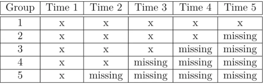
Monotonic sample reduction is sometimes used in large datasets (e.g., Early Childhood Longi-tudinal Study) to reduce costs. At each wave of measurement, a randomly-selected subgroup of the original sample is observed again. The remainder of the original participants does not need to be kept track of (treated as missing data) as table 2.3 shows. The main advantages of the approach are remarkable cost reduction and a lot of power to estimate effects that it yields at earlier waves.
Table 2.3 An Example of Monotonic Sample Reduction Group Time 1 Time 2 Time 3 Time 4 Time 5
1 x x x x x
2 x x x x missing
3 x x x missing missing
4 x x missing missing missing
5 x missing missing missing missing
2.2 Active Learning
Another close discipline to the informed sampling we study in this research is Active Learning. As a sub-field of machine learning, active learning is the study of computer systems that improve with experience and training. An active learning system develops and tests new hypotheses as part of a continuing, interactive learning process. It may ask queries, usually in the form of unlabeled data instances to be labeled by an oracle (e.g., a human annotator). For this reason, active learning is sometimes called “query learning” in the computational learning theory literature (Settles, 2012).
Having the learner ask questions or be more involved in its own training process can be very advantageous in many application contexts. For any supervised learning system to perform well, it must often be trained on hundreds (even thousands) of labeled instances. Sometimes these labels come at little or no cost through crowdsourcing, for example, the “spam” flag we mark on unwanted email messages, or the five-star rating we might give to movies on a website. Learning systems use these flags and ratings to better filter our junk email and suggest movies we might enjoy. In these examples we provide such labels for free, but we can find many other supervised learning tasks for which labeled instances are very difficult, time-consuming, or expensive to obtain. For one example, learning to classify documents or any other kind of media usually requires people to annotate each item with particular labels, such as relevant or not-relevant. Unlabeled instances are abundant from resources like the Internet, but annotating thousands of these instances can be long and tiresome and even redundant. In examples like this, data collection for traditional supervised learning systems can be very costly in terms of human effort and/or laboratory materials. If an active learning system is allowed to be part of the data collection process, where labeled data is scarce and unlabeled data abundant, it attempts to overcome the labeling bottleneck by adaptively requesting labels. In this way, the active learner aims to attain good generalization and achieve high accuracy using as few labeled instances as possible (Settles, 2010, 2012). Therefore, active learning is most appropriate when the unlabeled data instances are
numer-ous, can be easily collected, and we anticipate having to label many of them to train an accurate system.
2.2.1 Scenarios for Active Learning
The learner may be able to ask queries in several different ways. The main scenarios that have been considered for active learning in the literature are as follows (Settles, 2012):
Query Synthesis
In this setting, for any unlabeled data instance in the input space as shown in figure1 2.2, the learner may request “label membership” including queries that the learner synthesizes de novo. The only assumption is that the learner has a definition of the input space (i.e., the feature dimensions and ranges) available to it.
Figure 2.2 Query Synthesis. Source: (Settles, 2012)
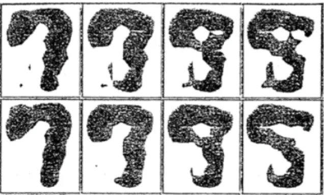
As, for instance, shown in (King et al., 2004, 2009), query synthesis is reasonable for some real-world problems, but labeling such arbitrary instances can be awkward and sometimes troublesome. Figure 2.3 shows an unexpected problem Baum and Lang (1992) encountered when they tried to use membership query learning with human oracles to train a neural network to classify handwritten characters: many of the query images generated by the
learner were merely artificial hybrid characters and not recognizable. As can be seen it is not clear what the image in the upper-right hand corner is, a 5, an 8, or a 9?
Figure 2.3 A handwriting recognition problem for which Query Synthesis works poorly when a human oracle is used. Source: (Settles, 2012)
Stream-Based Selective Sampling
In this scenario, it is assumed that obtaining an unlabeled instance is free (or inexpensive), so as illustrated by figure 2.4, it can first be sampled (typically one at a time) from the actual distribution, and then the learner can decide whether to request its label or discard it. This can be implemented in several ways. One approach can be to define a measure of utility (or information content), such that instances with higher utility are more likely to be queried (see e.g., (Dagan and Engelson, 1995)). More details on this approach and some others can be found in (Settles, 2012).
The stream-based active learning has been studied in several real-world tasks, including part-of speech tagging (Dagan and Engelson, 1995), sensor scheduling (Krishnamurthy, 2002), learning ranking functions for information retrieval (Yu, 2005) and word sense disambiguation in Japanese language (Fujii et al., 1998).
Pool-Based Sampling
As shown by figure 2.5, this scenario assumes that there is a small set of labeled data and a large pool of unlabeled data available. Queries are typically chosen in a greedy fashion from the pool, which is usually assumed to be non-changing, in accordance with a utility measure used to evaluate all instances in the pool (or a sub-sample of it in case it is very large).
Figure 2.4 Stream-Based Selective Sampling. Source: (Settles, 2012)
This scenario has been studied for many real-world problem domains in machine learning, such as text classification (Lewis and Gale, 1994), information extraction (Settles and Craven, 2008), image classification and retrieval (Zhang and Chen, 2002) and speech recognition (Tur et al., 2005), to name only a few. In fact, compared to query synthesis and stream-based scenarios which are more common in the theoretical literature, pool-based sampling is the most popular scenario for applied research in active learning (Settles, 2012).
The main difference between stream-based and pool-based active learning strategies is that the former as mentioned earlier, obtains one instance at a time sequentially, and makes each query decision individually. On the contrary, pool-based active learning evaluates and ranks the entire U before selecting the best query (Settles, 2012).
Although, the informed sampling we study in this dissertation and active learning are similar in that they both affect the training set through collecting more informative data to be used in the learning process, the strategies they use to achieve this goal is completely different: informed sampling focuses on variables (by allotting more observations to the more relevant variables) and active learning concentrates on instances (by asking the oracle to label the most informative instances). The other differences between the two are:
Figure 2.5 Pool-Based Sampling. Source: (Settles, 2012)
contexts in which active learning applies.
• Availability of abundant (unlabeled) data instances, as the main underlying assumption, is a necessity for active learning. Remembering the aforementioned CAT example, informed sampling does not have such prerequisite.
Because missing values are necessarily involved in informed sampling, we briefly look at the different strategies used in the literature to deal with missing values in the following section.
2.3 Dealing with Missing Values in Classification Tasks
Learning, inference, and prediction in the presence of missing values are pervasive problems in machine learning and statistical data analysis. The classification setting is particularly affected by the problem since many classifier models have no natural ability to deal with missing input features. Besides, missing values in either the training set or test set or in both sets affect the prediction accuracy of learned classifiers (Luengo et al., 2012). The appropriate way to handle incomplete input data depends in most cases on how data attributes became missing (three different mechanisms, which lead to the introduction of missing values are discussed in Chapter 5). Usually, the treatment of missing values in data mining can be handled in the following different ways (Luengo et al., 2012; García-Laencina et al., 2010).
2.3.1 Case Deletion
Case deletion is known as complete case analysis. It is available in all statistical packages and is the default method in many programs. This method discards all instances (cases) with missing values for at least one feature from the dataset. A variation of this method consists of determining the extent of missing data on each instance and feature, and delete the instances and/or features with high levels of missing data. Before deleting any feature, it is necessary to evaluate its relevance to the analysis. Relevant attributes should be kept even with a high degree of missing values.
Nevertheless, deletion methods are practical only when the data contain relatively small num-ber of instances with missing values and when the analysis of the remaining data (complete instances in case deletion) will not lead to serious bias during the inference.
2.3.2 Imputation
The imputation of missing values is a class of procedures that aims to substitute the missing data with estimated values. Different approaches to the imputation of missing values are introduced in Chapter 5.
2.3.3 Some Machine Learning Approaches
Using machine learning techniques, some approaches have been proposed for handling miss-ing data in classification problems avoidmiss-ing explicit imputations. In these approaches missmiss-ing values are incorporated to the classifier. Treating missing values as a separate value, decision trees like C4.5 and CART were among the first algorithms to incorporate the handling of missing data into the algorithm itself (Quinlan, 1993; Breiman et al., 1984). Neural network ensemble models and also fuzzy approaches are other examples. For more detailed informa-tion on these algorithms we refer the reader to (García-Laencina et al., 2010; Breiman et al., 1984; Quinlan, 1993).
CHAPTER 3 SELECTIVE SAMPLING DESIGNS TO IMPROVE THE PERFORMANCE OF CLASSIFICATION METHODS
This chapter adresses the first research question, namely can an entropy-based selective sampling design improve the performance of classification models? This question is at the cornerstone of the thesis.
3.1 Chapter Overview
When the training of a classifier has a fixed number of observations and missing values are unavoidable, we can decide to allocate the observations differently among the variables during the data gathering phase. We refer to this situation as Selective Sampling.
One important example is Computerized Adaptive Testing (CAT). Student test data are used for training skill mastery models. In such models, test items (questions) represent variables that are used to estimate one or more latent factors (skills). For a number of practical reasons, the pool of test items often needs to be quite large, such as a few hundreds and even thousands of items. However, for model training, it is impractical to administer a test of hundreds of questions to examinees in order to gather the necessary data. We are thus forced to administer a subset of these test items to each examinee, leaving unanswered items as missing values. Hence, adaptive testing is a typical context where we have the opportunity to decide which variable will have a higher rate of missing values, and the question is whether we can allocate the missing values in a way that will maximize the model’s predictive performance?
Although CAT is a typical application domain where we can apply Selective Sampling, any domain which offers a large number of features from which to train a model for classification or regression purpose is a good candidate for Selective Sampling. The datasets used in this experiment represent examples of such domains (see table 3.1 for a full list).
In this chapter1, we investigate the effect of an informed selective sampling heuristic to
improve the prediction performance of three different classifiers. The rest of the chapter is organized as follows. Below we first introduce the binary entropy function and then in section 3.3, give a brief description of the classification models used in this study. In section 3.4 our experimental methodology is explained. In section 3.5 the results are presented and finally,
1This study has been published at the following venue: Ghorbani, S. and Desmarais, M.C. (2013)
Selec-tive Sampling Designs to Improve the Performance of Classification Methods. In Proceedings of the 12th International Conference on Machine Learning and Applications (ICMLA), volume 2, pages 178-181. IEEE. Miami, Florida.
in section 3.6, we discuss the results and propose further studies.
3.2 Entropy
The informed selective sampling method we propose here in this study, relies on the entropy of a feature, where the probability of an attribute is estimated by the relative frequencies of its values.
The binary entropy function, denoted H2(x), is defined as the entropy of a Bernoulli process
with probability of success P (x = 1) = p.
If P (x = 1) = p then P (x = 0) = 1 − p, the entropy of x is given by:
H2(x) = p log2
1
p+ (1 − p) log2
1
1 − p (3.1)
The logarithms in the aforementioned formula are usually taken to the base 2 (See figure 3.1) (MacKay, 2003).
Figure 3.1 The Binary Entropy Function (MacKay, 2003)
3.3 Models
We test the hypothesis that Selective Sampling with an entropy-driven heuristic affects model predictive performance over three types of well known classifiers: Naive Bayes, Logistic Regression, and Tree Augmented Naive Bayes (TAN). They are briefly described below.
3.3.1 Naive Bayes
A Naive Bayes classifier is a simple but important probabilistic classifier based on applying Bayes’ Theorem with strong (naive) independence assumptions which assume all the input
attributes are independent given its class: P (cj | x1, x2, ..., xd) = P (cj) P (x1, x2, ..., xd) d Y i=1 P (xi | cj) (3.2) Where:
P (cj | x1, x2, ..., xd) is the posterior probability of class membership, i.e., the probability that X belongs to cj
P (x1, x2, ..., xd) is the prior probability of predictors which is also called the evidence and P (cj) is the prior probability of class level cj
Using Bayes’ rule above, the classifier labels a new case X with a class level cj that achieves
the highest posterior probability. Despite the model’s simplicity and the fact that the inde-pendence assumption is often inaccurate, the naive Bayes classifier is surprisingly useful in practice.
3.3.2 Logistic Regression
Logistic regression is one of the most commonly-used probabilistic classification models that can be used when the target variable is a categorical variable with two categories (i.e. a dichotomy) or is a continuous variable that has values in the range 0.0 to 1.0 representing probability values or proportions. The logistic regression equation can be written as:
P = 1
1 + e−(b0+b1x1+b2x2+· · · +bnxn) (3.3)
Logistic regression uses maximum likelihood estimation (MLE) to obtain the model coeffi-cients that relate predictors to the target.
3.3.3 Tree Augmented Naive Bayes (TAN)
Naive Bayes classifier has a simple structure as shown in figure 3.2(a), in which each attribute has a single parent, the class to predict. The assumption underlying Naive Bayes is that attributes are independent of each other, given the class. This is an unrealistic assumption for many applications. There have been many attempts to improve the classification accuracy and probability estimation of Naive Bayes by relaxing the independence assumption while at the same time retaining much of its simplicity and efficiency.
Tree Augmented Naive Bayes (TAN) is a semi-Naive Bayesian learning method that was proposed by Friedman et al. (1997). It relaxes the Naive Bayes attribute independence
Figure 3.2 a) Naive Bayes Classifier Structure and b) TAN Classifier Structure
assumption by employing a tree structure, a structural augmentation of Naive Bayes classifier that allows the attribute nodes (leaves) to have one more parent beside the class. The structure of TAN classifier is shown in figure 3.2(b).
A maximum weighted spanning tree that maximizes the likelihood of the training data is used to perform classification. Inter-dependencies between attributes can be addressed directly by allowing an attribute to depend on other non-class attributes. Friedman et al. showed that TAN outperforms Naive Bayes, yet at the same time maintains the computational simplicity (no search involved) and robustness that are characteristic of Naive Bayes (Friedman et al., 1997).
3.4 Experimental Methodology
Our experiments have been carried out using the mentioned models and a Selective sampling design based on the entropy heuristic, the process and the datasets that are introduced below.
3.4.1 Entropy-based heuristic for Selective Sampling
We define three sampling schemes to determine missing values in order to investigate their respective effects over the predictive accuracy of the classifier models :
1. Uniform: Uniform random samples (Random distribution of missing values among the variables).
2. Low Entropy: Higher sampling rate for low entropy variables (High entropy variables will have higher rates of missing values).
3. High Entropy: Higher sampling rate for high entropy variables (Low entropy variables will have higher rates of missing values).
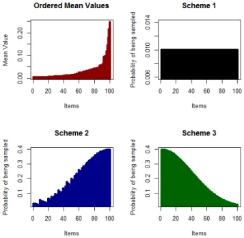
As mentioned, the entropy, or uncertainty, of a variable is derived from its initial probability of success. The probability of sampling based on entropy is a function of the x = [0, 2.5] segment
of a normal (Gaussian) distribution as reported in figure 3.3. The probability of a variable being sampled will therefore vary from a scale of 0.40 at the highest, to 0.0175 at the lowest. In other words, the odds of variables being sampled is about 23 times greater at the highest level compared to the lowest level (0.40/0.0175). Variables are assigned the probability of being sampled as a function of their rank: they are first ranked according to their entropy and they are attributed a probability of being sampled following this distribution. The distributions are the same for both conditions (2) and (3), but the ranking is reversed between the two of them. For the uniform condition (1), all variables have equal probability of being sampled.
Figure 3.3 Sampling probability distribution used for the schemes 2 and 3
We have conducted a simulation study of such sampling schemes. The details of the experi-mental conditions and the results are described below.
3.4.2 The Process
Our simulations consist in 100-fold cross-validation runs. In each run, different training and validating sets are built based on our three schemes described in previous subsection. The proportion of total missing values inserted in the training sets is half of the data. Testing datasets contain no missing values. We compare the performance of the models on the three different sampling schemes in terms of average number of Incorrectly Classified Items (ICI) and also the average Root Mean Square Error (RMSE).
To determine whether our results are statistically significant, for each model, 2-tailed paired t-tests are run on the pairs scheme2/scheme1 and scheme3/scheme1 on the results of 100 folds.
3.4.3 Datasets
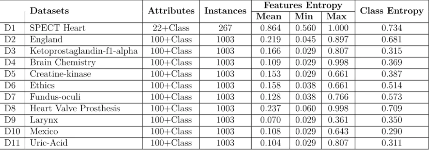
The experiments are conducted over 11 sets of real binary data. Table 3.1 reports general statistics on these datasets. The first dataset in the list, SPECT Heart, is from UCI Machine
Learning Repository (Bache and Lichman, 2013) and others are from KEEL-dataset Repos-itory (Alcalá et al., 2010).The numbers of instances in training and validating datasets are taken to be 90 and 10 percent of the instances in the datasets respectively.
Table 3.1Datasets - The Mean, Minimum and Maximum of the attribute entropies have been listed
Datasets Attributes Instances Features Entropy Class Entropy
Mean Min Max
D1 SPECT Heart 22+Class 267 0.864 0.560 1.000 0.734 D2 England 100+Class 1003 0.219 0.045 0.897 0.681 D3 Ketoprostaglandin-f1-alpha 100+Class 1003 0.166 0.029 0.807 0.315 D4 Brain Chemistry 100+Class 1003 0.109 0.029 0.998 0.369 D5 Creatine-kinase 100+Class 1003 0.153 0.029 0.661 0.387 D6 Ethics 100+Class 1003 0.158 0.038 0.661 0.514 D7 Fundus-oculi 100+Class 1003 0.128 0.038 0.766 0.573 D8 Heart Valve Prosthesis 100+Class 1003 0.237 0.060 0.998 0.709 D9 Larynx 100+Class 1003 0.070 0.029 0.361 0.350 D10 Mexico 100+Class 1003 0.108 0.029 0.643 0.290 D11 Uric-Acid 100+Class 1003 0.104 0.029 0.807 0.311
3.5 Results
Figure 3.4 illustrates the way we conduct the sampling taking the Ketoprostaglandin-f1-alpha Dataset as an example. The upper-left graph reports the initial probability of each of the 100 attributes, and the other three graph report the probability of sampling the variables. Table 3.2 reports the average percent of incorrectly classified items (ICI) for the methods based on the different sampling schemes. It also compares the performance of the methods based on average Root Mean Square Error (RMSE). As it is clear from the table, for this dataset, the performance of Naive Bayes improves under the sampling scheme 2. Logistic Regression performs better under scheme 3 and also, compared to other schemes, performance of TAN under scheme 3 is superior.
Results of conducting 2-tailed paired t-tests on the pairs scheme2/scheme1 and scheme3/scheme1 for the models on obtained results of 100 folds have been illustrated in tables 3.3 and 3.4. As the tables reflect, very small p-values show that there are very strong evidences against null hypothesis in those mentioned cases and therefore, our results, concluded from table 3.2, are statistically significant.
We have conducted similar simulations and evaluations for the other datasets. Our results show that Selective Sampling can effectively improve the performance of the classification
methods in most of the datasets. Table 3.5 reports the percent of datasets on which Selective Sampling schemes compared to uniform sampling, result in better classification performance. As it can be seen from the table, the performance of TAN in all of the datasets is improved by applying the third scheme of sampling.
Figure 3.4 Ketoprostaglandin-f1-alpha Dataset
Table 3.2 Performance comparison for the different techniques under the different schemes of sampling for Ketoprostaglandin-f1-alpha dataset (ICI-Incorrectly Classified Items and RMSE-Root-Means-Squared-Error)
Measure Scheme 1 Scheme 2 Scheme 3 NB Average Percent of ICI 4.37 3.84
*** 4.25
Average RMSE 0.20 0.18*** 0.19
LR Average Percent of ICI 6.12 14.73 5.05
**
Average RMSE 0.24 0.35 0.21**
TAN Average Percent of ICI 4.95 4.57 3.42
***
Average RMSE 0.20 0.18 0.16***
Table 3.3 Results of running a paired t-test on the obtained results of 100 folds based on average Pct. ICI
Pairs t Mean of the Differences p-value
NB Sch2/Sch1 -3.83 -0.524 0.000225 Sch3/Sch1 -1.25 -0.117 0.213 LR Sch2/Sch1 6.52 8.61 0 Sch3/Sch1 -3.31 -1.07 0.0013 TAN Sch2/Sch1 -1.49 -0.379 0.138 Sch3/Sch1 -7.92 -1.53 0 (df=99, Confidence Interval=95%)
Table 3.4 Results of running a paired t-test on the obtained results of 100 folds based on average RMSE
Pairs t Mean of the Differences p-value
NB Sch2/Sch1 -4.21 -0.0134 0.000056 Sch3/Sch1 -0.993 -0.00192 0.323 LR Sch2/Sch1 7.53 0.114 0 Sch3/Sch1 -3.1 -0.0228 0.00253 TAN Sch2/Sch1 -2.56 -0.0128 0.0119 Sch3/Sch1 -8.39 -0.0356 0 (df=99, Confidence Interval=95%)
Table 3.5 Percent of datasets on which Selective Sampling classification performance results are better (p<0.05) than Scheme 1
Scheme 2 Scheme 3 Total
NB 9.1% 45.5% 54.6%
LR 9.1% 45.5% 54.6%
TAN - 100% 100%
It should be mentioned that although, for example, in 54.6% of the datasets Selective Sam-pling improves the classification performance of Naive Bayes, it doesn’t imply that in the rest of the datasets (45.4%), Scheme 1 is the superior one; rather, as table 3.6 shows, only in 27% of the datasets uniform classification performance results are better (p<0.05) than just Scheme 2 and in none of the datasets it yields better results than Scheme 3.
Table 3.6 Percent of datasets on which Scheme 1 classification performance results are better (p<0.05) than Scheme 2, Scheme 3 or both of them
Sch.1 is better than Sch.2 Sch.3 Both
NB 27% 0 0
LR 81.8% 36% 27%
TAN 63.6% 0 0
3.6 Conclusion
These results confirm that based on a heuristic that relies on attribute entropy, Selective Sampling can improve the performance of the classification methods. Selective Sampling in all of the datasets improves the performance of TAN classifier. In more than half of the datasets (54.6%) it results in better prediction performance for both NB and LR classifiers. Results also show that lower sampling rate of missing values for high entropy variables (Scheme3) brings a higher predictive performance than for the high entropy or the uniform scheme. Further analysis and investigations are required to better explain these results. How should we explain the performance differences between the sampling schemes? What is the best sampling scheme in a given context? These are some interesting questions that are left open. Nevertheless, this investigation shows that we can influence the predictive performance of a classifier with partial data when we have the opportunity to select the missing values. It opens interesting questions and can prove valuable in some contexts of application.
CHAPTER 4 AN ADAPTIVE SAMPLING ALGORITHM TO IMPROVE THE PERFORMANCE OF CLASSIFICATION MODELS
This chapter1 extends the former study to assess the performance of the selective sampling
heuristics without assuming the prior information, a process we refer to as Adaptive Sampling and helps guide the sampling on the fly.
4.1 Chapter Overview
Given a fixed number of observations to train a model for a classification task, a Selective Sampling design helps decide how to allocate more, or fewer observations among the variables during the data gathering phase, such that some variables will have a greater ratio of missing values than others. In previous chapter, we established that conducting an informed selective sampling which relies on features’ entropy can improve the performance of some classification models. However, the results of the study were obtained given a priori information on the entropy of each variable. In realistic settings such information is generally not available. We now investigate whether the gains observed with a priori information hold when such information is not given.
The remainder of the chapter is organized as follows. We first define the term Adaptive Sampling in section 4.2 and then in section 4.3, explain our experimental methodology. In section 4.4, the results are presented and discussed. Finally, We wrap up the chapter with some concluding remarks.
4.2 Adaptive Sampling
Adaptive sampling is a technique that is enforced while a survey is being fielded—that is, the sampling design is modified in real time as data collection occurs—based on information gathered from previous sampling that has been completed. Therefore, when sampling or ’allocating’ adaptively, sampling decisions are dynamically made as data is gathered.
1This study has been published at the following venue: Ghorbani, S. and Desmarais, M.C. (2014) An
Adaptive Sampling Algorithm to Improve the Performance of Classification Models. In Proceedings of the 8th European Conference on Data Mining, pages 21-28. Lisbon, Portugal.
4.3 Methodology
Our experiments have been carried out using the same classifier models and the 11 datasets introduced earlier in Chapter 3. We have also used the three sampling schemes described in previous chapter (i.e., uniform, low entropy and high entropy sampling). The process and the details of the experimental conditions are explained below.
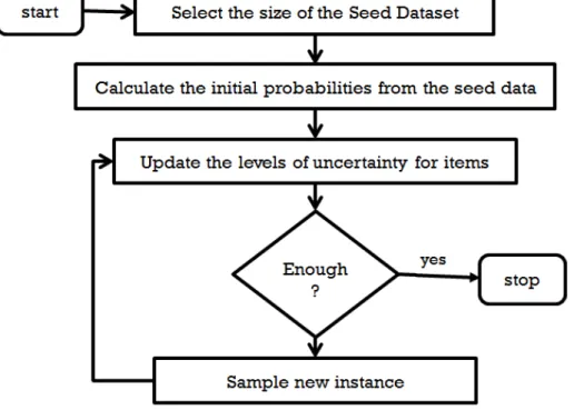
4.3.1 Adaptive Sampling and Seed Data
To conduct our sampling designs in an adaptive manner we start with a small seed dataset. Initial probabilities are obtained from the seed dataset and then entropy values are extracted. Then the algorithm samples feature observations based on the three different schemes. Levels of uncertainty (entropies) for all of the variables are updated based on what have been sampled so far. This process is repeated until the final sampling criterion, which in this study is to reach a fixed number of observations. Figure 4.1, shows a simple flowchart of the algorithm. In this study 3 different sizes for the seed dataset are: 2, 4 and 8 records.