Étude de l’hydrodynamique stellaire moyennant le code PLUTO

(1)

REPUBLIQUE ALGERIENNE DEMOCRATIQUE ET POPULAIRE Ministére de l’enseignement supérieur et de la recherche scientifique

Université El-Hadj Lakhdar - BATNA 1 Faculté des Sciences de la matiére

Département de Physique

T H É S E

Présentée par

Zoubida AHMANE

En vue de l’obtention du

Diplôme de Doctorat troisiéme cycle

Specialté : MATIÉRE-RAYONNEMENT et ASTROPHYSIQUE

Étude de l’hydrodynamique stellaire moyennant le code

PLUTO

Simulation des effets de photoionisation sur les jets YSO

Soutenue le 23 september 2020 Devant le jury

Président: Pr. Y. Delenda U. Batna 1 Rapporteurs: Pr. A. BOULDJDERI U. Batna 1

Pr. S. MASSAGLIA U. Torino, Italy Examinateurs: Pr. A. Sid U. Batna 1

(2)

Study of stellar hydrodynamics using

PLUTO code

PhD joint with

Hadj Lakhdar Batna 1 University

Studi di Torino University

Zoubida AHMANE

(3)

PhD joint with

Hadj Lakhdar Batna 1 University Studi di Torino University

T H E S I S

by

Zoubida AHMANE

to obtain the degree of

DOCTOR OF HADJ LAKHDAR BATNA1 UNIVERSITY Specialty : ASTROPHYSICS - PHYSICS and RADIATION

Study of stellar hydrodynamics using PLUTO code

Simulations of protostar-driven photoionization in Herbig-Haro Jets

Thesis defense on September 23 th 2020 with the following dissertation committee Pr. Y. Delenda Chairperson U. Batna1

Pr. A. BOULDJDERI Supervisor U. Batna1

Pr. S. MASSAGLIA co-Supervisor U. Torino, Italy

Pr. A. Sid Referee U. Batna1

(4)

Study of stellar hydrodynamics using PLUTO code Zoubida AHMANE

Copyrights 2020 Zoubida Ahmane

(5)

Abstract

Recent studies showed that observations of line emission from shocks in YSO jets require a sub- stantial amount of ionization of the pre-shock matter. Photoioniza-tion from X-ray emitted close to the central source may be responsible of the initial ionization fraction. The aim of our work is to study the effect of X ray photoioniza-tion, coming from the vicinities of the central star, on the ionization fraction inside the jet that can be advected at large distances. For this purpose we have performed axisymmetric MHD jet launching simulations including photoionization and opti cally thin losses using PLUTO. For typical X-ray luminosities in classical T.Tauri stars, we see that the photoionization is responsible for ionizing to 20%_{− 30% the} jet close to the star causing also its decolimation.

Keywords YSO- jets , X-rays; Résumé

Des études récentes ont montré que l’observation de raies d’émission issues des chocs dans les jets YSO exige un taux élevé d’ionisation de la matiére en amont du choc. La photoionisation due aux rayons x émis au voisinage de la source centrale pour-rait être responsable de la fraction d’ionisation initiale. Le but de notre travail est d’étudier l’effet de la photoionisation des rayons X issues des voisinages de l’étoile centrale, sur la fraction d’ionisation au sein du jet qui peut être advecté á de grandes distances. Pour cela, nous avons réalisé une simulation MHD du lancement d’un jet axisymétrique prenant en compte la photoionisation et les pertes optically thin en

(6)

utilisant le code PLUTO. Pour des luminosités X typiques dans les étoiles T Tauri classiques, nous voyons que la photoionisation est responsable de l’ionisation du jet á20%− 30% au voisinage de l’étoile causant aussi son décollimation.

(7)

List of Tables

(11)

List of Figures

1 The jet from the close M87 galaxy in X-ray, radio and optical bands. Image Credits: X-ray: NASA/CXC/MIT/H.Marshall et al. Radio:

F.Zhou, F.Owen(NRAO), J.Biretta(STScI) Optical: NASA/STScI/UMBC/E.Perlman et al. . . 21

2 Zoom on HH34 jets from down to 12 light year long jet. Upper left: This is a small part of the Orion Molecular Cloud Complex, a giant region of gas and dust undergoing active star formation some 1500 light-years away. The three HH objects labelled in green have been subjects of intense study by the NASA/ESA Hubble Space Telescope over several years, resulting in a better understanding of how the mate-rial ejected from stars interacts with the surrounding medium. Image Credit: Z. Levay (STScI), T.A. Rector (University of Alaska Anchor-age), and H. Schweiker (NOAO/AURA/NSF). Lower right: Image Credit: ESO Lower middle: Image Credit: ESA/Hubble NASA Lower left: Image Credit: Bo Reipurth (CASA/U. Colorado) et al., HST, NASA . . . 22 3 HH object 46/47. HH 46 is the nebula on lower left, while HH 47 is

in the upper right. HH 47B connects the two. Image Credit: Hubble Space Telescope. . . 23

(12)

4 HH30: The HH30 system is 450 light years away in the constellation of Taurus. HH34: The HH34 is 1500 light years far away in the vicinity of Orion nebulae. HH47: The HH47 is 1500 light years far away located at the edge of the Gum nebulae. Image Credit: Hubble Space Telescope. . . 24 1.1 This Hubble Space Telescope image shows the bright blobs at the end

of opposing jets due to shocks with ambient medium where the jet has been heated emanating from the star. Located near the Orion nebula, these nebulosities have catalog designations HH1 and HH2 for their discoverers astronomers George Herbig and Guillermo Haro. Image Credit: J. Hester (ASU), WFPC2 Team, NASA . . . 27 1.2 Stages of low mass star formation showing progression from

molecu-lar cloud towards the pre main sequence, with its respective Spectral Energy Distribution (SED) [Maury, 2009] [André, 2001]. SED plots adapted from figures [Lada, 1985] and [Tachihara et al., 2007] . . . . 30 1.3 Approximately 410 light-years away, Barnard 68 is one of the nearest

dark clouds. Image credit: European Southern Observatory (ESO). . 31 1.4 An infrared image of the IRAS 23011+6216 of the Cepheus E

em-bedded outflow, obtained by combining three publicly available IRAC band images. 8µm emission is presented as red, 4.5µm as green and 5.8µm as blue. The green nebulosity is believed to be from carbon monoxide molecules excited by outflows. The data was originally pub-lished by [Noriega-Crespo et al., 2005]. . . 33 1.5 HH7-11 jet water maser emission toward the region N GC1333 near

SV S13 observed at three different epochs over 50 days, a space veloc-ity of 13.6km/s is calculated at an inclination of 6 degrees from the plane of sky [Wootten et al., 2000]. . . 35

(13)

1.6 From left to right : Class 0 jet source HH212 in H22.12µm [Zinnecker, 2002], Class I HH111 archetypal example of a outflow from a Class I protostar observed in H22.12µm ( turquoise) and in [S II] and Hα

[Reipurth et al., 1997], archetypal example of a atomic outflow from a Class II micro jet DG Tau(image taken from [Cabrit, 2002]) observed in [Fe II] (in red and color ) surrounded by a molecular component H2(yellow) [Agra-Amboage et al., 2011] . . . 38

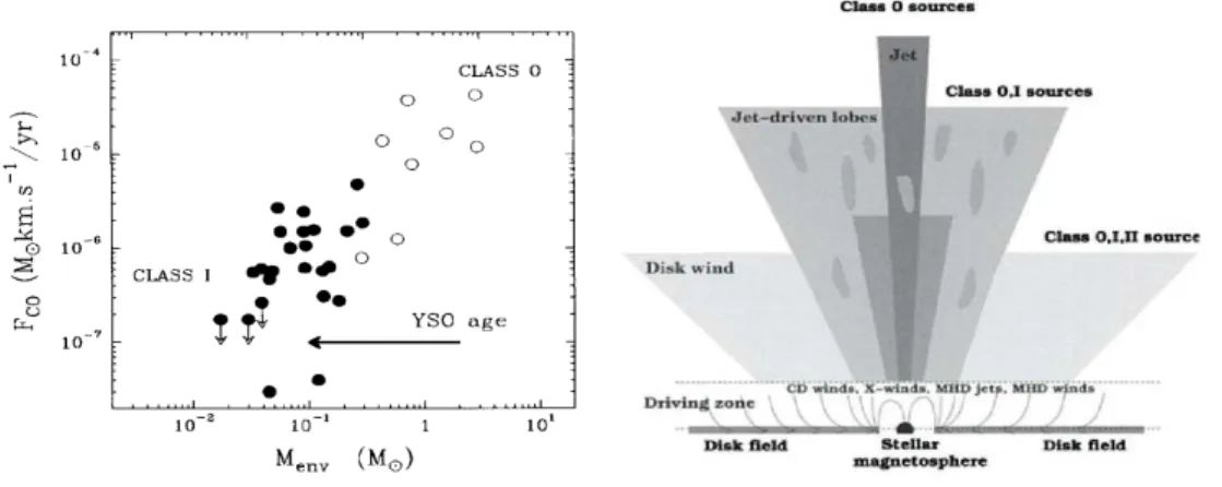
1.7 Left panel represents the outflow proprieties as function of proto-stellar age. The right panel is cartoon illustration of the measure-ments done in the left panel showing the classification picture of the outflow strength as to be inversely proportional to envelope which gets accreted over time [Schulz, 2007a] . . . 39 1.8 Simulation performed with ZEUS hydrodynamic code representing the

front section, 2.5D axisymmetric adiabatic jet simulation with the characteristic jet features labelled. The map depicts a logarithmic scale of density in units ofg/cm3_{, the brighter shading is higher density}

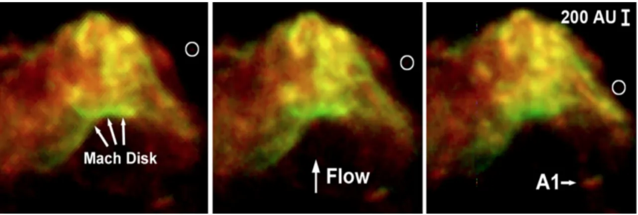
and darker shading is lower density. The jet beam is traveling along a stationary uniform ambient medium [Moraghan et al., 2006]. . . . 41 1.9 Bow shock and Mach disk at the head of HH 47A outflow. The bow

shock travels from the bottom to the top in all panels, which have been registered to align the Mach disk near the center. The circled object is the driving source. The Mach disk is clearly defined as a linear Hα in green, emission feature located at the base of the bow

shock [Heathcote et al., 1996]. The area between the bow shock and the Mach disk is clumpy and radiates in both Hα and [SII] in red;

for the three epochs. This figure is taken from a paper by [Hartigan et al., 2011]. . . 42

(14)

1.10 Straight morphology of knots aligned along the jet (e.g.Top:HH34 outflow). This figure is taken from paper by [Hartigan et al., 2011]. Middle: HH111 observed by HST. Image Credit: ESA Hubble ma-terial prior to 2009. Misaligned wiggles morphology (e.g Bottom: HH110 figure taken from [López et al., 2010]) The individual HH objects that make up the flow are labelled A to J. . . 44 1.11 Structure of an oblique C shock with ambipolar diffusion MA = 5

(left panel),MA = 10 (right panel) and θ = π/4. The displayed shock

values are (ρ = 1 vx = 4.45, 9.47 vy = 0 Bx = √1₂ By = √1₂ p = 0.01).

Profiles of neutral density (magenta) and ion (cyan) velocity compo-nents obtained from the equation of relative drift velocity between ion and neutrals,vi = v +_γ 1

adρiρ(∇×B)×B and magnetic field components. 46

1.12 Time evolution of p< B2

z > , the root mean square of the magnetic

field in the z direction for γad = 1000 (top) , 500 (middle) and 100

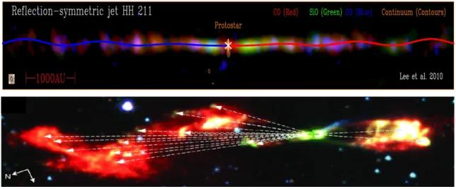
(bottom) in the test of Alfven waves with ambipolar diffusion. . . 48 1.13 Top: C shape, the HH211 Class 0 molecular jet imaged with the SMA

at0.3” _{resolution. The CO, SiO, SO, and 0.85 mm continuum are red,}

green, blue, and orange (contours), respectively. The jet is clearly seen on both sides of the source with more than one cycle of wiggle. The wiggle is reflection-symmetric about the source and can be reasonably fitted by an orbiting source jet model [Lee et al., 2010]. Bottom: S shape, three color spitzer IRAC image of the L1157 outflow blue 3.6 µm, green 4.5µm and red 8.0µm image taken from [Frank et al., 2014] 50 1.14 Comparison of observed line ratios (symbols) in DG Tau microjet

panel (a)(b) and jets +HH object panel (c)(d) with the theoretical predictions of line ratios as predicted from radiative shock model [Har-tigan et al., 1994] (green curve). Turbulent mixing layers [Binette et al., 2000] (dashed curves), and ambipolar diffusion (solid line) [Gar-cia et al., 2000]. Taken from [Cabrit, 2002] . . . 52

(15)

1.15 Log10 scale plot on the jet axis of line ratio with X-ray pre ionisation included (lines) in comparison with the observed line ratios (symbols) for the three doublets of [S II] 6716+6731 Å, [O I] 6300+6363 Å, and [N II] 6548+6583 Å [Teşileanu et al., 2012]. . . 53 2.1 Global view of magnetised accretion ejection structure (MAES) around

young star [Zanni and Ferreira, 2013]. Logarithmic density is displayed in color. Dashed lines represent Alfven surfaceSA(whereVp = Bp/4πρ

). The blue arrows represent the poloidal speed. The magnetic field lines are traced in white. The yellow curves illustrate the three differ-ent compondiffer-ents of jet launching namely: disk-wind, stellar-wind and magnetospheric-wind. . . 57

(16)

2.2 Top: Classes of stationary winds. (a) "disk winds", when the mag-netic flux threading the disk is large enough and extended radially so that the whole accretion disk drives jets (r > 0.1AU ). The Alfven sur-face SA is expected to adopt a conical shape. (b) "X-winds", when

the magnetic flux is small and only a tiny region near co-rotation is driving jets. The Alfven surface SA can be either convex or

con-cave. (c) Stationary stellar winds pressure driven through an open field lines anchored onto slowly rotating star, the Alfven surface SA

is schematically drawn. Bottom: Three simple unsteady winds from axisymmetric star-disk magnetospheric interactions: (d) "Y- type" in-teraction obtained when the stellar magnetic moment is anti-parallel to the disk magnetic field. (e) "X-type" configuration obtained when the stellar magnetic moment is parallel to the disc magnetic field. A magnetic X-point is generated at the disk midplane where the two fields cancel each other. Unsteady wind can be launched above this reconnection site. (f ) CME like ejection produced due to differential rotation between the star and the disk leading to violent reconnec-tion, such event may occurs with any anti parallel magnetospheric interaction. Adapted from [Ferreira et al., 2006] . . . 60 2.3 A schematic view of jets through seven order of magnitude in scale

starting from the launching mechanism to the physics of feedback on cluster and clouds [Frank et al., 2014] . . . 61 2.4 Correlation between the ejection rate and accretion rate of T Tauri star

from the optical observation [Hartigan et al., 1995] in black [Gullbring et al., 1998] in orange, as well as for optical jets from Class I. The dashed curve represent M˙ej/ ˙Macc = 0.1, figure adapted from [Cabrit,

(17)

2.5 HST Hα image of the HH 30 jet-disk system taken from [Ray et al.,

1996]. The jet is seen to be perpendicular to the circumstellar disk, which is indicated by the vertical dark flared disk illuminated from the inside by the central, obscured star. . . 64 2.6 Width of the jet versus the distance from the source in AU . From

jet of Class II sources in black and jet from Class 0 red [Cabrit, 2007] showing that outflow from embedded source Class 0 is collimated on similar scale. . . 65 2.7 Position-velocity contour diagrams in selected emission lines observed

in the optical regime. Note that the [O I] emission traces both the higher and lower velocity jet material. [Coffey et al., 2007] this trans-verse velocity decrease Vr in DG Tau well produced by extended disk

wind with Rout ≈ 3AU [Pesenti et al., 2004]. Note the increase in jet

collimation with increasing velocity. . . 66 2.8 Class II: HH30 in CO, class II [Louvet et al., 2016], ALMA ,Class

I: CB 26 in CO with PdBI [Launhardt et al., 2009]. Class: massive source I SiO maser VLBA [Maury, 2009] [Vaidya and Goddi, 2012] . 67 2.9 Chandra Xray view of Orion nebula is the nearest rich stellar nursery,

located just 1,500 light years away. Analysis of the COUP X-ray image revealed 1616 individual X-ray sources, 1400 of which can be identified with young stars in the cluster. Image Credit: E.Feigelson K.Getman (PSU) et al., CXO, NASA. . . 68 2.10 X-ray jet From30 AU to parsec scales DG Tau 30 AU [Güdel et al.,

2008] [Güdel et al., 2007] , DG Tau1200 AU , HH80 2.5 pc [Pravdo et al., 2004] . . . 69 2.11 Physical quantities along theHH30 using "BE" technique (a) is [SII]

emission, (b) ionisation fraction, (c) electron temperature, (d) total density, (e) filling factor, and (f) mass flux [Ray, 2007]. . . 73

(18)

2.12 Outflow envelope interaction: widening of outflow cavity over time from left to right respectively Class 0 [Tobin et al., 2013],Class I [Arce and Sargent, 2006] and Class II [Lee et al., 2007]. . . 75 2.13 Our changing view of the size of the giant molecular outflow from

the Class I as ejected from the star B5-IRS1 presented as orange star symbol located at the image center. The dotted square presents the original extent from [Bally and Talay, 1996]. The dashed square shows the region shown by [Yu et al., 1999]. The dark blue/red contours show the map from the cloud-scale CO outflow survey of [Arce et al., 2010]. Image taken from [Frank et al., 2014]. . . 76 2.14 Parsec jet observed inHαand[SII] we see ejection from recent epochs

as we go farther distances and as we move out we get earlier ejection. The jets fragments on shocks and bows highlighted by yellow circle forming S shape which come from precession [Frank et al., 2014]. . . 77 3.1 Left panel: two magnetic surfaces ψ1 and ψ2 separated by δr. Right

panel: represents poloidal magnetic field line. The poloidal velocity and magnetic field are parallel Bp||vp, whereas the electric field and

the flux function are normal [Romero.G.E., 2014]. . . 82 3.2 Solution of momentum equation of stellar wind [Lamberts-Marcade,

2012] . . . 91 3.3 The Weber Davis magnetised and rotating wind [Tsinganos, 2007] . . 92 3.4 (a): Solutions topology passing through the critical points are denoted

as ua1, ua2 with zero pressure at infinity and ub2, ub2 with non-zero pressure. The first two critical points are (S,A) slow magnetosonic and Alfven while the fast point is shown in (b). (b): Closeup of (a). The third singularity fast magnetosonic can also be distinguished near to the Alfven point. Image credit: [Weber and Davis Jr, 1967]. . . 94 3.5 Ulysses data on solar wind speed. From [Sauty et al., 2005] . . . 95

(19)

3.6 The regions of magnetically accelerated Disk wind. From the disk surrounding medium up to Alfven surface the magnetic field domi-nates over gas pressure and kinetic this region is called centrifugal acceleration. Left inset: presentation of a gas particle like a "bead on a wire" attached to the poloidal magnetic field line. Right inset: beyond the Alfven distance the field lines lag behind the rotation of their footpoints and are coiled into a spiral [Spruit, 2010]. . . 98 3.7 Selfsimilar field line sturctures (a) radial self similarity where the ratio

ω1/ω2 for the intersection of any poloidal line with a cone is the same

of any value of θ; (b) meridional self similarity, where the ratio at (a) is the same for any spherical surface r = const [Tsinganos, 2007] . . . 100 4.1 Effective cooling curve in temperature range from103 _to₁₀6 _{K curve}

in(magenta) . Ionisation fraction at equilibrium for Hydrogen curve in(green). The result is obtained using SNEq module in PLUTO code. 106 4.2 Zoom picture of AMR map at the vicinity of the star region, the coarse

level is lmin = 0 (red), the highest resolution is lmax = 4 (magenta). The corresponding refinement map shows that refinement happens at the star vicinity around 8 AU. Very high resolution is limited to a small region close to the accretion disk at the boundary. . . 111 4.3 Scheme of integration of optical depth from origin to cell center. . . 112 4.4 (a)(b) Zero gradient condition right picture and (c)(d) force free

con-dition left picture, highlighting the effect of spurious collimation due to artificial Lorentz force coming from right most boundary. . . 118 4.5 Jet integrals along the magnetic field line rooted in the innermost

disk. The jet specific angular momentumΩ, the mass load k, the field angular velocity L, the jet specific energy E, and the specific entropy Q. . . 119

(20)

4.6 Jet specific energy contributions along the vertical direction z. Dif-ferent energy components are indicated by colors: kinetic (green), magnetic (red), gravitational (magenta), and thermal (black) energy. 121 4.7 Mass loss rate as a function of time at different heights (yellow) along

the disk, (magenta) at1000AU and (blue) at 2000AU. The figure show decrease in the ejection as we go further from the disk surface. . . 123 4.8 From top to bottom, we show four snapshots of the temporal evolution

corresponding to t = 25, 100, 175 and 250 yrs. In the first panel (A) shows the logarithmic maps of the temperature ( in units of 104 _K)

for the adiabatic case. The second three panels (B, C, D) compares the temperature maps when cooling is included (upper half) and the adiabatic case (lower half). The jet propagates from left to right. . . 125 4.9 Top panel: velocity along the z direction in km/s profile - adiabatic

and cooling cases, - at different heights. Bottom panel: temperature profile (in K) - adiabatic and cooling cases, - at different heights, corresponding to t = 175 yrs. . . 126 4.10 Top panel: From top to bottom, we show two snapshots of the

loga-rithmic ratio of the absolute value of the toroidal magnetic field over the poloidal, the temporal evolution corresponding to t = 125 and 250 yrs. The solid lines in (red, black and green) indicate the criti-cal surfaces i.e. Alfvénic, fast magnetosonic and slow magnetosonic respectively. Bottom panel: Zoomed image of the jet base, with log-arithmic coordinate along z indicating the critical surfaces; the solid lines in (red, black and green) corresponds to Alfvénic, fast magne-tosonic and slow magnemagne-tosonic respectively. The jet propagates from left to right. . . 127 4.11 SNEq (Simplified Non Equilibrium Cooling):Ionization fraction of the

jet material when only cooling is included (no heating). Snapshots are shown at t = 100, 150 and t = 250 yrs. . . 128

(21)

4.12 (SNEq+Heating) Bottom panel: Maps of the total ionization fraction of the jet material for different luminosity L = 1028 _erg/s, _{L = 10}32

erg/s at different times t = 100, 150 and t = 250 yrs. Top panel: The corresponding zoomed image of total hydrogen ionization fraction at time t = 100 yrs. . . 129 4.13 Ionisation fraction profiles for different luminosity L = 1028 _erg/s,

L = 1032 _{erg/s at different heights, corresponding to}_{t = 250 yrs.} _{. . 130}

4.14 Left panel: Zoomed logarithmic 2D map of the coolingΛcinerg cm−3 s−1.

Right panel: Zoomed image of the logarithmic 2D heating map _{H in} erg cm−3 _s−1_{, for luminosity} _{L = 10}32_{erg/s and L = 10}28_{erg/s, at}

(22)

Preface

Outflows from astrophysical objects have been observed in several astrophysical sys-tems. The first astrophysical outflow "Jets" was observed by Heber Curtis in lick observatory on 1917 a thin line of matter connected to the elliptical galaxy M87 Figure (1.3).

Much later, jets were observed inside our galaxy: protostellar jets around young forming stars (0.3 _{− 3M}) [Hartigan et al., 1995] (e.g. HH30 figure (1.2), HH34

figure (2),HH47 figure (1.1)) and some X-ray binaries (e.g. SS433, GRO J 1655-40, GRO J0422+32), planetary nebula (e.g. the Egg Nebula, etc), symbiotic stars (e.g. R Aquarii, CH Cygni, etc), Cataclysmic variables (T Pycisdis, etc) to black holes at the center of AGN (e.g. M87, 3C273, NGC4261, etc), as massive as(5_×108_M

) [Ray,

2007]. Because of the similarities based on their morphology, same physical mecha-nism is believed to be at work at all scales.

(23)

Figure 1: The jet from the close M87 galaxy in X-ray, radio and optical bands. Image Credits: X-ray: NASA/CXC/MIT/H.Marshall et al. Radio: F.Zhou, F.Owen(NRAO), J.Biretta(STScI) Optical: NASA/STScI/UMBC/E.Perlman et al.

The relatively small distance to protostellar jet; made them a good candidates for comparing and discriminate between theoretical models of jets formation and propagations.

A protostellar jet is a highly supersonic magnetised outflow which heralds the birth of star while it is still embedded, out of sight in the molecular outflow. In partic-ular, Herbig Haro (H-H) objects like HH30, DG tau, RW Aur, [Bacciotti et al., 1999] [Lavalley et al., 1997]; [Lavalley-Fouquet et al., 2000] [Bacciotti et al., 2002], [Mel-nikov et al., 2009]are detected in stellar forming regions. T-Tauri stars characterised by highly collimated ejection, associated with an emission being identified as due to shocks from the gas that has been heated and compressed [Schwartz, 1975]; [Do-pita, 1978] emanating directly from the protostars [Mundt et al., 1985]; [Lada, 1985] , [Maurri et al., 2014].

(24)

Figure 2: Zoom on HH34 jets from down to 12 light year long jet. Upper left: This is a small part of the Orion Molecular Cloud Complex, a giant region of gas and dust undergoing active star formation some 1500 light-years away. The three HH objects labelled in green have been subjects of intense study by the NASA/ESA Hubble Space Telescope over several years, resulting in a better understanding of how the material ejected from stars interacts with the surrounding medium. Image Credit: Z. Levay (STScI), T.A. Rector (University of Alaska Anchorage), and H. Schweiker (NOAO/AURA/NSF). Lower right: Image Credit: ESO Lower middle: Image Credit: ESA/Hubble NASA Lower left: Image Credit: Bo Reipurth (CASA/U.

(25)

Figure 3: HH object 46/47. HH 46 is the nebula on lower left, while HH 47 is in the upper right. HH 47B connects the two. Image Credit: Hubble Space Telescope.

(26)

Figure 4: HH30: The HH30 system is 450 light years away in the constellation of Taurus. HH34: The HH34 is 1500 light years far away in the vicinity of Orion nebulae. HH47: The HH47 is 1500 light years far away located at the edge of the Gum nebulae. Image Credit: Hubble Space Telescope.

The treatment of this highly magnetised supersonic outflow in the presence of non ideal effects such as non equilibrium cooling radiation is twofold, firstly the need of examination of the effect of these latter on the energy and dynamics of the flow. Sec-ondly the inclusion of those effects helps as a good diagnostic for our flow. For those reasons an extensive effort is being put into modelling radiative cooling in simulation.

Teşileanu [Teşileanu et al., 2012] have found that10_{−20% of ionisation fraction, is} necessary to obtain a closer agreement between observed brightness distribution and simulated one. The purpose of thesis to emphasize on testing this basic hypothesis by considering the launching and large scale regions simultaneously which is further challenge, because of large scale dynamical range simulation and observation. Our

(27)

work is based on high spatial simulation that implies a large number of dynamical grid points.

In chapter 1 we set some basic notions regarding astrophysical jets and the envi-ronment in which they are encountered. We examine where the scenario of outflows comes from during star formation, their morphology, jet emission and jet physics be-fore going on to examine the observational properties and theoretical understanding of young stellar objects (YSOs) and their outflows.

In chapter 2 we describe the observed jet proprieties from origin to parsec scale: starting from star-disk scale, envelope and parent clump to cluster and molecular clouds scale.

In chapter 3 we highlight different theoretical model of outflows: disk-wind and stellar-wind model.

In chapter 4 we provide the necessary ingredients needed to model our jet launch-ing with the inclusion of non ideal effect ie: non radiative coollaunch-ing and photoionisa-tion, we describe in details the numerical methods used to carry out the simulation. We present our results and discussion, with analysis that can be made from this data.

Finally, in the last chapter 5 we give a brief conclusion of this work, its impli-cation in wider context and the different proposed axes that may be taken in future research.

(28)

Chapter 1 Introduction

The history of astronomy is a history of receding horizons

Edwin Powell Hubble

I

Protostellar Outflows and Herbig-Haro Objects

The presence of outflow from young stars was discovered by George Herbig and Guillermo Haro who independently found that T Tauri stars could excite in the Burnham’s an emission nebula lines such as [S II] [O II] [Herbig, 1950] [Haro, 1952]. Prior to their discovery, it was already evident that YSOs had outflows. The puz-zling nebulous emission of Herbig Haro, named after them (HH objects hereafter) was identified as due to shocks cooling rather than photoionisation [Schwartz, 1975] [Do-pita, 1978]. Their spectra were dominated by low excitation species with line widths suggesting velocities up to several hundred km/s. Earlier [Osterbrock, 1958] spec-ulated that high velocity matter was some how responsible for the emission. The exact way of how these objects are linked to star formation was a mystery until another piece of puzzle appeared on scene, highly collimated outflows named "jets" were discovered emerging directly from the protostars [Mundt, 1986] [Reipurth et al.,

(29)

]. In the 80s with use of CCD cameras, their true nature, that combine these HH objects to the young stellar objects become clear. They are the termination shocks enhanced by jet outflow from nearby protostars [Mundt et al., 1985] [Lada, 1985]. Figure (1.1) presents an archytypical example of Herbig Haro object HH1, HH2 mov-ing in opposite direction with two bright blobs due to shocks with the interstellar medium [Herbig and Jones, 1981]. The discovery of other jets comes in picture eg (HH111) with usually similar basic structure, showing a chain of knotty structure or shocks along the jet emanating from a nearby young stellar object [Heathcote and Reipurth, 1992] [Hartigan et al., 2001].

Figure 1.1: This Hubble Space Telescope image shows the bright blobs at the end of opposing jets due to shocks with ambient medium where the jet has been heated emanating from the star. Located near the Orion nebula, these nebulosities have catalog designations HH1 and HH2 for their discoverers astronomers George Herbig and Guillermo Haro. Image Credit: J. Hester (ASU), WFPC2 Team, NASA

In the following, before we enter the heart of our work and describe the jets, we will first describe the protostar formation, since the ejection is produced during

(30)

the evolution process. We examine where the scenario of outflows comes in the big picture, before going on to examine the observational properties and theoretical understanding of young stellar objects (YSOs) and their outflows.

II

Jets in the Context of Star Formation

Protostellar jets and outflows are intrinsically linked to the star formation. Their presence is an essential ingredient of star evolution. Indeed, I) for all stars from Class 0, Class I and Class II, show that the mechanism of outflow is universal and very efficient; about10% of accreted matter is in the jet [Cabrit, 2007]. II) The core mass function is far too low from the initial mass function(IMF here after) in many em-bedded sources suggesting core to star efficiency of only30% [o Garatti et al., 2012]. III) The need of efficiently is for removing angular momentum from young stars and the surrounding disk to regulate the excessive spin up [Bouvier et al., 2007]. Thus, in this section we will review the processes involved during the low mass star formation to understand the interaction of protostellar jets with its central core. With the goal of identifying the conditions that lead to protostellar jets and outflows, with an emphasis onto the jet physical conditions across each phase [Frank et al., 2014], an excellent historical review can be found in [Ray, 2007] and [Schulz, 2007b].

Figure (1.2) shows the typical spectral energy distribution (SED hereinafter)

1 _{with the corresponding Bolometric temperature,} _T

bol, 2 and models of emission

regions through the star formation namely prestellar phase, protostellar phase and

1_{SED is a stringent tool to know the phase of star formation. Defined as the radiated power}

over a wavelength range,λ_{× S}λ, the infrared wavelength range (2 - 20µm) in this case.

2_{Bolometric temperature defined by [Chen et al., 1995] as the temperature of a blackbody having}

the same mean frequency as the observed continuum spectrum and where the "mean frequency" is the ratio of the first and zeroth order moments of the source spectra. It can be quantified by the following equation, where< ν >is the mean frequency of the observed spectrum [Smith, 2004] Tbol= 1.25_100GHz<ν> .

(31)

II. Jets in the Context of Star Formation

pre main sequence phase highlighting the four Class stages namely Class 0, Class I, Class II and Class III with an illustration showing how the system evolves at each stage.

II.1

Prestellar phase

A prestellar phase is defined as phase in which a gravitationnally bound core has formed in molecular cloud (MC hereinafter). Star formation takes place within MCs and as their name suggests, they are made of molecules, mainlyH2while other species

can be found in smaller quantities. They emit almost all of their radiation in the far infrared bend and at longer wavelengths indicating that the emitting matter must be very cold. The temperature in these clouds are 10 to 50 K typically, due to the heating and cooling mechanism. The former one is provided by cosmic rays and the emission from nearby stars. The latter is provided by absorption and collision of dust and gas particles present in the cloud leading to infrared energy. MC can be divided up into two types: Small molecular clouds or giant (SMC,GMC). The smallest star forming clouds popularly referred to as "Bok globules" [Bok and Reilly, 1947] are shown (1.3). Bok globules have typical masses of the order of0.1_{− 50M} diameters

of few tenths of parsec and average temperature about 10K [Nelson and Langer, 1999]. Giant molecular clouds (GMC) have masses of order of106_M

and diameters

up to250pc and higher ambient temperature 50_{−100K. MC are transient structures} and do not survive without radical changes for more than few times107_{years. There}

are also indications of the presence of magnetic fields with strength of few µG to a fewmG [Bourke et al., 2001].

(32)

Figure 1.2: Stages of low mass star formation showing progression from molecular cloud towards the pre main sequence, with its respective Spectral Energy Distribution (SED) [Maury, 2009] [André, 2001]. SED plots adapted from figures [Lada, 1985] and [Tachihara et al., 2007]

(33)

Figure 1.3: Approximately 410 light-years away, Barnard 68 is one of the nearest dark clouds. Image credit: European Southern Observatory (ESO).

It has been shown that supersonic turbulence [Larson, 1981] is a fundamental ingredient determining the MC morphology and dynamics; this turbulence is highly supersonic, with Mach numbers M = 5− 20 [Zuckerman and Palmer, 1974]. Hy-personic velocity fluctuations in the roughly isothermal molecular gas produce large density enhancement at shocks and can push the MC into a thermally unstable regime in which the gas can cools rapidly into a cold dense regime [Hennebelle and Pérault, 1999]. In addition, magnetic fields help to overcome the gravitational pull and stabilise cores against collapse [Shu et al., 1987] [Nakano, 1998]. We will see later on that the magnetic field not only supports the cloud from collapsing but it can also be a key ingredient for the jet launching. This equipartition of energies is indicative of the general stability and longevity of the clouds.

Nonetheless, since the ionisation level of the MC is particularly low; slippage between neutrals and ions occurs leading to ambipolar diffusion process. Thus the

(34)

ions leak out leaving the neutrals without magnetic support. The collapse occurs locally and can sweep up the gas into thin flocculent layers leading to local density enhancements, presenting filaments and clump-like structures and leading to its frag-mentation by large scale gravitational instability in the spiral arms [Stark and Lee, 2005] or by more scattered turbulent compression event driven by supernovae explo-sion [Vazquez-Semadeni et al., 1995] or magnetorotational instabilities MRI [Balbus and Hawley, 1998].

The end of this fragmentation process is pre stellar core (nH >= 105cm−3, D >=

0.05pc) [Bergin and Tafalla, 2007], often modelled as thermally supported Bonnor Ebert sphere. These cores take 3.0× 105 _{years to form a protostar [Kirk et al.,}

2007]T The mass distribution of dense core is that of IMF [Motte and André, 2001], t = 0 in figure (1.2) marked the formation of prestellar core i.e.: the initial region of MC that starts to collapse.

II.2

Protostellar phase

The process of gravitational collapse is part of the sequence of star formation that starts from giant molecular clouds that fragments into dense cores and then collapses. As the material collapses, the central regions become denser at the center than at the edges of the clouds and more centrally peaked. The collapse generates heat due to compression of the gas, with the cooling due to hydrogen molecules and dust. As the central regions become denser and reachs10−13_g _cm−3_{, an opaque hydrostatic}

object, the first core, is formed (Mass 10−2_M

,Radius 5.0AU , Temperature 1000K)

[Larson, 1969].

This first core continues to collapse until the temperature reaches 2000K, the molecular hydrogen dissociates through endothermic process. As a result of this contraction a core of 0.01M is produced, this phase is usually referred as "zero

age" of a star. It is also in this phase that the protostar becomes first visible in the infrared [Maury, 2009].

(35)

II.2.1 Class 0

Historically, the outflow powered by several Class 0 were discovered before the identi-fication of the central object. The first observation of Class 0 was proposed by [Andre et al., 1993] when observations at the submillimeter telescope have become possible. Class 0 objects are distinguished from other YSOs by large amount of dust surround-ing them, thus they became detectable at submillimeter wavelengths only since the radiation from the central source is absorbed by the surrounding dust. Today, some of the brighter Class 0 objects can be detected in infrared by the Spitzer Space Tele-scope, such as the Class 0 object IRAS 23011+6126 detectable at 3.5µm [Noriega-Crespo et al., 2005] (see Figure 1.4).

Figure 1.4: An infrared image of the IRAS 23011+6216 of the Cepheus E embedded outflow, obtained by combining three publicly available IRAC band images. 8µm emission is presented as red,4.5µm as green and 5.8µm as blue. The green nebulosity is believed to be from carbon monoxide molecules excited by outflows. The data was originally published by [Noriega-Crespo et al., 2005].

(36)

In this phase the process of accretion has become established enough that the accretion disk starts to form, most of the system’s mass is still actually in the disk gas, and the central core(Menv > Mstar + Mdisk) is still cold with a temperature

less than 70K. The SED of these objects is that of a cold black body, observable at submillimeter wavelengths. Despite their extremely low luminosity, the presence of Class 0 objects is revealed by powerful bipolar outflows and dense molecular jets emanating from their vicinity. The protostars of Class 0 accrete matter efficiently with an accretion rate of order ofMaccr105M/years [Bontemps et al., 1996].

Jet in Class 0

Molecular jets ejected at velocity ofv = 50km/s from the youngest protostars Class 0 are detectable in submillimetric and infrared ranges. As these Class 0 sources are embedded in envelope of gas and dust none of these jets are detectable in the optical range. Molecular jets detected in CO and SiO [Cabrit, 2007] have been detected at distances extending to 0.05− 0.1 pc scale. They have a knotty structure with a typical knots spacing 1000AU [Gueth and Guilloteau, 1999]; [Chandler and Richer, 2001]. An atomic component associated with these jets has been detected in [S I] [Fe II] and [Si II], via mid IR lines by the Spitzer telescope [Dionatos et al., 2009, Dionatos et al., 2010], characterised by moderate ionisation fraction of> 10−3_.

Certain sources, present show H2O jet, probing very strong shocks with a highly

bipolar structure [Furuya et al., 2002]. Figure (1.5) shows the discovery of water maser emission, observed with VLBA, associated with the source HH7-11 toward the regionN GC1333 near SV S13 with "molecular bullets" more typically from Class 0 jet [Wootten et al., 2000]. Figure(1.6) shows a very young molecular jet, archetypal example of a molecular outflow in Class 0 source HH212, located near the young IC348 stellar cluster in the Perseus molecular cloud at a distance of 300pc.

(37)

Figure 1.5: HH7-11 jet water maser emission toward the region N GC1333 near SV S13 observed at three different epochs over 50 days, a space velocity of 13.6km/s is calculated at an inclination of 6 degrees from the plane of sky [Wootten et al., 2000].

II.2.2 Class I

A Class I object, represents a more evolved object. As protostar’s surrounding envelope continues to collapse, the disk assumes a more flattened shape, so that more of the matter is contained in the protostar than in the surrounding disk and the ambient gas. Accretion and outflows continue to remove excess spin angular momentum from the system.

This Class I of objects have bolometric luminosity between 100K < Tbol < 700K.

From figure(1.2) we see that the black body curve has shifted to shorter wavelengths, and an additional infrared, due to the heating of surrounding heavy dust appears, the prominent absorption peak is believed to be due to silicate dust absorption at 10µm [Smith, 2004]. The Class I can last about 2× 105_years.

(38)

Jet in Class I

Jets from Class I sources are less intense than the ones from Class 0. In contrast to Class 0 jet, old molecular jets CO and Si are undetectable in this Class. However,H2

component associated with atomic jet is seen with Intermediate Velocity Component IVC 10_{− 50km/s at 1000 − 2000K [Davis et al., 2001]and [Herczeg et al., 2011].} Figure (1.6) shows an archetypal example of a outflow from a Class I protostar HH111 observed in H2. The extend jets are visible in optical range [O I] (6300 Å),

[S II] (6731 Å) or [Fe II](1.64µm) with shock velocity of 20−150km/s for jet velocity of 100_{− 400km/s.}

II.3

Pre-main sequence phase

Once the accretion starts to slow down and eventually stops the protostar is revealed as a pre main sequence star. The core reaches its final mass and becomes visible and continues its evolution in Hayashi track to become a main sequence star.

II.3.1 Class II

The Class II phase differs from the Class I one by the fact that the stellar wind has by now blown off most of the surrounding gas (except for the accretion disk), and by the temperature, has reached thousands of Kelvin. The bolometric temperature range for this class between 700K < Tbol < 3000K. The disk still has a slight infrared excess

on the back of stellar black body spectrum (see figure(1.2)); an ultraviolet excess may be visible the material is accreting onto the now exposed stellar surface [Smith, 2004]. These objects are also known as Classical T Tauri stars [Joy, 1945], named after the first discovered object of this type. The estimated age at this stage is 105_years.

(39)

Jet in Class II

Class II object have "micro jets" characterised by high velocity and well collimated, seen in optical lines [OI ],[SII ] and [FeII] out to distances of 1000AU [Dougados et al., 2000] probing faster shocks _{≥ 100km/s [Bacciotti et al., 2011]. The} molecu-lar components are almost undetectable, some of T Tauri represents molecumolecu-lar jets surrounding the atomic like DG Tau [Agra-Amboage et al., 2011], (see figure (1.6)). As the protostar evolves from Class 0 to Class II the molecular component becomes less intense and wider.

(40)

Figure 1.6: From left to right : Class 0 jet source HH212 in H2 2.12µm [Zinnecker, 2002], Class I HH111 archetypal example of a outflow from a Class I protostar observed in H22.12µm ( turquoise) and in [S II] and Hα [Reipurth et al., 1997],

archetypal example of a atomic outflow from a Class II micro jet DG Tau(image taken from [Cabrit, 2002]) observed in [Fe II] (in red and color ) surrounded by a molecular componentH2(yellow) [Agra-Amboage et al., 2011]

II.3.2 Class III

Class III represents the most advanced stage of the pre-stellar phase. The circumstel-lar disk has dispersed leaving the spectrum of a stelcircumstel-lar blackbody (see figure (1.7)) from the central object that has reached a bolometric temperature of over3000K. A

(41)

slight near infrared excess compared to similar main sequence stars may sometimes be detectable, suggesting the remains of debris in the system [Gullbring et al., 1998].

Figure 1.7: Left panel represents the outflow proprieties as function of proto-stellar age. The right panel is cartoon illustration of the measurements done in the left panel showing the classification picture of the outflow strength as to be inversely proportional to envelope which gets accreted over time [Schulz, 2007a]

Observation of outflow activity at each evolutionary stage can be summarised in an empirical model relating the ejection proprieties to the protostar evolution: the outflow activity decrease with age progression from Class 0 to Class II until it completely stops during Class III. The outflow velocity increase with bolometric luminosity of central object. Indeed jets observed in Herbig Ae/Be stars and high luminosity show three times high velocity and up to 100 high ejection rate [Mundt and Ray, 1994], [Corcoran and Ray, 1997]. The third correlation is that the degree of collimation decreases with ejection rate which is straightforward to understand lower accretion produce lower ejection rate.

(42)

III

Jet morphology

III.1

Jet Beam

Jet beam is a hypersonic collimated outflow generated as byproduct of matter ac-cretion channeled from the vicinity of the central source and acac-cretion disk, then maintained focused and accelerated at large scales by MHD mechanisms (see chap-ter 3). Figure (1.8) depicts the main jet features that will be described below. It represents an adiabatic(2.5D) simulation with ZEUS code, the displayed parameter is density in logarithmic scale.

Stellar jets show similar morphologies in the three evolutionary stage, as reviewed in previous section, a narrow beam with a bow shock at its head (see section III.2) and roughly equally spaced knots of 500− 1000AU along the jet (see section III.3) that can extend to parsec scale from the central engine. Indeed, a jet consists of: the jet material and its surrounding ambient medium entrained through shocks, Alfven waves that we will be described in (see section III.3.1 and III.3.2 respectively) with an emphasis on the physics behind it and its numerical implementation on PLUTO; besides the physics of instabilities affecting the plasma within the jet (see section III.4). Finally, we will describe the jet signature at parsec scale namely, C shape and S shape (see section III.5).

(43)

III. Jet morphology

Figure 1.8: Simulation performed with ZEUS hydrodynamic code representing the front section, 2.5D axisymmetric adiabatic jet simulation with the characteristic jet features labelled. The map depicts a logarithmic scale of density in units of g/cm3_,

the brighter shading is higher density and darker shading is lower density. The jet beam is traveling along a stationary uniform ambient medium [Moraghan et al., 2006].

III.2

Bow shock - Working surface - Mach disk

The Bow shock is the termination emission lobes, the region where the outflow collides with the slower surrounding medium, at the head of the jet; figure(1.9) show the bow shock HH 47A marking the end of continuous outflow HH 47A. This out-flow forms a bow shock, which surrounds the outout-flow in shell like envelope similar to rotation paraboloid. 3 Numerical simulations show that this shell like structure frag-ments into clumps and filafrag-ments, providing an explanation for a knotty morphology observed within the jet. The Working surface is the interaction region sandwitched between the outflow and the ambient medium. This regions contains more than one shock: shock that accelerate the surrounding medium to the propagation speed of

3_{In certain cases there is clear evidence of two or more such a bow shock structure (e.g. HH46/47}

(44)

working surface (ambient shock) and the shock that decelerates the outflow to the propagation speed of the working surface (inner shock). The transition region be-tween the two shocks is a shell or a layer of dense gas called Mach disk (see also figure (III.3.2)).

Figure 1.9: Bow shock and Mach disk at the head of HH 47A outflow. The bow shock travels from the bottom to the top in all panels, which have been registered to align the Mach disk near the center. The circled object is the driving source. The Mach disk is clearly defined as a linear Hα in green, emission feature located at the

base of the bow shock [Heathcote et al., 1996]. The area between the bow shock and the Mach disk is clumpy and radiates in both Hα and [SII] in red; for the three

epochs. This figure is taken from a paper by [Hartigan et al., 2011].

III.3

Knots, hots-pots

Most of proto-stellar jets show a linear chain of bright, travelling knots, followed by an intermediate section where the emission disappears. Some jets show straight series of knots (e.g. HH objects e.g. HH34 and HH111) as presented in figure(1.10). Others show misaligned wiggles morphology (e.g. HH83 and HH110 see figure(1.10)). Knots travel at velocities40_{−80km/s with respect to mean speed of the jet material,} suggesting that they are the enhanced emission behind the shocks generated inside

(45)

III. Jet morphology

the jet beam. The mechanism that generates the internal knots is still controversiale; most of the models believe that they are radiative shocks excited within the jet. Different mechanisms have been invoked: time variation in the ejection, the disk instabilities, jet wandering or cyclic change in the stellar magnetic field (for details see chapter 2 section ).

(46)

Figure 1.10: Straight morphology of knots aligned along the jet (e.g.Top:HH34 outflow). This figure is taken from paper by [Hartigan et al., 2011]. Middle: HH111 observed by HST. Image Credit: ESA Hubble material prior to 2009. Misaligned wiggles morphology (e.g Bottom: HH110 figure taken from [López et al., 2010]) The individual HH objects that make up the flow are labelled A to J.

III.3.1 C-shocks

As described by [Draine, 1980] two types of interstellar shocks have been identi-fied into ionised gas: Jump-Shocks, or "J-Shocks", and Continuous-shocks, or

(47)

"C-III. Jet morphology

Shocks". J-Shocks are characterised by two features: a sharp increase in temperature followed by a long cooling region, which we view as discontinuity [Hollenbach and McKee, 1989]. If the gas velocity exceeds the sound speed but not the Alfven speed, then an Alfven wave moving through the ions will drag the neutrals into the post-shock region without creating a discontinuity, leading to the creation of C-post-shock displaying a wide weak excitation zone. The produced shocks due to ambipolar dif-fusion are such effective that they can be responsible for the observed infrared H2 and CO emission line in molecular clouds [Wardle, 1998].

The simplest numerical implementation of C-shock is to initialise a velocity to-wards a reflective boundary placed at x = 0 . Our calculation takes place in lab frame. Initially, a gas with a uniform densityρ propagates with a velocity v against a reflecting wall, the uniform magnetic field B is initially oblique to the normal of the shock front by an angle of 45◦_{to the} _x

− axis. As the gas hits the reflecting wall, both the fluid and the magnetic field are compressed, a reverse shock is pro-duced, the ion neutral friction drags the neutral gas into the post shock region, and finally the steady state C-type shock is built up, yielding the appropriate continuous transition. For this test, the boundary conditions are set to be outflow, collisional coupling between ions and neutrals γad = 1, ion density ρi = 10−5 and vA = 0.1.

The computation have been done in a two dimensional box of x = y = [0, L] with L = 20Ls, where Ls is the shock length scale defined as Ls = τ vA , τ = _ρ1_i_γ is the

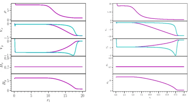
mean collisional time between ions and neutrals. Outflow boundary conditions are used except for symmetric boundary atx = 0. We run the simulation for two Mach numberM = 50 figure and M = 100 figure(1.13) which present the structure of neu-tral density neuneu-tral (red) and ion (bleu) velocity components, along the x direction before the jet reaches the outer boundary. We find agreement between the numerical and semi-analytical results [Mac Low, 1995] showing the softening behaviour of the C-shocks.

(48)

Figure 1.11: Structure of an oblique C shock with ambipolar diffusion MA = 5

(left panel), MA = 10 (right panel) and θ = π/4. The displayed shock values are

(ρ = 1 vx = 4.45, 9.47 vy = 0 Bx = √1₂ By = √1₂ p = 0.01). Profiles of neutral

density (magenta) and ion (cyan) velocity components obtained from the equation of relative drift velocity between ion and neutrals,vi = v + _γ_ad1_ρ_i_ρ(∇ × B) × B and

magnetic field components.

III.3.2 Alfven waves

Observed UV radiation of the accreting material in T tauri star is now believed to be entrained by magnetospheric field that releases its mechanical energy on the star surface [Matt and Pudritz, 2005]. Dissipation of Alfven waves on the stellar sur-face over magnetospheric accretion shocks constitute a good mechanism helping to launch outflow, building up a high enthalpy reservoir allowing thereby propagation of jets. [Kulsrud and Pearce, 1969] showed that ambipolar diffusion cause the

(49)

dissipa-III. Jet morphology

tion of the waves in a partially ionised plasma. Following [Choi et al., 2009] [Masson et al., 2012], we have examined the physics of propagating and damping of Alfven wave caused by ambipolar diffusion.

The simplest numerical implementation of Alfven wave evolution is a standing wave formed along the diagonal on thex_{− y plane, with initial velocity v}x = vy = 0

and vz = VampvAsin(2πx + 2πy). The initial peak amplitude is given by Vamp = 0.1,

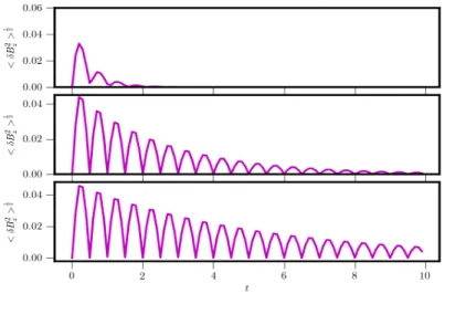
the background density and magnetic field have been set to be uniform withρ = 1 and B= B0ˆx. This gives the characteristic Alfven speedvA= √1₂, the wave number have

been set tokx= ky = 2π/L, the sound speed Cs = 1 with P = Cs2ρ = 1, we choose as

collisional coupling constants, γad = 1000, 500 and 100 with ρi = 0.1. For this test,

the boundary conditions are set to be periodic for x and y directions and outflow in the z direction. It has been done in a computational box of x = y = z = [0, L] with L = 1 using 1283 _{cells. The result is shown in figure (1.12); the time evolution}

of the spatially root mean square < δB2

z >1/2 for three different coupling constants

γad = 1000, 500, 100 top, bottom and middle respectively. The propagation of alfven

(50)

Figure 1.12: Time evolution of p< B2

z > , the root mean square of the magnetic

field in the z direction for γad = 1000 (top) , 500 (middle) and 100 (bottom) in the

test of Alfven waves with ambipolar diffusion.

III.4

Kelvin-Helmholtz instability

The contact discontinuity that separates shocked outflow material, which has passed through the Mach Disk, from shocked ambient material, which has passed through the bow shock, has different density and temperature but the same pressure. This pressure equilibrium prevents the material on each side of the discontinuity from mixing initially. It may later mix through the Kelvin-Helmholtz instability (KH hereinafter). In this region (labelled in figure (1.8) ) the jet beam acts as a resonant cavity for transverse subsonic acoustic waves confined within the interior of the beam. The acoustic waves must be subsonic otherwise they would create disruptive shock waves. Certain frequencies or modes become amplified and can grow into KH insta-bilities [Stone et al., 1997]. The KH is among the most relevant process occurring in outflow. It leads to the disruption of the jet and also drive the formation of pecular

(51)

III. Jet morphology

morphologies observed in stellar collimated object, its has been confirmed that KH is concentrated through hoop stress to form eddies (labelled in figure(III.3.2) [Trussoni et al., 1997a].

III.5

S-shape C-shape

Usually, the large scale morphology of parsec scale flows is characterised by a pre-cession of few degree Class (0/ I) jets (see e.g. Figure(1.13)) with typical periods ranging from 400 to 50000 years (e.g [Eisloffel et al., 1996]; [Devine et al., 1997]). This precession is characterised by either S-shape or C-shape: by an S-shape, point-symmetric with respect to the source, for numerical simulations see [Raga et al., 2009]. Such morphology can arise as a consequence of precession of either stellar spin axis or disk axis. Another morphology is C-shaped symmetry or Mirror sym-metric signature. Such precession is found in HH211 Class 0 jet, HH111 Class I jet, and the HH30 Class II jet, with orbital periods of 43 years, 1800 years and 114 years respectively [Lee et al., 2010]; [Noriega-Crespo et al., 2011]. Possible causes are deflection by a wind or motion of the source in the surrounding cloud eg jet from Herbig Be shows wiggles with 4_{− 8 years similar to the time scale of} its EXOr outbursts, suggesting that such outbursts may be driven by undetected companion [Whelan et al., 2010]. These effects in turn can be used as a signature of dynamical interactions in multiple star systems.

(52)

Figure 1.13: Top: C shape, the HH211 Class 0 molecular jet imaged with the SMA at0.3” _{resolution. The CO, SiO, SO, and 0.85 mm continuum are red, green, blue,}

and orange (contours), respectively. The jet is clearly seen on both sides of the source with more than one cycle of wiggle. The wiggle is reflection-symmetric about the source and can be reasonably fitted by an orbiting source jet model [Lee et al., 2010]. Bottom: S shape, three color spitzer IRAC image of the L1157 outflow blue 3.6 µm, green 4.5µm and red 8.0µm image taken from [Frank et al., 2014]

IV

Jet emission

Protostellar jets emit in spectral lines as well as continuous radiation and have been detected in all bands of the electromagnetic spectrum (exceptγ rays see [Bally et al., 2007]). In star forming regions, they are responsible for maser emission, free free, and synchortron radiation at radio wave lengths. As we discussed so far, one observed characteristic of jets is that a series of brightest features, emission knots (working surface) is seen [Mundt, 1986] rather than a continuous Laminar flow. The observed knotty emission occurs in shock regions where the gas within the jet is heated and compressed. This region is visible in near IR, optical, UV radiation and X-ray and

(53)

IV. Jet emission

emit in variety of lines, therefore are rich source for diagnostic. It has been estab-lished that optical line emission of HH objects is well estabestab-lished within radiative shock models [Raga et al., 1997]; [Hartigan et al., 2001]. These steady jet models were replaced by time dependent ones, and line prediction were obtained from time dependent radiative jet simulation [Raga et al., 2004]. Different processes have been invoked to explain line excitation mechanism: shocks [Hartigan et al., 1994], am-bipolar diffusion [Garcia et al., 2000], turbulent mixing layers model [Binette et al., 2000]. Another process has been proposed recently, and more recently X-ray heat-ing [Teşileanu et al., 2012] with shock velocities in range of 370 − 525km/s and temperature in the range of 106 _{− 10}7_{K in the post shock layers with pre shock}

densities 103 _{− 10}4_cm−3_{, based on the comparison of theoretical line ratio with the}

observed one. Discriminant line ratio diagrams between the different mechanism mentioned below; using [S II] λ 6731, 6716, [OI] λ 6300 and [NII] λ 6583 are pre-sented in figure (1.14 (a)(b)(c)(d))

In the top diagram that represents [NII]λ 6583 / [O I] λ 6300 vs [SII] λ 6731 / [O I] λ 6300 (figure (1.14) panel(a)(c)) the theoretical and observed ratios are in good agreement with the one predicted through shock models for both microjets and HH objects. In contrast for (ambipolar diffusion and mixing layers model) the ratios [NII]λ 6583/ [O I] λ 6300 is insufficient to obtain close agreement due to low ionisation. In the bottom diagram panel (b)(d), which plots [SII]λ 6716 λ 6731 vs [SII]λ 6731 / [O I] λ 6300. The line ratios are in close agreement within planar shock models. In contrast for (ambipolar diffusion and mixing layers model) the predicted line ratios are displaced to the left of the observed one. It appears that the dominant excitation mechanism down to30AU of the star is shocks both in jets and microjets indicating shock velocities in the range of 70− 100km/s and pre shocks densities decreasing away from the star in the range of 105 _{− 10}3_cm−3 _{and temperature of}

1_{− 3 10}4_{K. For X-ray excitation mechanism three doublets of [S II] 6716+6731 Å,}

(54)

Figure 1.14: Comparison of observed line ratios (symbols) in DG Tau microjet panel (a)(b) and jets +HH object panel (c)(d) with the theoretical predictions of line ratios as predicted from radiative shock model [Hartigan et al., 1994] (green curve). Turbulent mixing layers [Binette et al., 2000] (dashed curves), and ambipolar diffu-sion (solid line) [Garcia et al., 2000]. Taken from [Cabrit, 2002]

(55)

IV. Jet emission

ionisation included. The figure shows that the theoretical values are in agreement with the observed one only for short distances after the shocks for the first part of the redshifted jet from the RW Aurigae pair.

Figure 1.15: Log10 scale plot on the jet axis of line ratio with X-ray pre ionisation included (lines) in comparison with the observed line ratios (symbols) for the three doublets of [S II] 6716+6731 Å, [O I] 6300+6363 Å, and [N II] 6548+6583 Å [Teşileanu et al., 2012].

Teşileanu [Teşileanu et al., 2012] have found that 10_{− 20% of ionisation fraction} is necessary to obtain a closer agreement between observed brightness distribution and simulated one by considering only jet propagation region. The purpose of this thesis emphasise on testing this basic hypothesis by considering both the launching and large scale regions simultaneously and explore the effects of photoionisation on the post shock conditions in YSO jets; which is a further challenge because of large scale dynamical range simulation and observation. Our work is based on high spatial simulation that implies a large number of dynamical grid points (see chapter 4).

(56)

V

Jet physics

Stellar jet around young stellar objects (eg. from T Tauri stars) are sufficiently close, so that they can be used as "laboratories" to measure their proper motion, radial velocities and the location of the components on the plane of the sky with high angular resolution.

Many aspects of the protostellar outflow has been clarified as depicted in the table(1.1). Protostellar jets velocities are usually in the range100_{− 500 km/s with} lifetime of at least 2× 105 _{years, suggesting an extended size of 2 to 3 pc or even}

more on the sky. They are highly supersonic, with Mach numbers > 20 and are very well collimated, at least several hundred AU from their source. Observations show that most of jets from YSOs are associated with accretion disks. Indeed, they are accretion powered with jet kinetic power in range of 1030_{− 10}33 _erg/s;

the average mass fluxes within the jet is estimated to range between 10−7 _to ₁₀−9

Myears−1. Most protostellar jets are thought to be overdense, having a density

between10 and 20 times that of the ambient medium [Morse et al., 1992], [Reipurth and Bally, 2001], and in the range from 10 for the faintest object to 105 _cm−3

for the brightest [Reipurth and Bally, 2001]. With an increasing and sensitivity of angular resolution, large telescopes have revealed an average hydrogen jet number of 104 _cm−3 _{[Bacciotti et al., 1999],Typical temperature within the jet are in the range}

103 _to ₁₀4 _{K. Jets display a significant degree of ionisation which tends to decrease}

gradually as electrons recombine [Bacciotti et al., 1999]. Typical examples of such jets are HH30, HH34, HH47 and HH111.

(57)

V. Jet physics

Quantity Reference Values

Jet Kinetic power 1030_{− 10}33_erg/s

Jet Velocity 100_{− 500km/s}

Jet Mach number 20− 40

Ionisation fraction 2_{− 30%}

Jet electron number density 103_{− 10}4_cm−3

Length 0.01pc up to a few parsec (103_{− 10}5_)AU

Temperature 103_{− 10}4_K

Age 104− 105_years

Mass transport 10−9_{− 10}−7_M

/years

(58)

Chapter 2 The properties of YSO jets from

observations

What we observe is not nature itself, but nature exposed to our method of questioning

Werner Heisenberg

I

Origin of the Jet

The exact origin of the jet remains among unresolved problems. Indeed, jets find their origin in regions close to protostars (< 10 AU ) which require observations of high angular resolution, not yet achieved. However, HST observation of transverse velocity shifts inferred launching radii of0.2−3 AU [Bacciotti et al., 2002]; [Anderson et al., 2003]; [Coffey et al., 2004]. Among MHD models of jet formation three sites has been proposed to contribute to optical jets (disk, star and magnetosphere); see figure (2.1) that can coexist, i.e: more than one of these possibilities may be present in a given protostar outflow system [Ferreira et al., 2006].

(59)

I. Origin of the Jet

Figure 2.1: Global view of magnetised accretion ejection structure (MAES) around young star [Zanni and Ferreira, 2013]. Logarithmic density is displayed in color. Dashed lines represent Alfven surface SA (where Vp = Bp/4πρ ). The blue arrows

represent the poloidal speed. The magnetic field lines are traced in white. The yellow curves illustrate the three different components of jet launching namely: disk-wind, stellar-wind and magnetospheric-wind.

(60)

I.1 Disk-wind

In this model, the jet is launched either from an extended range radii or from narrow annulus near corotation, as sketched in figure (2.2) panels (a),(b) respectively. The outflow is powered by accretion and large scale magnetic field threading the disk. The ejection is magnetocentrifugal (for more details, see chapter 3). The total magnetic flux limit the radial extension of the ejection zones throughout the disk. In case of disk wind "D-wind" (r > 0.1AU ) (e.g. [Blandford and Payne, 1982]; [Wardle and Koenigl, 1993]; [Ferreira and Pelletier, 1995]; [Spruit, 2010]) such field may originate from the initial field, assumed to arise by advection of interstellar (fossil) magnetic field during the star formation that can be amplified by the dynamo effect. In the case where the ejection occurs only from one annulus in limited zone (re ≈ ri), one

gets an "X-wind"(e.g. [Shu et al., 1994]; [Shang et al., 2002]). It is important to highlight that disk wind models are self collimated and, in both cases, jets carry away the exact amount of angular momentum required to allow accretion in the underlying disk.

I.2 Stellar-wind

In this model the outflow is ejected from the surface of the star and its vicinity through an opens stellar magnetic field lines as illustrated in figure (2.2) panel (c). The magnetic field threads the innermost regions of the disk and channels the mate-rial, which forms accretion columns. The accreted matter crashes on the stellar sur-face dissipating their kinetic energy from accretion forming hotspots [Bouvier et al., 1995]. A large portion of this matter is re-ejected along the polar directions driven by pressure gradient thermally (e.g. [Sauty and Tsinganos, 1994]; [Sauty et al., 2002]) or from turbulent Alfven wave (e.g. [Hartmann and MacGregor, 1980]; [DeCampli, 1981] [Kwan, 1997]; [Camenzind, 1997]). The mass ejected along these directions has the fastest velocity and, carries highest angular momentum. The shock waves gener-ated by the accretion of matter and turbulence could explain the release of matter in

Étude de l’hydrodynamique stellaire moyennant le code PLUTO

T H É S E

Zoubida AHMANE

Étude de l’hydrodynamique stellaire moyennant le code

PLUTO

Simulation des effets de photoionisation sur les jets YSO

Study of stellar hydrodynamics using

PLUTO code

PhD joint with

Hadj Lakhdar Batna 1 University

Studi di Torino University

Zoubida AHMANE

T H E S I S

Zoubida AHMANE

Study of stellar hydrodynamics using PLUTO code

Simulations of protostar-driven photoionization in Herbig-Haro Jets

Abstract

Contents

List of Tables

List of Figures

Preface

Chapter 1

Introduction

I

Protostellar Outflows and Herbig-Haro Objects

II

Jets in the Context of Star Formation

II.1

Prestellar phase

II.2

Protostellar phase

II.3

Pre-main sequence phase

III

Jet morphology

III.1

Jet Beam

III.2

Bow shock - Working surface - Mach disk

III.3

Knots, hots-pots

III.4

Kelvin-Helmholtz instability

III.5

S-shape C-shape

IV

Jet emission

V

Jet physics

Chapter 2

The properties of YSO jets from

observations

I

Origin of the Jet

I.1

Disk-wind

I.2

Stellar-wind