HAL Id: hal-03225917
https://hal.archives-ouvertes.fr/hal-03225917
Submitted on 17 May 2021
HAL is a multi-disciplinary open access
archive for the deposit and dissemination of
sci-entific research documents, whether they are
pub-lished or not. The documents may come from
teaching and research institutions in France or
abroad, or from public or private research centers.
L’archive ouverte pluridisciplinaire HAL, est
destinée au dépôt et à la diffusion de documents
scientifiques de niveau recherche, publiés ou non,
émanant des établissements d’enseignement et de
recherche français ou étrangers, des laboratoires
publics ou privés.
Distributed under a Creative Commons Attribution| 4.0 International License
Dependence of Climate Sensitivity on the Given
Distribution of Relative Humidity
Stella Bourdin, Lukas Kluft, Bjorn Stevens
To cite this version:
Stella Bourdin, Lukas Kluft, Bjorn Stevens. Dependence of Climate Sensitivity on the Given
Distri-bution of Relative Humidity. Geophysical Research Letters, American Geophysical Union, 2021, 48
(8), �10.1029/2021GL092462�. �hal-03225917�
1. Introduction
The clear-sky response to an increase in greenhouse gases is a pillar of our understanding of global warm-ing (Charney et al., 1979; Manabe & Wetherald, 1967). It is generally believed that this response is better described by an atmosphere whose relative, rather than absolute, humidity remains constant with warming. The distinction is crucial because in an atmosphere where the relative humidity (RH) is fixed, the response of surface temperature to radiative forcing (e.g., from changing CO2), is roughly twice as large as would be the case should absolute humidity be fixed. In an influential review of these matters, Held and Soden (2000) presented theoretical arguments and evidence from modeling in support of a constant RH. At the time of their review, observations were insufficient to test this hypothesis, but Held and Soden concluded that “10 years may be adequate, and 20 years will very likely be sufficient, […] to convincingly confirm or refute the predictions.” It is now 20 years later.
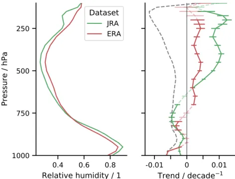
Taken at face value, two reanalyses of meteorological observations support this point of view, albeit less convincingly than we anticipated. This is shown in Figure 1, where above 600 hPa RH is increasing with warming, at a rate of 1%/decade to 4%/decade. Rather than attempting to establish the reliability of the trends—a task for which we lack expertize—our aim is to estimate their implication for how Earth's equi-librium climate sensitivity may be changing. How does a moister upper, or drier lower, troposphere make
Abstract
We study how the vertical distribution of relative humidity (RH) affects climate sensitivity, even if it remains unchanged with warming. Using a radiative-convective equilibrium model, we show that the climate sensitivity depends on the shape of a fixed vertical distribution of humidity, tending to be higher for atmospheres with higher humidity. We interpret these effects in terms of the effective emission height of water vapor. Differences in the vertical distribution of RH are shown to explain a large part of the 10%–30% differences in clear-sky sensitivity seen in climate and storm-resolving models. The results imply that convective aggregation reduces climate sensitivity, even when the degree of aggregation does not change with warming. Combining our findings with RH trends in reanalysis data shows a tendency toward Earth becoming more sensitive to forcing over time. These trends and their height variation merit further study.Plain Language Summary
Equilibrium Climate Sensitivity is the change in surface temperature in response to a doubling of atmospheric CO2. We study how the assumed vertical distribution of relative humidity affects this sensitivity. Theoretical considerations show that the more moist an atmosphere is, the more it warms as a response to an increase in CO2. Adding water vapor to the lower troposphere has the counter effect, lowering the sensitivity. We emphasize the importance of climate simulations taking humidity into account, as it is largely responsible for the difference in projections among models without clouds. We note surprising trends in humidity—with substantial drying of the lower troposphere over the ocean—in the last four decades as reported by two reanalyses of meteorological observations. Subject to the accuracy of these reconstructions, there appears to be a change with less moistening than expected, but with moistening/drying profiles which will condition Earth to become more sensitive to forcing over time. We stress the need for a study of observations to more critically evaluate these trends, and know better what models should aim for.© 2021. The Authors.
This is an open access article under the terms of the Creative Commons Attribution-NonCommercial License, which permits use, distribution and reproduction in any medium, provided the original work is properly cited and is not used for commercial purposes.
Dependence of Climate Sensitivity on the Given
Distribution of Relative Humidity
Stella Bourdin1,2 , Lukas Kluft1,3,4 , and Bjorn Stevens1
1Max Planck Institute for Meteorology, Hamburg, Germany, 2Laboratoire des Sciences du Climat et de l’Environnement,
LSCE/IPSL, CEA-CNRS-UVSQ, Université Paris-Saclay, Gif-sur-Yvette, France, 3International Max Planck Research
School on Earth System Modelling, Hamburg, Germany, 4Department of Earth Sciences, Faculty of Mathematics,
Informatics and Natural Sciences, Meteorological Institute, Universität Hamburg, Hamburg, Germany
Key Points:
• Climate sensitivity is sensitive to the assumed distribution of relative humidity (RH)
• Different RH profiles explain clear-sky climate sensitivity spread among models
• Tropical RH trend in reanalyses yields an increase in climate sensitivity
Supporting Information: Supporting Information may be found in the online version of this article. Correspondence to:
S. Bourdin,
Citation:
Bourdin, S., Kluft, L., & Stevens, B. (2021). Dependence of climate sensitivity on the given distribution of relative humidity. Geophysical Research
Letters, 48, e2021GL092462. https://doi. org/10.1029/2021GL092462
Received 18 JAN 2021 Accepted 25 MAR 2021
10.1029/2021GL092462
RESEARCH LETTER
Geophysical Research Letters
Earth more or less sensitive to forcing? Posing this question raises even more basic questions. For instance, to what extent does the given profile of RH matter for the clear-sky climate sensitivity, even if it remains constant with warming?
If the water vapor pressure, e, changes to keep RH constant with warming, then the fractional vapor pres-sure change is given by the Clausius-Clapeyron equation, as
v 2 v , e T e R T (1) with ℓv the vaporization enthalpy, Rv the water vapor gas constant, and T temperature. To the extent the radia-tive response to an increase in water vapor depends on its fractional change, as for instance is the case for well mixed greenhouse gases (Huang et al., 2016), Equation 1 predicts that this response—and hence the water vapor feedback—should be independent of RH. Support for this point of view is provided by observations and analyses that show outgoing long-wave radiation (OLR) varying linearly with T in a manner that is independ-ent of RH (Koll & Cronin, 2018; Zhang et al., 2020). These same studies show, however, that the robustness of this relationship is mostly a feature of a colder atmosphere. In the tropics, where continuum emission by water vapor in the 800 to 1,200 cm−1 spectral (window) region becomes more important, RH begins to color the relationship between OLR and T. The tropics cover a substantial portion of the Earth, which raises the question as to whether a sensitivity of the water vapor feedback to the given profile of RH might in part explain differences (15%, one sigma) in clear-sky feedbacks across climate models (Soden & Held, 2006; Vial et al., 2013), differences that are even larger across simulations designed to isolate the response of the tropical atmosphere to warming (Becker & Wing, 2020; Medeiros et al., 2008). Questions such as these have not been the topic of much study. Past work has focused on cloud changes (Sherwood et al., 2020; Stevens et al., 2016), to a degree that can give the impression that clouds alone stand in the way of a meaningful quantification of how surface temperatures, T, respond to radiative forcing. Exceptional is the study by Po-Chedley et al. (2018),
10.1029/2021GL092462
Figure 1. Mean profile (left) and linear trend over 40 years (solid, right) for ERA5 and JRA-55 reanalysis data. Error
bars show the 95% confidence interval for the gradient estimation. Lighter and dashed parts indicate levels for which the null hypothesis of the trend being zero has not been rejected (p-value > 0.01). The gray dashed line corresponds to what would be the trend in RH for a constant absolute humidity considering ERA5 tropical temperature trend. Details about the trend analysis are given in supporting information.
Geophysical Research Letters
who argue that changes in RH in the southern-hemisphere extra-tropics are a large source of model spread; here we emphasize how and why such effects are also substantial in the tropics.
The idea that the climate response is sensitive to the particular distribution of RH being held fixed, can be thought of as a form of state dependence. Perhaps for the reasons given above, most studies addressing this issue adopt a conceptual framework that only admit surface temperature as a state variable (Knutti et al., 2017; Meraner et al., 2013). So long as RH does not vanish, it plays no role.
In the present article we report on our investigation of the influence of RH on climate sensitivity using a 1D radiative-convective equilibrium (RCE) model, and highlight a phenomenon we call humidity–de-pendence. Such a model is attractive for our purposes because it captures (often with surprising fidelity) the behavior of more elaborated descriptions of the climate system in a physically transparent manner. In Section 2 we describe the model and methods. In Section 3 we compute the relative impact of a perturbation in the profile at different levels, as a function of RH. In Section 4 we simulate less idealized profiles of RH to understand and better quantify their effect on the spread in clear-sky climate sensitivity produced by more elaborated models. In Section 5 we return to the trends in the reanalysis RH to quantify their implications for our understanding of the clear-sky climate sensitivity. We conclude in Section 6.
2. Model and Methods
Calculations were performed using the 1D-RCE model konrad (Dacie et al., 2019; Kluft et al., 2019). We adopt a configuration that uses the RRTMG radiative scheme (Mlawer et al., 1997) and a hard convec-tive adjustment (Dacie, 2020) following the moist adiabatic lapse rate. Only clear-sky calculations are per-formed. In a subset of calculations discussed at the beginning of Section 3, we also used a uniform lapse rate. We used 500 pressure levels between 1,000 and 0.5 hPa. Following the prescription of the Radiative Convective Equilibrium Model Intercomparison Project(RCEMIP) (Wing et al., 2018), the solar constant is set to 551.58 W m−2 and the zenith angle to 42.05°, resulting in an insolation of 409.6 W m−2. The surface albedo is 0.2. The ozone profile is defined according to RCEMIP guidelines (Wing et al., 2018), with addi-tional coupling to the cold-point tropopause allowing the ozone layer to shift with troposphere deepening (Kluft, 2020). The RH follows a prescribed vertical distribution up to the cold-point above which the specific humidity is kept uniform at its cold-point value. The RH is defined with respect to saturation over water above 0°C and with respect to saturation over ice below −23°C. In between, a combination of both is used (ECMWF, 2018).
A run is defined by its RH profile. It is composed of two equilibrium computations: (i) a spin-up with a con-stant surface temperature T0 = 300 K, (ii) a new equilibrium after applying a sudden doubling of the CO2 concentration. In (ii) the surface has no longer a fixed temperature but a fixed enthalpy sink, whose value is the top of the atmosphere radiative imbalance at the end of the spin-up, as Kluft (2020) argues to be best practice. The equilibrium elimate sensitivity (ECS), of our model is defined as the difference between the second equilibrium surface temperature and T0.
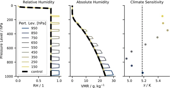
In Section 3, we discuss perturbation runs. In these, the tropospheric RH profile is uniform except for a 600 m thick layer, where the RH is increased or decreased (the perturbation). A perturbation run is thus defined by a base RH, a perturbation pressure, and a perturbation intensity δRH. The corresponding “run” without perturbation is called a control run. This is illustrated in Figure 2. Arithmetic changes in RH are adopted, as they correspond to geometric changes in absolute humidity, to which (as a first approximation) the radiative response is proportional, irrespective of the base RH.
As a measure of the impact of a perturbation, we define the amplification factor a as the ratio of the in the perturbation run, p, to the in the corresponding control run, c:
p
c 1.
a
(2) In reanalysis data, see Figure 1, the RH profiles peak in the boundary layer and in the upper-troposphere and show a distinct minimum in the mid-troposphere. For this reason, we call such a profile C-shaped. In
Geophysical Research Letters
order to simulate a C-shaped RH profile, we developed the following piecewise model, in pressure coordi-nates (shown in Figure 4):
- Linear in the boundary layer, from the surface to the lower-tropospheric peak (low point)
- Quadratic in the mid-troposphere, defined by 3 points: the two peaks and the humidity at 500 hPa (mid point)
- Linear above the upper-tropospheric peak, defined by the upper-tropospheric peak (top point) and the cold-point (which is more strongly coupled to T than p)
The advantages of such an RH profile is that it is defined by only 5 points, corresponding to parameters that are straightforward to interpret, and it catches the main feature of a realistic profile better than a uniform profile. Moreover, these parameters give us enough degrees of liberty to fit well AMIP and RCEMIP data, as detailed in Section 4.
3. Humidity–Dependence of
To understand how varies with mean RH, we first perform runs with different uniform tropospheric RH profiles, both for the case of uniform and moist adiabatic lapse rates. Values of for these runs are plotted in Figure 3 (top panel). We find a robust increase in with a moister troposphere. We decomposed into contributions from the forcing and the feedback following Gregory et al. (2004). This shows that changes in
arise from changes in feedback as the forcing tends to be much smaller and of the opposite sign.
Let us use the effective emission height concept for the interpretation of our calculations. Let Φe be Earth's infrared irradiance at the top of the atmosphere. It can be associated with radiant power emitted by a black body at a temperature, Te, such that Φe Te4, where σ is the Stefan-Boltzmann constant. We define the
effective emission height to be the altitude ze such that T(ze) = Te. These ideas can be generalized to allow for spectrally specific effective emission heights, which we denote ze,λ, as done by Seeley and Jeevanjee (2021). To help understand the water vapor feedback, we first apply this concept to a case with a uniform lapse rate, dT/dz = −Γ, and gray radiation characterized by a single emission height. If an initial (positive) perturba-tion in CO2 causes an increase in the emission height δze,i > 0, the troposphere (and surface) warms until
T(δze,i) = Te to maintain Φe. As a reaction to this warming, if RH is to remain fixed, the absolute humidity must increases following Equation 1. The fractional increase in water vapor partial pressure δe/e will in
10.1029/2021GL092462
Figure 2. Illustration of the perturbation runs method. The control run, with a base RH of 0.8, is shown in dashed
black. Each color corresponds to a run with a perturbation δRH = 0.2 at a different level. The two left panels show the relative and absolute humidity profiles. The right panel shows for each perturbation run as a function of perturbation pressure alongside the value of for the control run (dashed vertical line).
Geophysical Research Letters
turn lead to a further change in ze, which must be balanced by further warming, increasing humidity, and so on. , is the sum of the response from the initial forcing, plus this water vapor feedback.
The increase in with RH (Figure 3) calls into question the line of rea-soning (Section 1) leading to the expectation that is independent of RH. This may be indicative of continuum emission and absorption by water vapor in the window (800 to 1,200 cm−1) region, which increases nonlin-early with absolute humidity (Koll & Cronin, 2018). This would give rise to a stronger humidity-dependence of at high temperatures. We thus repeat our calculations at lower values of T0, at which the effect of the water vapor continuum is negligible. Reducing the working temperature progressively reduces the sensitivity to RH—at T0 = 288 K increases by only 25% as RH increases from 0.1 to 0.9—consistent with the hypothesis that the unexpected behavior does indeed stem from the effect of contin-uum emission in the window region.
The case of the moist adiabat (orange points and matrix in Figure 3) in-troduces additional complications. A property of the moist adiabat is that the lapse rate monotonically decreases with temperature. This gives rise to three effects: (i) as the atmosphere warms the mean lapse rate becomes smaller (lapse-rate feedback); (ii) for the same surface temperature and mean lapse rate, the moist adiabatic lapse rate is associated with a tem-perature profile that is everywhere warmer than for the uniform lapse rate; (iii) the lapse-rate is less than the mean in the warmer, lower, tropo-sphere but greater in the colder, upper, tropotropo-sphere. The first effect gives rise to a negative feedback with warming (smaller ) as it implies that the temperature at the emission height warms more rapidly than at the surface. The second effect gives rise to a positive feedback (larger ) be-cause a warmer atmosphere will (for the same RH) have a larger absolute humidity. The third effect implies a more bottom heavy humidity profile, which would suggest a slight reduction in .
At low absolute humidities the negative lapse-rate feedback dominates. This explains why in the upper panel of Figure 3, for RH ≤ 0.75, runs with a moist-adiabatic lapse rate have a substantially smaller . This difference be-comes even more pronounced (as expected) if one uses the integrated water vapor (IWV) as the control variable. For high humidities the second effect dominates. This occurs because for the chosen value of T0 the atmospheric window loses its transparency (Koll & Cronin, 2018), which is a self-ampli-fying effect that explains the sharp increase in . To test our explanation, we performed additional calculations with a smaller T0. As the above argument would anticipate, this reduces the sensitivity to RH (see Figure S3 in the supporting information), a result that is also consistent with a T0 decreasing with T0, for example, as shown by Meraner et al. (2013). Finally, calcula-tions (not shown) that adopt a constant moist adiabatic lapse rate (which cannot change with warming) also have a slightly reduced as compared to calculations adopting a uniform lapse rate for the same value of integrated water vapor (IWV). In this case, there is no lapse-rate feedback and the IWV is the same. This supports our inter-pretation of the third effect, whereby the shape of the humidity profile also influences .
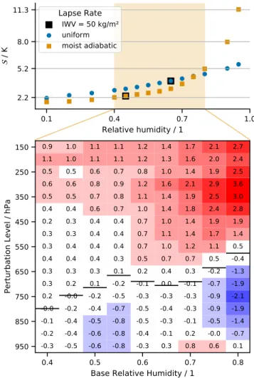
To assess how the shape of the RH profile influences we perform perturbation runs as described in Sec-tion 2 (see also Figure 2). Perturbation runs are performed with δRH = −0.1, +0.1, +0.2. From these the amplification factor, a per Equation 2, is related to δRH through linear regression. Figure 3 plots a from its regressed slope multiplied by δRH = 0.1. Values are calculated for RH perturbations applied every 50 hPa to an otherwise constant RH profile. This sequence of height varying perturbation runs is computed for 0.4 ≤ RH ≤ 0.8. The impact of a positive RH perturbation is small, but discernibly positive (increasing
10.1029/2021GL092462
Figure 3. (Upper panel) for different uniform tropospheric RH, and for experiments with a uniform tropospheric lapse rate of 6.5 K km−1 or with a
moist adiabatic lapse rate. Black squared points correspond to experiments were integrated water vapor (IWV) was the closest to 50 kg m−2. (Lower
panel) Amplification factor a (in percent) for 0.1 RH perturbation for different humidities and different perturbation levels. Blue and red colors for changes larger than 0.5% in magnitude are indicative of the value's range. Black lines represent the mid-tropospheric level at which a changes sign.
Geophysical Research Letters
) in the upper troposphere, and negative (decreasing ) in the lower troposphere. Simulations where the perturbations are fixed relative to the profile of T—which in the mid and upper troposphere is, following Romps (2014), likely to be a more realistic representation of RH—lead to weaker changes in , but imply a similar sensitivity to shape. Perturbations at lower values of p (equivalently lower T) lead to larger increas-es in . In every case, the higher the base RH, the stronger is the sensitivity to the humidity perturbation. Moreover, the level of sign change rises with base RH.
The perturbation runs are consistent with our earlier discussion, but not especially intuitive. To understand them, and test their robustness, we performed line-by-line radiative transfer using the ARTS model (Bue-hler et al., 2018), the results of which are provided graphically in the supporting information (Figure S2). We find two opposing effects. In spectral regions where ze,λ is near the height of the RH perturbation, the change in ze,λ as water-vapor adjusts to warming is lessened. It is as if the fixed perturbation height helps
10.1029/2021GL092462
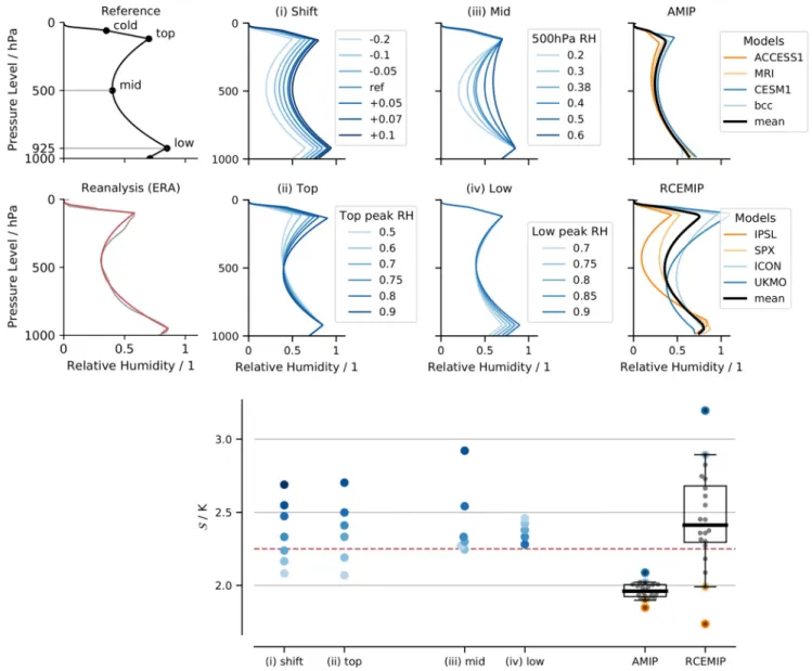
Figure 4. (Upper two rows) C-shaped relative humidity (RH) profiles: Reference 0.7/0.4/0.85 (top/mid/low) profile (top-left); ERA5 profile as computed
for Section 5 (gray), and corresponding C-shaped fit (red) (bottom-left). Four central panels correspond to the idealized experiments described in the first paragraph of Section 4. Two right-most panels display the mean and extreme profiles of the AMIP (top-right) and Radiative Convective Equilibrium Model Intercomparison Project (RCEMIP) (bottom-right) data sets. (Lower panel) for the idealized experiments and for the experiments with a profile fitted to the AMIP or RCEMIP ensembles. Boxplots’ whiskers are set to display the 5th and 95th percentiles. On this graph and for statistics, only one point per model “family” (i.e., issued by the same institute) is used, corresponding to the average of all this family's models. Red dashed line corresponds to the computed with ERA5 C-shaped fit RH profile above.
Geophysical Research Letters
anchor ze,λ. In spectral regions where the effective emission height is well below the RH perturbation, the change in ze,λ as water-vapor adjusts to warming is heightened—increasing the strength of the water vapor feedback. The first (damping) effect explains the reduction in associated with RH perturbations in the lower troposphere. It is also apparent at strongly absorbing wave numbers (rotational and ro-vibrational bands) for the perturbations in the upper troposphere. But for the latter case this reduction is more than offset by the second (amplifying) effect whereby the perturbation in the upper atmosphere increases the changes in ze,λ in parts of the window-region where CO2 does not dominate.
We call humidity–dependence the fact that the climate sensitivity depends on the RH. Not only does the sensitivity depend on the overall humidity, or IWV, but also on the distribution of humidity, that is the shape of the RH profile.
4. Implications for Model-Based Estimates of ECS
Given the nonlinearity of these effects, generalization is not automatic. Here, we check whether results of the previous section can also be identified for less idealized perturbations to RH profiles more similar to those observed and simulated by climate models. For this purpose, we use C-shaped RH profiles as defined in Section 2. To reduce their degrees of liberty we additionally fix the low point to 925 hPa and set the slopes below the low point, and above the high point, to 2.0 × 10⁻⁵ Pa−1 and −5.8 × 10⁻⁵ Pa−1, respectively. These values are the mean of the parameters when fitting to RCEMIP profiles (see following paragraphs). We additionally set the RH at the cold-point to be half its peak (upper-troposphere) value, the level of this cold-point being computed by konrad. Calculations (runs) were then performed to quantify the impact of changing the remaining parameters: Starting from a 0.7/0.4/0.85 (top/mid/low) profile, we: (i) shifted the whole profile; (ii) changed only the RH at the top of the atmosphere; (iii) changed only the humidity at 500 hPa; (iv) changed only the humidity in the lower atmosphere. Humidity profiles and resulting changes in are presented in Figure 4. Qualitatively the response to these perturbations agrees well with what was learned from the response to more idealized perturbations: (i and ii) increases with an increase in the upper tropospheric RH, also when this is part of a general moistening; (iv) decreases if RH increases are confined to the lower troposphere; and (iii) increases in RH in the middle troposphere lead to little change in until a critical RH (associated with the closing of the window) is reached, at which point begins to increases markedly. The same set of experiments have been performed with a C-shaped profile invariant in
T in the upper-troposphere, to find very similar results (not shown).
In a second step, we performed runs with RH profiles set to fit RCEMIP simulations using storm-resolving and general circulation models (Except for UKMO-CASIM whose humidity profile led to a runaway) on large domains with an SST of 300 K (Wing et al., 2020) and CMIP5 AMIP ensembles. The fit is done by retrieving the pressure and humidity of the five points defining our C-shaped profile. In particular, the low and top points coincide with the local maxima and the cold-point pressure is retrieved from the temperature profile. The mid point remains fixed at 500 hPa and the surface is taken as the lowest point available. This enables us to assess the effect of the humidity profile alone, all other things being equal.
With RCEMIP RH profiles, we find a ± 26% variation around the mean value. The spread in feedback is −1.25 to −3 W m−2 K−1, slightly smaller but comparable to what is found by Becker and Wing (2020). We thus explain the surprisingly large spread in clear-sky sensitivity in RCEMIP as being in large part a response to different RH profiles simulated by the models. Both differences in the IWV and the shape of the profiles contribute to the spread, the latter more so, as is also evident by comparing sensitivities calculated using ICON versus the UKMO RH profiles. To the extent that the inter-model spread in RH to different de-grees of convective self-aggregation, as claimed by Becker and Wing (2020), our work suggests that different degrees of convective self-aggregation can influence the climate sensitivity, even if the convective self-aggre-gation does not change with warming.
From CMIP5 AMIP output, we retrieved mean profiles over the tropical oceans (equatorward of 30°) aver-aged over the entire simulated period. As compared to RCEMIP RH profiles, those from the AMIP simula-tions are on average dryer, and thereby associated with a smaller . The drier AMIP profiles are indicative of large-scale circulations driven by differences in surface temperatures, i.e., Hadley and Walker cells which
Geophysical Research Letters
give rise to the dry tropics. The AMIP simulations differ less in their humidity profiles and likewise show less spread in , but even so differences approaching 10% are evident.
Given observations of the RH profiles in the atmosphere, it should be possible to correct model estimates of climate sensitivity using calculations such as ours. From a comparison of Figures 1 and 4, we note that the RCE models tend to be moister than the observations, the AMIP simulations are drier. Fitting the C-shaped humidity profile to the observations yields an of about 2.25 K; this is smaller than that of most RCE mod-els, but larger than for the AMIP models. Likewise, ECS estimates in early calculations following the RH humidity profile used by Manabe and Wetherald (1967), would, due to an unrealistically dry upper atmos-phere, be biased too low. However, for the lower humidities and temperatures used in that study, the fixed lapse assumption actually over compensates, leading to a larger sensitivity as seen in Kluft et al. (2019). This, along with the upper panel of Figure 3, is illustrative of how the lapse rate feedback depends on the base state RH.
5. Impact of RH Trends in Reanalysis Data
Based on the above analysis we return to our initial question, which is how to interpret RH trends in the reanalysis products. The profiles presented in Figure 1 are from the ERA5 (Hersbach et al., 2020), and the JRA-55 (Kobayashi et al., 2015) reanalyses of the past 40 years (1979–2019) of meteorological observations. Relative and absolute humidity, as well as temperature, are averaged over tropical oceans (equatorward of 30°). Trends regressed from monthly data are significant at several levels and consistent across both rea-nalyses. They are also evident in the difference between the mean profile in the first and last decade (not shown). We were surprised that RH at low levels was robustly decreasing—something that merits further investigation—even if averaged over height δRH ≈ 0. Our analysis does not tell us how strongly these trends influence the expected warming over the past 40 years, but it does tell us that the pattern of change, with moistening aloft and drying in the lower middle troposphere is conditioning the climate system toward greater sensitivity.
6. Conclusions
The response of the atmosphere to radiative forcing as a function of the assumed profile of RH is explored using a one-dimensional RCE model. For profiles chosen to sample the range produced by state of the art climate and storm-resolving models run under idealized conditions, the calculated equilibrium climate sen-sitivity of our model () varies between 2 K and 3 K, depending on the RH profile, highlighting a humidity– dependence of the climate sensitivity: Moister atmospheres were shown to have a larger , increasingly so with warmer temperature, consistent with understanding of how water vapor influences the transmissivity of the atmospheric window (Koll & Cronin, 2018; Nakajima et al., 1992; Seeley & Jeevanjee, 2021). is further shown to increase with increasing humidity in the upper troposphere, but decreases with increases in humidity in the lower mid-troposphere.
The use of a simple physical model, konrad, makes it easier to understand the basic physics determining the outcome of our calculations. For instance, with the chosen framework it is possible to show how the lapse rate's influence on the total amount and vertical distribution of humidity for a given profile of RH influenc-es . We could also investigate how depends on the shape of the RH profile, which expresses competing effects, whereby perturbations to the humidity can both reduce or increase the change in the emission height associated with changes in absolute humidity to maintain a constant RH with warming. The former effect dominates when the humidity perturbation is near the emission height resulting in a slight reduction in for bottom heavy humidity profiles.
Our work emphasizes the importance of realistically representing the RH profile when calculating climate sensitivity. Models that are too humid, particularly in the mid- and upper-troposphere will have larger sen-sitivities, an effect which will amplify with increased warming. Convective self-aggregation modifies the mean RH profile, thereby reducing ECS, even if the degree of convective aggregation itself does not change with warming. In this context, our study also encourages the use of RH as metric of the fidelity of the moist
Geophysical Research Letters
physics in climate models. To the extent climate models are unable to realistically represent the observed distribution of RH, our methods may make it possible to estimate the quantitative effect of these biases. Humidity profiles over tropical oceans as represented in reanalysis products, tend to be moister than those produced by models forced with observed SSTs, implying a larger clear-sky sensitivity. Three dimension-al radiative convective equilibrium models, which are more physicdimension-al—but less constrained by large-scdimension-ale sea-surface temperature gradients—tend to be more humid, but also have more divergent humidity profiles. Surprisingly large changes in RH are reported by the reanalysis products over the last 40 years, changes which our calculations suggest will condition the climate system to be more sensitive to forcing in the future. This finding adds an additional dimension to Knutti and Rugenstein's (2015) statement that the feedback parameter is not constant, and that nonlinearity in the system may be important when assessing Earth's equilibrium climate sensitivity. The surprising trends in the reanalysis humidity products, particu-larly the drying in the tropical lower troposphere, reminds us of Held and Soden's plea to be attentive to this issue, and merits the renewed attention of experts.
Conflict of Interest
The authors declare no conflict of interest.
Data Availability Statement
Primary data including simulation scripts and code for reproducing the figures are available on Zenodo through https://doi.org/10.5281/zenodo.4559581; konradv0.8.1 is available at github.com/atmtools/konrad, and latest sources are available at https://doi.org/10.5281/zenodo.4434837; ERA5 data is available on the Copernicus Climate Change Service Climate Data Store (CDS, https://cds.climate.copernicus.eu/cdsapp#!/ dataset/reanalysis-era5-pressure-levels-monthly-means?tab=overview); JRA-55 data were retrieve from https://jra.kishou.go.jp/JRA-55/index_en.html; The German Climate Computing Center (DKRZ) hosts the standardized RCEMIP and CMIP5-AMIP output (https://cera-www.dkrz.de/WDCC/ui/cerasearch/ info?site=RCEMIP_DS).
References
Becker, T., & Wing, A. A. (2020). Understanding the extreme spread in climate sensitivity within the radiative-convective equi-librium model intercomparison project. Journal of Advances in Modeling Earth Systems, 12(10), e2020MS002165. https://doi. org/10.1029/2020MS002165
Buehler, S. A., Mendrok, J., Eriksson, P., Perrin, A., Larsson, R., & Lemke, O. (2018). ARTS, the atmospheric radiative transfer simulator— version 2.2, the planetary toolbox edition. Geoscientific Model Development, 11(4), 1537–1556. https://doi.org/10.5194/gmd-11-1537-2018
Charney, J. G., Arakawa, A., Baker, D. J., Bolin, B., Dickinson, R. E., Goody, R. M., et al. (1979). Carbon dioxide and climate: A scientific
assessment. National Academy of Sciences.
Dacie, S. (2020). Using simple models to understand changes in the tropical mean atmosphere under warming. University of Hamburg. (Unpublished doctoral dissertation).
Dacie, S., Kluft, L., Schmidt, H., Stevens, B., Buehler, S. A., Nowack, P. J., et al. (2019). A 1D RCE study of factors affecting the tropical tropopause layer and surface climate. Journal of Climate, 32(20), 6769–6782. https://doi.org/10.1175/JCLI-D-18-0778.1
ECMWF. (2018). Part IV: Physical processes. In IFS documentation CY45R1. ECMWF. Retrieved from https://www.ecmwf.int/node/18714
Gregory, J. M., Ingram, W. J., Palmer, M. A., Jones, G. S., Stott, P. A., Thorpe, R. B., et al. (2004). A new method for diagnosing radiative forcing and climate sensitivity. Geophysical Research Letters, 31(3), L03205. https://doi.org/10.1029/2003GL018747
Held, I. M., & Soden, B. J. (2000). Water vapor feedback and global warming. Annual Review of Energy and the Environment, 25(1), 441.
https://doi.org/10.1146/annurev.energy.25.1.441
Hersbach, H., Bell, B., Berrisford, P., Hirahara, S., Horányi, A., Muñoz-Sabater, J., et al. (2020). The ERA5 global reanalysis. Quarterly
Journal of the Royal Meteorological Society, 146(730), 1999–2049. https://doi.org/10.1002/qj.3803
Huang, Y., Tan, X., & Xia, Y. (2016). Inhomogeneous radiative forcing of homogeneous greenhouse gases. Journal of Geophysical Research:
Atmospheres, 121(6), 2780–2789. https://doi.org/10.1002/2015JD024569
Kluft, L. (2020). Benchmark calculations of the climate sensitivity of radiative-convective equilibrium. Doctoral dissertation Universität Ham-burg. https://doi.org/10.17617/2.3274272
Kluft, L., Dacie, S., Buehler, S. A., Schmidt, H., & Stevens, B. (2019). Re-examining the first climate models: Climate sensitivity of a modern radiative-convective equilibrium model. Journal of Climate, 32, 8111–8125. https://doi.org/10.1175/JCLI-D-18-0774.1
Knutti, R., & Rugenstein, M. A. A. (2015). Feedbacks, climate sensitivity and the limits of linear models. Philosophical Transactions of the
Royal Society A Mathematical, Physical and Engineering Sciences, 373(2054), 20150146. https://doi.org/10.1098/rsta.2015.0146
Knutti, R., Rugenstein, M. A. A., & Hegerl, G. C. (2017). Beyond equilibrium climate sensitivity. Nature Geoscience, 10(10), 727–736.
https://doi.org/10.1038/ngeo3017
10.1029/2021GL092462
Acknowledgments
The research is supported by public funding to the Max Planck Society. S. Bourdin also benefited from the French state aid managed by the ANR under the ”Investissements d’avenir” programme with the reference ANR-11-IDEX-0004—17-EURE-0006. B. Stevens and L. Kluft acknowledge support from the European Union's Horizon 2020 Research and Innovation Programme under grant agreement No. 820829 (CONSTRAIN Project). The authors thank Tobias Becker, Sally Dacie, Didier Paillard, Maria Rugenstein, and Catherine Stauffer for helpful scholar discussion concerning this study, and Hauke Schmidt's GCC group at MPI-M for advice and feedback. The authors are also grateful to Sébastien Fromang and Theresa Lang for their review of an earlier version of this manuscript, as well as the stimulating and thoughtful comments of Nadir Jeevanjee and an anonymous reviewer, which led to a deeper understanding of our results.
Geophysical Research Letters
Kobayashi, S., Ota, Y., Harada, Y., Ebita, A., Moriya, M., Onoda, H., et al. (2015). The JRA-55 reanalysis: General specifications and basic characteristics. Journal of the Meteorological Society of Japan, 93(1), 5–48. https://doi.org/10.2151/jmsj.2015-001
Koll, D. D. B., & Cronin, T. W. (2018). Earth's outgoing longwave radiation linear due to H2O greenhouse effect. Proceedings of the National Academy of Sciences of the United States of America, 115(41), 10293–10298. https://doi.org/10.1073/pnas.1809868115
Manabe, S., & Wetherald, R. T. (1967). Thermal Equilibrium of the atmosphere with a given distribution of relative humidity. Journal of
the Atmospheric Sciences, 24, 241–259. https://doi.org/10.1175/1520-0469(1967)024〈0241:TEOTAW〉2.0.CO;2
Medeiros, B., Stevens, B., Held, I. M., Zhao, M., Williamson, D. L., Olson, J. G., & Bretherton, C. S. (2008). Aqua planets, climate sensitivity, and low clouds. Journal of Climate, 21(19), 4974–4991. https://doi.org/10.1175/2008JCLI1995.1
Meraner, K., Mauritsen, T., & Voigt, A. (2013). Robust increase in equilibrium climate sensitivity under global warming. Geophysical
Re-search Letters, 40(22), 5944–5948. https://doi.org/10.1002/2013GL058118
Mlawer, E. J., Taubman, S. J., Brown, P. D., Iacono, M. J., & Clough, S. A. (1997). Radiative transfer for inhomogeneous atmospheres: RRTM, a validated correlated-k model for the longwave. Journal of Geophysical Research, 102(D14), 16663–16682. https://doi. org/10.1029/97JD00237
Nakajima, S., Hayashi, Y.-Y., & Abe, Y. (1992). A study on the "runaway greenhouse effect" with a one-dimensional radiative-convec-tive equilibrium model. Journal of the Atmospheric Sciences, 49(23), 2256–2266. https://doi.org/10.1175/1520-0469(1992)049〈2256:A SOTGE〉2.0.CO;2
Po-Chedley, S., Armour, K. C., Bitz, C. M., Zelinka, M. D., Santer, B. D., & Fu, Q. (2018). Sources of intermodel spread in the lapse rate and water vapor feedbacks. Journal of Climate, 31(8), 3187–3206. https://doi.org/10.1175/JCLI-D-17-0674.1
Romps, D. M. (2014). An analytical model for tropical relative humidity. Journal of Climate, 27(19), 7432–7449. https://doi.org/10.1175/ jcli-d-14-00255.1
Seeley, J. T., & Jeevanjee, N. (2021). H2O windows and CO2 radiator fins: A clear-sky explanation for the peak in equilibrium climate
sen-sitivity. Geophysical Research Letters, 48, e2020GL089609. https://doi.org/10.1029/2020GL089609
Sherwood, S. C., Webb, M. J., Annan, J. D., Armour, K. C., Forster, P. M., Hargreaves, J. C., et al. (2020). An assessment of Earth's climate sensitivity using multiple lines of evidence. Reviews of Geophysics, 58, e2019RG000678. https://doi.org/10.1029/2019RG000678
Soden, B. J., & Held, I. M. (2006). An assessment of climate feedbacks in coupled ocean-atmosphere models. Journal of Climate, 19(14), 3354–3360. https://doi.org/10.1175/JCLI3799.1
Stevens, B., Sherwood, S. C., Bony, S., & Webb, M. J. (2016). Prospects for narrowing bounds on Earth's equilibrium climate sensitivity.
Earth's Future, 4(11), 512–522. https://doi.org/10.1002/2016EF000376
Vial, J., Dufresne, J.-L., & Bony, S. (2013). On the interpretation of inter-model spread in CMIP5 climate sensitivity estimates. Climate
Dynamics, 41(11), 3339–3362. https://doi.org/10.1007/s00382-013-1725-9
Wing, A. A., Reed, K. A., Satoh, M., Stevens, B., Bony, S., & Ohno, T. (2018). Radiative-convective equilibrium model intercomparison project. Geoscientific Model Development, 11, 793–813. https://doi.org/10.5194/gmd-11-793-2018
Wing, A. A., Stauffer, C. L., Becker, T., Reed, K. A., Ahn, M.-S., Arnold, N. P., et al. (2020). Clouds and convective self-aggregation in a multimodel ensemble of radiative-convective equilibrium simulations. Journal of Advances in Modeling Earth Systems, 12(9), e2020MS002138. https://doi.org/10.1029/2020ms002138
Zhang, Y., Jeevanjee, N., & Fueglistaler, S. (2020). Linearity of outgoing longwave radiation: From an atmospheric column to global climate models. Geophysical Research Letters, 47(17), e2020GL089235. https://doi.org/10.1029/2020GL089235