Getting high added-value from sampling

(1)

OATAO is an open access repository that collects the work of Toulouse

researchers and makes it freely available over the web where possible

Any correspondence concerning this service should be sent

to the repository administrator:

tech-oatao@listes-diff.inp-toulouse.fr

This is an author’s version published in: http://oatao.univ-toulouse.fr/25368

To cite this version:

Lyman, Geoffrey and Bourgeois, Florent

Getting high added-value from

sampling. (2015) TOS Forum, 2013 (1). 93-100. ISSN 2053-9681

Official URL :

https://doi.org/10.1255/tosf.46

(2)

Issue 5 2015

93 TOS

f o r u m

www.impublications.com/wcsb7

Getting high added-value from sampling

F.S. Bourgeoisa,b

and G.J. Lymanb

a_{Université de Toulouse, Laboratoire de Génie Chimique, Toulouse, France. E-mail:}_{florent.bourgeois@inp-toulouse.fr} b_{Materials Sampling & Consulting Pty Ltd, Southport, Queensland, Australia. E-mail:}_{glyman@iprimus.com.au}

Determination of the complete sampling distribution (Lyman, 2014), as opposed to estimation of the sampling variance, represents a significant advance in sampling theory. This is one link that has been missing for sampling results to be used to their full potential. In particular, access to the complete sampling distribution provides opportunities to bring all the concepts and risk assessment tools from statistical process control (SPC) into the production and trading of mineral commodities, giving sampling investments and results their full added-value. The paper focuses on the way by which sampling theory, via the complete sampling distribution, interfaces with production and statistical process control theory and practice. The paper evaluates specifically the effect of using the full sampling distribution on the Operating Characteristic curve and control charts’ Run Length distributions, two SPC cornerstones that are essential for quality assurance and quality control analysis and decision-making. It is shown that departure from normality of the sampling distribution has a strong effect on SPC analyses. Analysis of the Operating Characteristic curve for example shows that assumption of normality may lead to erroneous risk assessment of the conformity of commercial lots. It is concluded that the actual sampling distribution should be used for quality control and quality assurance in order to derive the highest value from sampling.

Introduction

A

ny engineering, quality or business analysis that deals with a real situation seeks to quantify a performance indicator and its associated uncertainty. This uncertainty comes from the propagation of the uncertainties associ-ated with all the variables that contribute to the analysis. Sampling is concerned with providing the user with the uncertainty about any property of a commercial lot that cannot be observed fully.

Sampling is the starting point for anything that has to do with analysis and improvement of engineering, quality and commerce in the production and trading of minerals. The added-value of sam-pling comes not from the samsam-pling itself, but from the use to which sampling data are put. Of course, the added-value of sampling is entirely dictated by the quality of sampling.

While estimation of sampling variance for the grade of a com-mercial lot is one important objective pursued by sampling theory, it must be remembered that sampling grade is a random variable. Tracking the variance only of this random variable implies that one assumes normality, which could lead to erroneous analyses and decisions once sampling data are put to the purpose for which they have been acquired should such an assumption be untrue. At any rate, it is always preferable to use the full sampling distribution over the sampling variance. The sole objective of this paper is to illustrate this point, through examples related to production control, quality assurance and quality control.

The assumption one has to make in order to use sampling data to any practical end, once sampling variance has been estimated using accepted sampling theory, is that the underlying full sam-pling distribution is Gaussian. It is difficult to ascertain whether this assumption is sound, and one may claim that it is perhaps so 80% of the time. In some situations, it is not the case (Venter, 1982). Recently, Lyman (2014, 2015) has shown that it is possible to esti-mate the full sampling distribution from sampling measurements, so that the limitation associated with the normality assumption can now be lifted altogether.

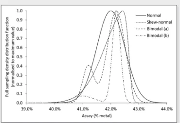
Figure 1 gives four distributions with identical mean

m

= 42% and standard deviation

s

= 0.5%, which will be used throughout the paper. These distributions represent realistic sampling distributions,

some of which exhibit skewness and bimodality. Standard sampling theory would state that these distributions are one and the same as their variances are equal, which implies that they should yield identi-cal downstream analysis and decision-making.

The results presented in this paper show that not only it is imper-ative that the full sampling distribution be estimated and used in order to get the maximum added-value from sampling, but that assuming a Gaussian sampling distribution can lead to erroneous and damaging analysis and decision-making.

The paper makes compelling arguments for using the actual full sampling distribution to get the full added-value of sampling, by examining three major uses of sampling data:

1. Production control, by looking at grade variation during the mak-ing of a commercial lot.

2. Quality assurance, with the Operating Characteristic curve (OC curve) as a risk analysis and decision-making tool for the con-formity of commercial lots.

Figure 1. Four distributions with identical mean

m

= 42% and stand-ard deviation

s

= 0.5%. The skew-normal distribution has parameters

a

= –8,

x

= 42.65%,

w

= 0.82%. The bimodal (a) and (b) distributions have parameters

a

= 0.2,

m

1 = 41.20%,

s

1 = 0.20%,

m

2 = 42.20%,

s

2 = 0.32% and

a

= 0.17,

m

1 = 41.00%,

s

1 = 0.40%,

m

2 = 42.20%,

(3)

Issue 5 2015

94 www.impublications.com/wcsb7

TOS

f o r u m

3. Quality control, with the Run Length (RL) distribution of control charts used for monitoring quality during production or in the laboratory.

Full sampling distribution and production

control

Sampling can be used for optimising the revenue during production of a lot. In particular, sampling should be used to optimise shipment grade during production of metal concentrates, by ensuring that commercial lots contain the maximum amount of valueless material acceptable under the terms of the client’s contract. This optimiza-tion requires knowledge of the full sampling distribuoptimiza-tion.

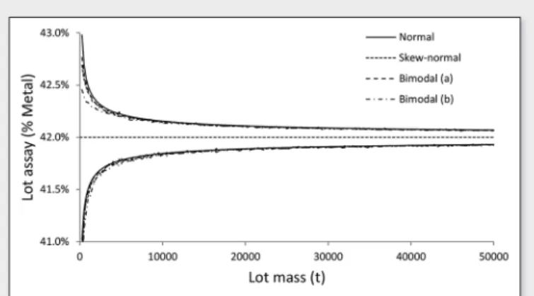
Figure 2 shows the 95% confidence interval for a 50000 t ship-ment loaded at a rate of 500 tph, sampled every 250 t for all four sampling distributions from Figure 1. The sampling distributions are assumed not to change during the making of the commercial lot.

In all cases, the narrowing confidence interval is a direct con-sequence of the propagation of variance from one sample to the next. Given that 200 samples are taken during the mak-ing of the lot, all four samplmak-ing distributions yield the same final sampling uncertainty, as per the central limit theorem. With the example shown, the 95% confidence interval of the lot assay is ±1.96(0.5%/

Ö

200) = 0.07% absolute. The 95% confidence inter-vals differ between the sampling distributions only at the start of the making of the lot. The differences are small with the example chosen, whose RSD = (0.5% / 42%) = 0.12% only. As expected, after approximately n = 50 sampling assays, all four sampling distri-butions converge toward

0.5% 42%, n æ _ö÷ ç Àçç_èm= s= ÷÷÷_ø. <Eq A>

It is worth noting that the width of the confidence interval, as well as the rate at which it narrows during the making of a lot, can be improved by improving sampling precision and increasing sampling frequency respectively.

From the point of view of production control during the making of a lot, the data that have been presented indicate that knowledge of the full sampling distribution is not necessary for quantifying the precision of the final lot assay, provided a sufficient number of samples (more than 50) are taken during the making of the lot. If one wants to use a small number of samples during the making of a lot, and yet make a correct estimation of the precision of the final lot assay, knowledge of the actual sampling distribution would be necessary. When considering that the loading of a commercial shipment may involve say 200 increments that are combined into 1 to 10 partial samples, using the full sampling distribution for assessment of shipment grade uncertainty is significant. Knowledge of the full sampling distribution would also prove useful should one want to optimise grade control during the making of a lot, since different sampling distributions will yield a different grade confidence interval at the beginning of the making of the lot.

Full sampling distribution and quality assurance

The Operating Characteristic curve, or OC curve, is the main risk analysis tool for practical acceptance sampling (Shmueli, 2014). It quantifies the conformity of a lot, by putting a number on the probability of accepting (alt. rejecting) a lot as a function of the true (un-known) assay of the lot and an Acceptance Quality Level (AQL). The OC curve truly is a sampling plan’s fingerprint, in that two distinct sampling schemes yield different OC curves. The OC curve is relevant to both the consumer and the producer, and it is widely used throughout the manufacturing industry and the food industry. The minerals industry however does not appear to make much use of the concept at the present time.

The OC curve has been accepted and is being used by the food industry as a key food safety risk analysis tool for mycotoxins in cereal grains (FAO, 2014; Bourgeois and Lyman, 2012; Lyman et al., 2011). The similarities between sampling mycotoxins in cereal grains in the food industry and sampling valuable metals in mineral concentrates in the minerals industry implies that the OC curve should also be of significant value to the trading of mineral commodities, and ought to be developed as a minerals trading risk analysis tool.

The link between sampling and the OC curve

Construction of the OC curve, for a given sampling plan, requires access to the full sampling distribution. This may partially explain why it has not been developed in the minerals industry, as it is only recently that a solution for estimating the full sampling distribution has been published (Lyman, 2014). This however is a partial explanation only, as it is possible to estimate the OC curve from estimation of sampling variance from standard sampling theory, under the assumption of normality of the sampling distribution.

The basic elements for constructing and interpreting an OC curve are briefly presented hereafter. Quantifying the risk of accepting or rejecting a lot with a true (unknown) assay requires that one defines an Acceptance Quality Level (AQL), which may be a Lower Ac-ceptance Quality Level (LAQL), an Lower AcAc-ceptance Quality Level (UAQL) or both. A supplier may want for example to produce a shipment of metal-bearing concentrate that bears no less than 41% metal, and no more than 43% metal. Depending on the AQL levels, the probability P_a of accepting the lot from sampling is calculated from the cumulative sampling distribution FX according to:

( ) ( ) ( ) ( ) : only : 1 only : a X X a X a X

LAQL X UAQL P x UAQL x LAQL X LAQL P x LAQL X UAQL P x UAQL F F F F £ £ = = - = ³ = - = £ = = <Eq B>

Let us assume that the lot, whose true (unknown) assay is 42%, is characterized by a full sampling distribution FX = À(m = 42%,

s = 0.5%), and that LAQL = 41% is the quality acceptance level criterion of interest. The probability of accepting the lot is then Pa = 1 – À(X = 41% | m = 42%, s = 0.5%) = 97.73%. The acceptance probability can be calculated for any true (unknown) value m of

the lot assay, which yields the OC curve.

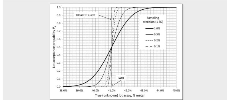
The dotted line in Figure 3 is the ideal OC curve, which corresponds to a sampling distribution with a variance equal to zero. This ideal case yields a lot acceptance probability strictly equal to 0 or 1 on either side of the AQL. In practice, there will always be a finite probability of accepting a non-conforming lot, or rejecting a conforming lot, for any true (unknown) assay of the lot. The steepness of the OC curve is entirely dictated by the nature of the sampling distribution, in particular its skewness, and by its variance, which is a measure of sampling precision. The effect of sampling variance s2_{on the steepness of the OC curve is illustrated in Figure 4, for}

FX = À(42%, s%).

The OC curve gives the actual value of the acceptance probability, which in turn quantifies the risk of accepting a non-conforming lot or rejecting a conforming lot. The OC curve is therefore a powerful risk management and decision making tool, whose construction relies entirely on the full sampling distribution.

The full sampling distribution and the OC curve

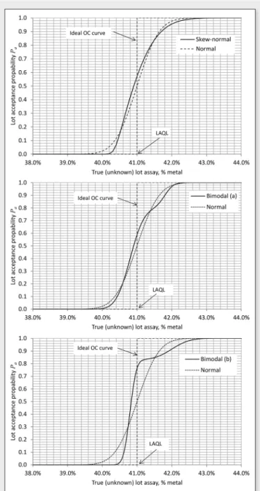
Figure 5 shows the OC curves obtained with the sampling distributions of Figure 1. It is recalled that all four sampling distributions share the same mean m = 42% and standard deviation s = 0.5%. In all cases, the acceptance quality level used to calculate the OC curves is set to LAQL = 41%.

The first observation is that the OC curves calculated using the non-Gaussian sampling distributions are all different from the one obtained with the Gaussian sampling distribution. The OC curve being the basis for quality assurance, it is concluded that the actual full sampling distribution must be used whenever sampling results are to be used for quality assurance purposes.

It is found that both the skewness and the bimodality of the sampling distributions have a significant effect on the OC curve. For the

From the point of view of production control during the making of a lot, the data that have been presented indicate that knowledge of the full sampling distribution is not necessary for quantifying the pre-cision of the final lot assay, provided a sufficient number of samples (more than 50) are taken during the making of the lot. If one wants to use a small number of samples during the making of a lot, and yet make a correct estimation of the precision of the final lot assay, knowledge of the actual sampling distribution would be necessary.

When considering that the loading of a commercial shipment may involve say 200 increments that are combined into 1 to 10 partial samples, using the full sampling distribution for assessment of ship-ment grade uncertainty is significant. Knowledge of the full sampling distribution would also prove useful should one want to optimise grade control during the making of a lot, since different sampling distributions will yield a different grade confidence interval at the beginning of the making of the lot.

Full sampling distribution and quality

assurance

The Operating Characteristic curve, or OC curve, is the main risk analysis tool for practical acceptance sampling (Shmueli, 2014). It quantifies the conformity of a lot, by putting a number on the probability of accepting (alt. rejecting) a lot as a function of the true (unknown) assay of the lot and an Acceptance Quality Level (AQL). The OC curve truly is a sampling plan’s fingerprint, in that two dis-tinct sampling schemes yield different OC curves. The OC curve is relevant to both the consumer and the producer, and it is widely used throughout the manufacturing industry and the food industry. The minerals industry however does not appear to make much use of the concept at the present time.

The OC curve has been accepted and is being used by the food industry as a key food safety risk analysis tool for mycotoxins in cereal grains (FAO, 2014; Bourgeois and Lyman, 2012; Lyman et al., 2011). The similarities between sampling mycotoxins in cereal grains in the food industry and sampling valuable metals in min-eral concentrates in the minmin-erals industry implies that the OC curve should also be of significant value to the trading of mineral com-modities, and ought to be developed as a minerals trading risk analysis tool.

The link between sampling and the OC curve

Construction of the OC curve, for a given sampling plan, requires access to the full sampling distribution. This may partially explain why it has not been developed in the minerals industry, as it is only recently that a solution for estimating the full sampling distribution has been published (Lyman, 2014). This however is a partial expla-nation only, as it is possible to estimate the OC curve from estima-tion of sampling variance from standard sampling theory, under the assumption of normality of the sampling distribution.

The basic elements for constructing and interpreting an OC curve are briefly presented hereafter. Quantifying the risk of accepting or rejecting a lot with a true (unknown) assay requires that one defines an Acceptance Quality Level (AQL), which may be a Lower Accept-ance Quality Level (LAQL), an Lower AcceptAccept-ance Quality Level (UAQL) or both. A supplier may want for example to produce a shipment of metal-bearing concentrate that bears no less than 41% metal, and no more than 43% metal. Depending on the AQL levels, the probability Pa of accepting the lot from sampling is calculated

from the cumulative sampling distribution

F

X according to:

0.5% 42%, n æ _ö÷ ç Àçç_èm= s= ÷÷÷_ø. <Eq A>

From the point of view of production control during the making of a lot, the data that have been presented indicate that knowledge of the full sampling distribution is not necessary for quantifying the precision of the final lot assay, provided a sufficient number of samples (more than 50) are taken during the making of the lot. If one wants to use a small number of samples during the making of a lot, and yet make a correct estimation of the precision of the final lot assay, knowledge of the actual sampling distribution would be necessary. When considering that the loading of a commercial shipment may involve say 200 increments that are combined into 1 to 10 partial samples, using the full sampling distribution for assessment of shipment grade uncertainty is significant. Knowledge of the full sampling distribution would also prove useful should one want to optimise grade control during the making of a lot, since different sampling distributions will yield a different grade confidence interval at the beginning of the making of the lot.

Full sampling distribution and quality assurance

The Operating Characteristic curve, or OC curve, is the main risk analysis tool for practical acceptance sampling (Shmueli, 2014). It quantifies the conformity of a lot, by putting a number on the probability of accepting (alt. rejecting) a lot as a function of the true (un-known) assay of the lot and an Acceptance Quality Level (AQL). The OC curve truly is a sampling plan’s fingerprint, in that two distinct sampling schemes yield different OC curves. The OC curve is relevant to both the consumer and the producer, and it is widely used throughout the manufacturing industry and the food industry. The minerals industry however does not appear to make much use of the concept at the present time.

The OC curve has been accepted and is being used by the food industry as a key food safety risk analysis tool for mycotoxins in cereal grains (FAO, 2014; Bourgeois and Lyman, 2012; Lyman et al., 2011). The similarities between sampling mycotoxins in cereal grains in the food industry and sampling valuable metals in mineral concentrates in the minerals industry implies that the OC curve should also be of significant value to the trading of mineral commodities, and ought to be developed as a minerals trading risk analysis tool.

The link between sampling and the OC curve

Construction of the OC curve, for a given sampling plan, requires access to the full sampling distribution. This may partially explain why it has not been developed in the minerals industry, as it is only recently that a solution for estimating the full sampling distribution has been published (Lyman, 2014). This however is a partial explanation only, as it is possible to estimate the OC curve from estimation of sampling variance from standard sampling theory, under the assumption of normality of the sampling distribution.

The basic elements for constructing and interpreting an OC curve are briefly presented hereafter. Quantifying the risk of accepting or rejecting a lot with a true (unknown) assay requires that one defines an Acceptance Quality Level (AQL), which may be a Lower Ac-ceptance Quality Level (LAQL), an Lower AcAc-ceptance Quality Level (UAQL) or both. A supplier may want for example to produce a shipment of metal-bearing concentrate that bears no less than 41% metal, and no more than 43% metal. Depending on the AQL levels, the probability P_a of accepting the lot from sampling is calculated from the cumulative sampling distribution FX according to:

( ) ( ) ( ) ( ) : only : 1 only : a X X a X a X

LAQL X UAQL P x UAQL x LAQL X LAQL P x LAQL X UAQL P x UAQL F F F F £ £ = = - = ³ = - = £ = = <Eq B>

Let us assume that the lot, whose true (unknown) assay is 42%, is characterized by a full sampling distribution FX = À(m = 42%,

s = 0.5%), and that LAQL = 41% is the quality acceptance level criterion of interest. The probability of accepting the lot is then Pa = 1 – À(X = 41% | m = 42%, s = 0.5%) = 97.73%. The acceptance probability can be calculated for any true (unknown) value m of

the lot assay, which yields the OC curve.

The dotted line in Figure 3 is the ideal OC curve, which corresponds to a sampling distribution with a variance equal to zero. This ideal case yields a lot acceptance probability strictly equal to 0 or 1 on either side of the AQL. In practice, there will always be a finite probability of accepting a non-conforming lot, or rejecting a conforming lot, for any true (unknown) assay of the lot. The steepness of the OC curve is entirely dictated by the nature of the sampling distribution, in particular its skewness, and by its variance, which is a measure of sampling precision. The effect of sampling variance s2_{on the steepness of the OC curve is illustrated in Figure 4, for}

FX = À(42%, s%).

The OC curve gives the actual value of the acceptance probability, which in turn quantifies the risk of accepting a non-conforming lot or rejecting a conforming lot. The OC curve is therefore a powerful risk management and decision making tool, whose construction relies entirely on the full sampling distribution.

The full sampling distribution and the OC curve

Figure 5 shows the OC curves obtained with the sampling distributions of Figure 1. It is recalled that all four sampling distributions share the same mean m = 42% and standard deviation s = 0.5%. In all cases, the acceptance quality level used to calculate the OC curves is set to LAQL = 41%.

The first observation is that the OC curves calculated using the non-Gaussian sampling distributions are all different from the one obtained with the Gaussian sampling distribution. The OC curve being the basis for quality assurance, it is concluded that the actual full sampling distribution must be used whenever sampling results are to be used for quality assurance purposes.

It is found that both the skewness and the bimodality of the sampling distributions have a significant effect on the OC curve. For the sake of clarity, Table 1 gives acceptance probabilities that are extracted from Figure 5 for lots whose true (unknown) assays are in the

Let us assume that the lot, whose true (unknown) assay is 42%, is characterized by a full sampling distribution

F

X =

À

(

m

= 42%,

s

= 0.5%), and that LAQL = 41% is the quality acceptance level criterion of interest. The probability of accepting the lot is then

Figure 2. Evolution of grade during the making of a commercial lot, with the sampling distributions from Figure 1.

(4)

Issue 5 2015

95 TOS

f o r u m

www.impublications.com/wcsb7

Pa = 1 –

À

(X = 41% |

m

= 42%,

s

= 0.5%) = 97.73%. The

accept-ance probability can be calculated for any true (unknown) value

m

of the lot assay, which yields the OC curve.

The dotted line in Figure 3 is the ideal OC curve, which corre-sponds to a sampling distribution with a variance equal to zero. This ideal case yields a lot acceptance probability strictly equal to 0 or 1 on either side of the AQL. In practice, there will always be a finite probability of accepting a non-conforming lot, or rejecting a con-forming lot, for any true (unknown) assay of the lot. The steepness of the OC curve is entirely dictated by the nature of the sampling distribution, in particular its skewness, and by its variance, which is a measure of sampling precision. The effect of sampling variance

s

2_{on the steepness of the OC curve is illustrated in Figure 4, for}

F

X =

À

(42%,

s

%).

The OC curve gives the actual value of the acceptance probabil-ity, which in turn quantifies the risk of accepting a non-conforming lot or rejecting a conforming lot. The OC curve is therefore a power-ful risk management and decision making tool, whose construction relies entirely on the full sampling distribution.

The full sampling distribution and the OC curve

Figure 5 shows the OC curves obtained with the sampling distribu-tions of Figure 1. It is recalled that all four sampling distribudistribu-tions share the same mean

m

s

= 0.5%. In all cases, the acceptance quality level used to calculate the OC curves is set to LAQL = 41%.

The first observation is that the OC curves calculated using the non-Gaussian sampling distributions are all different from the one

Figure 3. Example of OC curve for a Gaussian sampling distribution

F

X =

À

(42%, 0.5%), with LAQL = 41%.

Figure 4. Illustration of the effect of sampling precision (values are 1 standard deviation

s

of the full sampling distribution) on the steepness of the OC curve. The OC curves are calculated for

F

X =

À

(42%,

s

%) with LAQL = 41%.

(5)

Issue 5 2015

96 www.impublications.com/wcsb7

TOS

f o r u m

obtained with the Gaussian sampling distribution. The OC curve being the basis for quality assurance, it is concluded that the actual full sampling distribution must be used whenever sampling results are to be used for quality assurance purposes.

It is found that both the skewness and the bimodality of the sam-pling distributions have a significant effect on the OC curve. For the sake of clarity, Table 1 gives acceptance probabilities that are extracted from Figure 5 for lots whose true (unknown) assays are in the range 40% to 42%, for all four sampling distributions consid-ered in the paper.

Let us first consider the nonconforming 40% and 40.5% cases from Table 1, which correspond to lots whose true (unknown) grade is less than LAQL. The buyer wants any such lot to be rejected 100% of the time. The 40% lot would be rejected 97.7% of the time under the Gaussian assumption, whereas all three other sam-pling distributions would yield a rejection rate significantly closer to 100%. Using the Gaussian sampling distribution would disadvan-tage the buyer. With the examples chosen, the bimodal (b) distri-bution yields the lowest acceptance rate for nonconforming lots. This indicates that the stronger the departure from normality of the sampling distribution, the more important it is to use the actual full sampling distribution in order to make the best decision about con-formity of the lot.

With a just conforming lot whose true grade is equal to LAQL, the acceptance probability is precisely 50% with the Gaussian sam-pling distribution, which, of all four samsam-pling distributions, is the most unfavourable value for the producer. Here again, the highest acceptance probability is obtained with the bimodal (b) distribution, which departs the most from the Gaussian distribution.

With conforming lots whose true grade is above LAQL, the producer expects the lot to be accepted 100% of the time. The acceptance probabilities with all four sampling distributions do not differ significantly, even though the numbers used indicate that the Gaussian assumption would in this case be better for the pro-ducer.

The examples presented have demonstrated the value of using the full sampling distribution, over that of assuming a Gaussian distribution, for assessing the conformity of a commercial lot. It is concluded that, for decision making about lot conformity and esti-mation of the associated risks, which are of significant importance in trading of minerals, it is important to determine and use the actual full sampling distribution.

Full sampling distribution and quality control

Control charts are the power tools of the statistical process control toolkit used for quality control in any industry that seeks to guaran-tee quantitative quality criteria. Anything to do with control charts, from their construction to their interpretation, is built entirely upon

sampling results. Indeed, the value of the control chart variable is calculated directly from sampling measurements, and the control limits of a control chart from which process quality is judged are also derived from the full sampling distribution.

Figure 5. Illustration of the effect of the full sampling distribution on the estimation of the OC curve.

Table 1. Values of acceptance probabilities for lots whose true (unknown) assays are in the range 40% to 42% with all four sampling distributions considered. Shaded columns represent conforming lots (true assay

³

LAQL), and unshaded columns nonconforming lots.

Sampling distributions from Figure 1

True (unknown) lot assay

40% 40.5% 41% 41.5% 42%

Normal 2.2750% 15.87% 50.00% 84.13% 97.72%

Skew-normal 0.0007% 14.68% 57.14% 83.92% 95.59%

Bimodal (a) 0.4985% 13.95% 58.71% 80.18% 96.82%

(6)

Issue 5 2015

97 TOS

f o r u m

w c s b 7 p r o c e e d i n g s

www.impublications.com/wcsb7

The link between sampling and control charts

The purpose of a control chart is to record the value of a quality criterion, obtained by sampling, and assess its shift, or departure, from a target value. From n independent sampling measurements of the property of interest, the value of the control chart variable is calculated and placed on the associated control chart. Depending on the position of the value with respect to the control limits of the control chart, it can be found readily with known risks whether the process is in-control or out-of-control. If the value is inside the control limits, the process is said to be in-control, with an associ-ated risk

b

that it is not the case (false negative). If the value is outside the control limits, the process is said to be out-of-control, with the probability (1 –

b

) that this is indeed the case, and a risk

a

that this is not so (false positive). The higher the value the prob-ability (1 –

b

), also known as statistical power, the greater one’s certainty that the process is out of control when a point is outside the control chart’s control limits. The settings of a control chart are such that the probability (1 –

b

) is as high as possible for a given situation.

There are a number of control charts that can be used depending on the nature of the shift that is being monitored, as control charts are more or less efficient in their capacity to detect a given shift. Perhaps the most relevant ones are Shewhart and Cusum control charts. Every time a sample is taken whose value is placed onto the control chart, there is a probability

b

that an out-of-control situ-ation remains undetected. As successive samples are being col-lected and placed on the control chart, the probability that an out-of-control situation remains undetected decreases. The number of samples necessary to signal an out-of-control situation defines the Run Length (RL). It is a random variable whose distribution, referred to as the RL distribution, is the basis upon which one control chart is selected and tuned to control any given quality variable that is observed by sampling.

The RL distribution is derived from the full sampling distribution. Let us define the event Ek as “the k

th_{sample has control chart}

prop-erty X greater than UCL or less than LCL”, where LCL and UCL are the control chart’s Lower and Upper Control Limits respectively. Such an event, which defines an out-of-control situation, may occur for sample k = 1, k = 2… The probability p of such an event, for all k

³

1 is given by:

the lowest acceptance rate for nonconforming lots. This indicates that the stronger the departure from normality of the sampling distribution, the more important it is to use the actual full sampling distribution in order to make the best decision about conformity of the lot.

With a just conforming lot whose true grade is equal to LAQL, the acceptance probability is precisely 50% with the Gaussian sam-pling distribution, which, of all four samsam-pling distributions, is the most unfavourable value for the producer. Here again, the highest acceptance probability is obtained with the bimodal (b) distribution, which departs the most from the Gaussian distribution.

With conforming lots whose true grade is above LAQL, the producer expects the lot to be accepted 100% of the time. The ac-ceptance probabilities with all four sampling distributions do not differ significantly, even though the numbers used indicate that the Gaussian assumption would in this case be better for the producer.

The examples presented have demonstrated the value of using the full sampling distribution, over that of assuming a Gaussian dis-tribution, for assessing the conformity of a commercial lot. It is concluded that, for decision making about lot conformity and estimation of the associated risks, which are of significant importance in trading of minerals, it is important to determine and use the actual full sampling distribution.

Full sampling distribution and quality control

Control charts are the power tools of the statistical process control toolkit used for quality control in any industry that seeks to guar-antee quantitative quality criteria. Anything to do with control charts, from their construction to their interpretation, is built entirely upon sampling results. Indeed, the value of the control chart variable is calculated directly from sampling measurements, and the control limits of a control chart from which process quality is judged are also derived from the full sampling distribution.

The link between sampling and control charts

The purpose of a control chart is to record the value of a quality criterion, obtained by sampling, and assess its shift, or departure, from a target value. From n independent sampling measurements of the property of interest, the value of the control chart variable is cal-culated and placed on the associated control chart. Depending on the position of the value with respect to the control limits of the control chart, it can be found readily with known risks whether the process is in-control or out-of-control. If the value is inside the control limits, the process is said to be in-control, with an associated risk b that it is not the case (false negative). If the value is outside the control limits, the process is said to be out-of-control, with the probability (1 – b) that this is indeed the case, and a risk a that this is not so (false positive). The higher the value the probability (1 – b), also known as statistical power, the greater one’s certainty that the process is out of control when a point is outside the control chart’s control limits. The settings of a control chart are such that the probability (1 – b) is as high as possible for a given situation.

There are a number of control charts that can be used depending on the nature of the shift that is being monitored, as control charts are more or less efficient in their capacity to detect a given shift. Perhaps the most relevant ones are Shewhart and Cusum control charts. Every time a sample is taken whose value is placed onto the control chart, there is a probability b that an out-of-control situa-tion remains undetected. As successive samples are being collected and placed on the control chart, the probability that an out-of-control situation remains undetected decreases. The number of samples necessary to signal an out-of-control situation defines the Run Length (RL). It is a random variable whose distribution, referred to as the RL distribution, is the basis upon which one control chart is selected and tuned to control any given quality variable that is observed by sampling.

The RL distribution is derived from the full sampling distribution. Let us define the event Ek as “the k

th_{sample has control chart property}

X greater than UCL or less than LCL”, where LCL and UCL are the control chart’s Lower and Upper Control Limits respectively. Such an event, which defines an out-of-control situation, may occur for sample k = 1, k = 2… The probability p of such an event, for all k ³ 1 is given by: ( ) ( ) ( ) ( ) or k P E p P X LCL X UCL P X LCL P X UCL = = < > = < + > <Eq C>

Both events are mutually exclusive so that their probabilities are additive. The value of p is derived from the complete sampling dis-tribution.

In the case of Shewhart control charts, the points reported onto the control chart are independent. Hence, the event E_k corresponds precisely to a Bernoulli trial whose probability of success is p and that of failure is q = 1 – p. This Bernoulli trial is defined for k = 1, k = 2… but not for k = 0. It follows that the probability of k – 1 failures (in-control variable) followed by one success (out-of-control variable) obeys a geometric distribution with parameter p, defined for k ³ 1. The run length (RL) is defined as the number of samples that yields the first event E_k. Useful properties of the geometric distribution of RL are summarized hereafter:

 Parameter p = P(X < LCL or X > UCL), defined for all events K ³ 1. The parameter p is derived from the sampling distribu-tion.

 Cumulative Distribution Function: P(RL £ k) = 1 – (1 – p)k

 Density Distribution Function: P(RL = k) = p(1 – p)k – 1

 Average run length (ARL): ARL = E(ARL) = 1 / P

.

Both events are mutually exclusive so that their probabilities are additive. The value of p is derived from the complete sampling dis-tribution.

In the case of Shewhart control charts, the points reported onto the control chart are independent. Hence, the event Ek corresponds

precisely to a Bernoulli trial whose probability of success is p and that of failure is q = 1 – p. This Bernoulli trial is defined for k = 1, k = 2… but not for k = 0. It follows that the probability of k – 1 fail-ures (in-control variable) followed by one success (out-of-control variable) obeys a geometric distribution with parameter p, defined for k

³

1. The run length (RL) is defined as the number of samples that yields the first event Ek. Useful properties of the geometric

dis-tribution of RL are summarized hereafter:

■Parameter p = P(X < LCL or X > UCL), defined for all events K

³

1. The parameter p is derived from the sampling distribution.

■Cumulative Distribution Function: P(RL

£

k) = 1 – (1 – p)k

■Density Distribution Function: P(RL = k) = p(1 – p)k–1

■Average run length (ARL): ARL = E(ARL) = 1 / P

■95% RL limit: RL_max = [ln(1 – 0.95)] / [ln(1 – p)]

The probability p is the property which makes the RL distributions different. Once the control limits UCL and LCL have been derived for the initial in-control sampling distribution, it is a simple matter to shift the sampling distribution any amount

d

and calculate the asso-ciated probability p of the RL distribution that results.

It is important to note that the shift

d

can be either positive or negative, which corresponds to a sampling distribution that shifts to the right or to the left of the initial in-control sampling distribution. For a Gaussian sampling distribution, since it is sym-metrical, the value of p is the same whether the distribution shifts right or left. The assumption of normality leads the control limits of an x-bar Shewhart chart to be set to ± 3 standard deviation of the sampling distribution for a risk

a

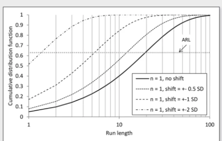
= 0.27% (Minnitt and Pitard, 2008).

Figure 6 shows the RL distribution for a Gaussian sampling distri-bution with shift

d

equal to 0, ± 1 and ± 2 standard deviation, using a risk

a

= 5% and sample size n = 1.

Full sampling distribution and control charts

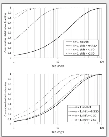
The effect of departure from normality on control charts has led to a number of publications in relation to quality control (Borror et al., 1999), and yet, the effect is not fully recognised by industry. The distribution of run lengths is shown in Figure 7 for the bimodal (b) distribution. The first and most important observation is that the RL distributions are not the same for positive and negative shifts of the mean. This result, which is due to the asymmetry of the sampling distribution, does not appear to have been reported elsewhere as it is not common for asymmetrical sampling distributions to be used in Statistical Process Control.

Figure 8 provides a graphical explanation as to why the RL dis-tributions are not equal for left and right shift of the mean for asym-metrical sampling distributions. From one single sample measure-ment (n = 1), it is apparent that a positive (right) shift will be detected significantly faster than a negative (left) shift of equal magnitude. For an absolute 1% shift of the mean of the bimodal (b) sampling dis-tribution, the type II error

b

for the left shifted distribution is 83.95%

Figure 6. RL distribution for a Gaussian sampling distribution with shift

d

= 0, ± 0.5, ± 1 and ± 2 standard deviation, for

a

= 5% and n = 1. Average run lengths (ARL) are read at the probability 0.63.

(7)

Issue 5 2015

98 www.impublications.com/wcsb7

TOS

f o r u m

versus 14.83% only for the right shifted distribution, as highlighted by the shaded areas in Figure 8.

At any rate, whether left or right shifts occur, the RL distributions for the bimodal (b) sampling distribution are all different from those of the normal distribution for shifts of the same magnitude.

It can be concluded that assuming normality in setting up and applying control charts for quality control will yield erroneous deci-sion making for non-Gaussian sampling distributions. Even though the above analysis was carried out for Shewhart X-bar charts only for the sake of conciseness and clarity, the same conclusions are expected to apply to any type of control charts.

Conclusions

Lyman (2014) has shown that it is now possible to estimate the actual full sampling distribution from sampling data, as opposed to estimating the sampling variance and assuming a Gaussian sam-pling distribution. The aim of this paper was to assess the benefit of using the actual full sampling distribution for some of the impor-tant uses to which sampling results are put, namely production control, quality assurance and quality control. Through a number of illustrative examples, it was demonstrated that the actual sam-pling distribution should be used in order to apply samsam-pling data to their full potential in production control, quality assurance and quality control. A corollary to that statement is that using sampling variance under the assumption of normality of the sampling distri-bution could yield erroneous analyses, which could lead to wrong decision-making related to Quality Assurance and Quality Control (QAQC).

■For production control during the making of a lot, it was found that knowledge of the full sampling distribution is not necessary for quantifying the precision of the final lot assay, provided a suf-ficient number of samples are taken during the constitution of the lot. However, knowledge of the actual sampling distribution is imperative if a few samples only are used to quantify the as-say of a lot. Since different sampling distributions yield different confidence intervals at the beginning of the making of the lot, us-ing the full samplus-ing distribution is deemed necessary for grade control optimization during production of a commercial lot.

■Assuming normality of the sampling distribution for quality assur-ance can be to the advantage of the seller or the buyer, however there is no way to know without knowledge of the actual pling distribution; hence it is necessary to use the actual sam-pling distribution for quality assurance. These conclusions were obtained by studying the effect of sampling distribution on the OC curve, one key decision-making tool in quality assurance. It was further observed that the greater the departure from normal-ity, the more important it is to use the actual sampling distribution for accepting conforming and rejecting nonconforming lots.

■For quality control, the effect of using the actual sampling distribution on the RL distribution for Shewhart X-bar charts was investigated. It was found that the RL distribution, which encapsulates the efficiency of control charts for detecting shifts in quality in any production process, was highly sensitive to the nature of the full sampling distribution. The conclusion is that the actual sampling distribution must be used for application of con-trol charts in quality concon-trol. Interestingly, it was observed that asymmetrical sampling distributions, which are likely to occur with particulates, yield RL distributions that are sensitive to the sign of the shift.

References

1. Lyman, G., Determination of the complete sampling distribution for a particulate material, in Proceedings of Sampling 2014, 29-30 July 2014, Perth, Australia, AusIMM, Publications series No 5/2014, pp. 17-24 (2014).

2. Lyman, G., “Complete sampling distribution for primary sampling, sam-ple preparation and analysis”, in Proceedings of the 7th International

Conference on Sampling and Blending, Ed by K.H. Esbensen and C.

Wagner, TOS forum Issue 5, 87–91 (2015). doi: 10.1255/tosf.44

Figure 8. Full sampling distributions – bimodal (b) – with mean assay 41% (shift = –1%), 42% (no shift) and 43% (shift = + 1%) from left to right. The vertical lines show the lower (LCL) and upper (UCL) control limits at the 95% confidence level.

Figure 7. RL distribution for the bimodal (b) sampling distribution, for

a

= 5% and n = 1. The upper Figure is for positive shifts of the mean, and the lower Figure for negative shifts of the mean.

(8)

Issue 5 2015

99 TOS

f o r u m

www.impublications.com/wcsb7

3. Venter, J.H., A model for the distribution of concentrations of trace ana-lytes in samples from particulate materials, Technometrics, 24(1), pp. 19-27 (1984).

4. Shmueli, G., Practical acceptance sampling – A hands-on guide, 2nd

Edition (2014). ISBN 978-1-463-78904-6.

5. FAO - Food and Agriculture Organization of the United Nations. Myco-toxin Sampling Tool – User Guide, http://www.fstools.org/mycotoxins/, Sections 1.2 and 2.3 (2014).

6. Bourgeois, F.S., and Lyman, G.J., Quantitative estimation of sampling uncertainties for mycotoxins in cereal shipments, Food Additives &

Contaminants: Part A: Chemistry, Analysis, Control, Exposure & Risk Assessment, 29:7, 1141-1156 (2012).

7. Lyman, G. J., Bourgeois, F.S., and Tittlemier, S., Use of OC curves in quality control with an example of sampling for mycotoxins, in

Proceed-ings 5th World Conference on Sampling and Blending (WCSB5),

San-tiago, Chile, 25-28 October 2011, pp. 431-443 (2011).

8. Minnitt, R.C.A. and Pitard, F., Application of variography to the control of species in material process streams: %Fe in an iron ore product, The Journal of the Southern African Institute of Mining and Metallurgy, 108, 109-122.

9. Borror, C.M., Montgomery, D.C., and Runger, G.C., Robustness of the EWMA control chart to non-normality, Journal of Quality Technology, 31, pp. 309-316 (1999).

Appendix

Skew-normal distribution

The skew-normal distribution is a useful distribution for simulating a skewed Gaussian looking distribution. It is a three parameter distri-bution whose density distridistri-bution function is defined by:

4. Shmueli, G., Practical acceptance sampling – A hands-on guide, 2nd_{Edition (2014). ISBN 978-1-463-78904-6.}

5. FAO - Food and Agriculture Organization of the United Nations. Mycotoxin Sampling Tool – User Guide, http://www.fstools.org/mycotoxins/, Sections 1.2 and 2.3 (2014).

6. Bourgeois, F.S., and Lyman, G.J., Quantitative estimation of sampling uncertainties for mycotoxins in cereal shipments, Food Additives & Contaminants: Part A: Chemistry, Analysis, Control, Exposure & Risk Assessment, 29:7, 1141-1156 (2012).

7. Lyman, G. J., Bourgeois, F.S., and Tittlemier, S., Use of OC curves in quality control with an example of sampling for mycotoxins, in Proceedings 5th_{World Conference on Sampling and Blending (WCSB5), Santiago, Chile, 25-28 October 2011, pp. 431-443}

(2011).

Appendix

Skew-normal distribution

The skew-normal distribution is a useful distribution for simulating a skewed Gaussian looking distribution. It is a three parameter distribution whose density distribution function is defined by:<Eq D>

( ) 2 x x f x f x f a x w w w æ ö æ - ö_{÷ ç} æ _{- ÷}ö_÷ ç ç _÷ = èçç ÷÷÷ø èççç çèç ø÷÷÷÷÷ø

where f is the density distribution function of the standard normal distribution. The parameter a defines the skewness of the distribu-tion. The mean and variance of the distribution are:<Eq E>

2 2 2 2 2_where 1 2 1 a m x wd d p a d s w p = + = + æ _ö÷ ç _÷ = ç_ç- _÷_÷ çè ø

The skew-normal distribution, with set skewness parameter a, is set to any true (unknown) mean m and variance s2_{of the lot using}

the following parameters: <Eq F>

2 2 2 2 2 1 2 2 1 s w d p s x m d p d p =_æ ö÷ ç_- _÷ ç ÷ ç ÷ çè ø = -_æ ö÷ ç_- _÷ ç ÷ ç ÷ çè ø

Figure 9 shows the flexibility of the skew-normal distribution, which provides a mean for simulating left and right skewed distribu-tions.

Figure 10 gives an example of shifted skew-normal distributions with a shift in mean value only, as used in the section about the OC-curve. It suffices to shift the parameter z to shift the mean of the skew-normal distribution without changing its shape.

Bimodal distribution

The bimodal distribution used in this work, with mean m and variance s2_{, is a mixture of two Gaussian random variables as shown in}

Figure 11. It is a five parameter distribution whose parameters are defined as: <Eq G>

( ) ( 1 1) ( )( 2 2) 1 2 2 2 2 2 2 1 1 where i i m am a m s a s d a s d d m m = + -= + + - + =

-

The parameters m1 and m2 are the modes of the distribution, whereas the variances s1 2_{and s}

2

2_{define the spread of both peaks. The}

parameter a is a weighting factor for the mixture of distributions. Figure 12 gives an example of shifted bimodal distributions with a shift in mean value only, as used in the OC-curve section of the paper. It suffices to shift the parameters m1 and m2 by the same amount

in order to shift the mean of the bimodal distribution without changing its shape.

Figure 1. Four distributions with identical mean m = 42% and standard deviation  = 0.5%. The skew-normal distribution has parameters a = –8, x = 42.65%, w = 0.82%. The bimodal (a) and (b) distributions have parameters a = 0.2, m₁ = 41.20%,

s₁ = 0.20%, m₂ = 42.20%, s₂ = 0.32% and a = 0.17, m₁ = 41.00%, s₁ = 0.40%, m₂ = 42.20%, s₂ = 0.15% respectively (see appendix for details).

Figure 2. Evolution of grade during the making of a commercial lot, with the sampling distributions from Figure 1. Figure 3. Example of OC curve for a Gaussian sampling distribution FX = À(42%, 0.5%), with LAQL = 41%.

Figure 4. Illustration of the effect of sampling precision (values are 1 standard deviation s of the full sampling distribution) on

where

f

is the density distribution function of the standard normal distribution. The parameter

a

defines the skewness of the distribu-tion. The mean and variance of the distribution are:

4. Shmueli, G., Practical acceptance sampling – A hands-on guide, 2nd_{Edition (2014). ISBN 978-1-463-78904-6.}

5. FAO - Food and Agriculture Organization of the United Nations. Mycotoxin Sampling Tool – User Guide, http://www.fstools.org/mycotoxins/, Sections 1.2 and 2.3 (2014).

6. Bourgeois, F.S., and Lyman, G.J., Quantitative estimation of sampling uncertainties for mycotoxins in cereal shipments, Food Additives & Contaminants: Part A: Chemistry, Analysis, Control, Exposure & Risk Assessment, 29:7, 1141-1156 (2012).

(2011).

Appendix

Skew-normal distribution

( ) 2 x x f x f x f a x w w w æ ö æ - ö_{÷ ç} æ _{- ÷}ö_÷ ç ç ÷ = èçç ÷÷÷ø èççç çèç ø÷÷÷÷÷ø

2 2 2 2 2_where 1 2 1 a m x wd d p a d s w p = + = + æ _ö÷ ç _÷ = çç_çè- ÷÷_ø

2 2 2 2 2 1 2 2 1 s w d p s x m d p d p =_æ ö÷ ç_- _÷ ç ÷ ç ÷ çè ø = -_æ ö÷ ç_- _÷ ç ÷ ç ÷ çè ø

Bimodal distribution

( ) (1 1) ( )( 2 2) 1 2 2 2 2 2 2 1 1 where _i _i m am a m s a s d a s d d m m = + -= + + - + =

-

2

Figure 1. Four distributions with identical mean m = 42% and standard deviation  = 0.5%. The skew-normal distribution has parameters a = –8, x = 42.65%, w = 0.82%. The bimodal (a) and (b) distributions have parameters a = 0.2, m1 = 41.20%,

s1 = 0.20%, m2 = 42.20%, s2 = 0.32% and a = 0.17, m1 = 41.00%, s1 = 0.40%, m2 = 42.20%, s2 = 0.15% respectively (see

appendix for details).

The skew-normal distribution, with set skewness parameter

a

, is set to any true (unknown) mean

m

and variance

s

2_{of the lot using}

the following parameters:

Additives & Contaminants: Part A: Chemistry, Analysis, Control, Exposure & Risk Assessment, 29:7, 1141-1156 (2012).

(2011).

Appendix

Skew-normal distribution

( ) 2 x x f x f x f a x w w w æ ö æ - ö_{÷ ç} æ _{- ÷}ö_÷ ç ç ÷ = èçç ÷÷÷ø èççç çèç ø÷÷÷÷÷ø

2 2 2 2 2_where 1 2 1 a m x wd d p a d s w p = + = + æ _ö÷ ç _÷ = çç_çè- ÷÷_ø

2 2 2 2 2 1 2 2 1 s w d p s x m d p d p =_æ ö÷ ç_- _÷ ç ÷ ç ÷ çè ø = -_æ ö÷ ç- ÷ ç ÷ ç ÷ çè ø

Bimodal distribution

( ) ( 1 1) ( )( 2 2) 1 2 2 2 2 2 2 1 1 where _i _i m am a m s a s d a s d d m m = + -= + + - + =

-

2

Figure 1. Four distributions with identical mean m = 42% and standard deviation  = 0.5%. The skew-normal distribution has parameters a = –8, x = 42.65%, w = 0.82%. The bimodal (a) and (b) distributions have parameters a = 0.2, m1 = 41.20%,

s1 = 0.20%, m2 = 42.20%, s2 = 0.32% and a = 0.17, m1 = 41.00%, s1 = 0.40%, m2 = 42.20%, s2 = 0.15% respectively (see

appendix for details).

Figure 10 gives an example of shifted skew-normal distributions with a shift in mean value only, as used in the section about the OC-curve. It suffices to shift the parameter

z

to shift the mean of the skew-normal distribution without changing its shape.

Figure 9. Examples of skew-normal distributions with mean

m

s

= 0.5%. A negative skewness parameter

a

yields a left-skewed distribution, whereas a positive parameter yields a right-skewed distribution.

a

= 0 yields the normal distribution.

Figure 10. Examples of skew-normal distributions with variable mean and standard deviation

s

= 0.5%, as used in the OC-curve section. The parameters used are:

the steepness of the OC curve. The OC curves are calculated for FX = À(42%, s%) with LAQL = 41%.

Figure 6. RL distribution for a Gaussian sampling distribution with shift d = 0, ±0.5, ±1 and ±2 standard deviation, for a = 5%

and n = 1. Average run lengths (ARL) are read at the probability 0.63.

Figure 7. RL distribution for the bimodal (b) sampling distribution, for a = 5% and n = 1. The upper figure is for positive shifts of

the mean, and the lower figure for negative shifts of the mean.

Figure 8. Full sampling distributions – bimodal (b) – with mean assay 41% (shift = –1%), 42% (no shift) and 43% (shift = +1%) from left to right. The vertical lines show the lower (LCL) and upper (UCL) control limits at the 95% confidence level.

Figure 9. Examples of skew-normal distributions with mean m = 42% and standard deviation s = 0.5%. A negative skewness

parameter a yields a left-skewed distribution, whereas a positive parameter yields a right-skewed distribution. a = 0 yields the

normal distribution.

Figure 10. Examples of skew-normal distributions with variable mean and standard deviation s = 0.5%, as used in the

OC-curve section. The parameters used are: <Eq G>

   = 41%, = 0.5% = -8, = 41.65%, = 0.82% = 42%, = 0.5% = -8, = 42.65%, = 0.82% = 43%, = 0.5% = -8, = 43.65%, = 0.82% m s a x w m s a x w m s a x w

Figure 11. Examples of bimodal distributions with mean m = 42% and standard deviation s = 0.5%.

Figure 12. Examples of bimodal distributions with variable mean and standard deviation s = 0.5%, as used in the OC-curve

section. The values of the parameters used are: <Eq H> 2 2 2 1 1 2 1 1 2 1 1 2 = 41%, = 0.5% = 0.4, = 40.00%, = 0.40%, = 41.20%, = 0.15% = 42%, = 0.5% = 0.4, = 41.00%, = 0.40%, = 42.20%, = 0.15% = 43%, = 0.5% = 0.4, = 42.00%, = 0.40%, = 43.20%, = 0.15%    m s a m s m s m s a m s m s m s a m s m s

Table 1. Values of acceptance probabilities for lots whose true (unknown) assays are in the range 40% to 42% with all four sampling distributions considered. Shaded columns represent conforming lots (true assay  LAQL), and unshaded columns nonconforming lots.

Sampling dis-tributions from Figure 1

40% 40.5% 41% 41.5% 42%

Normal 2.2750% 15.87% 50.00% 84.13% 97.72%

Skew-normal 0.0007% 14.68% 57.14% 83.92% 95.59%

Bimodal (a) 0.4985% 13.95% 58.71% 80.18% 96.82%

Bimodal (b) 0.0000% 1.87% 76.30% 84.80% 91.50%

Figure 11. Examples of bimodal distributions with mean

m

s

= 0.5%.

(9)

Issue 5 2015

100 www.impublications.com/wcsb7

TOS

f o r u m

Bimodal distribution

The bimodal distribution used in this work, with mean

m

and vari-ance

s

2_{, is a mixture of two Gaussian random variables as shown}

in Figure 11. It is a five parameter distribution whose parameters are defined as:

(

)

(

1 1

)

(

)

(

2 2

)

1 2 2 2 2 2 2 1 1 where i i m am a m s a s d a s d d m m = + -= + + - + = -

The parameters

m

1 and

m

2 are the modes of the distribution,

whereas the variances

s

1 2_and

_s

2

2_{define the spread of both peaks.}

The parameter

a

is a weighting factor for the mixture of distribu-tions. Figure 12 gives an example of shifted bimodal distributions with a shift in mean value only, as used in the OC-curve section of the paper. It suffices to shift the parameters

m

1 and

m

2 by the same

amount in order to shift the mean of the bimodal distribution without changing its shape.

Figure 12. Examples of bimodal distributions with variable mean and standard deviation

s

= 0.5%, as used in the OC-curve section. The values of the parameters used are:

the steepness of the OC curve. The OC curves are calculated for F_X = À(42%, s%) with LAQL = 41%.

Figure 6. RL distribution for a Gaussian sampling distribution with shift d = 0, ±0.5, ±1 and ±2 standard deviation, for a = 5%

and n = 1. Average run lengths (ARL) are read at the probability 0.63.

Figure 7. RL distribution for the bimodal (b) sampling distribution, for a = 5% and n = 1. The upper figure is for positive shifts of

the mean, and the lower figure for negative shifts of the mean.

Figure 8. Full sampling distributions – bimodal (b) – with mean assay 41% (shift = –1%), 42% (no shift) and 43% (shift = +1%) from left to right. The vertical lines show the lower (LCL) and upper (UCL) control limits at the 95% confidence level.

Figure 9. Examples of skew-normal distributions with mean m = 42% and standard deviation s = 0.5%. A negative skewness

parameter a yields a left-skewed distribution, whereas a positive parameter yields a right-skewed distribution. a = 0 yields the

normal distribution.

Figure 10. Examples of skew-normal distributions with variable mean and standard deviation s = 0.5%, as used in the

OC-curve section. The parameters used are: <Eq G>

   = 41%, = 0.5% = -8, = 41.65%, = 0.82% = 42%, = 0.5% = -8, = 42.65%, = 0.82% = 43%, = 0.5% = -8, = 43.65%, = 0.82% m s a x w m s a x w m s a x w

Figure 11. Examples of bimodal distributions with mean m = 42% and standard deviation s = 0.5%.

Figure 12. Examples of bimodal distributions with variable mean and standard deviation s = 0.5%, as used in the OC-curve

section. The values of the parameters used are: <Eq H> 2 2 2 1 1 2 1 1 2 1 1 2 = 41%, = 0.5% = 0.4, = 40.00%, = 0.40%, = 41.20%, = 0.15% = 42%, = 0.5% = 0.4, = 41.00%, = 0.40%, = 42.20%, = 0.15% = 43%, = 0.5% = 0.4, = 42.00%, = 0.40%, = 43.20%, = 0.15%    m s a m s m s m s a m s m s m s a m s m s

Table 1. Values of acceptance probabilities for lots whose true (unknown) assays are in the range 40% to 42% with all four sampling distributions considered. Shaded columns represent conforming lots (true assay  LAQL), and unshaded columns nonconforming lots.

Sampling dis-tributions from Figure 1

40% 40.5% 41% 41.5% 42%

Normal 2.2750% 15.87% 50.00% 84.13% 97.72%

Skew-normal 0.0007% 14.68% 57.14% 83.92% 95.59%

Bimodal (a) 0.4985% 13.95% 58.71% 80.18% 96.82%