Large eddy simulation of thermal cracking in petroleum industry

(1)

En vue de l'obtention du

DOCTORAT DE L'UNIVERSITÉ DE TOULOUSE

Délivré par :

Institut National Polytechnique de Toulouse (INP Toulouse) Discipline ou spécialité :

Energétique et Transferts

Présentée et soutenue par :

Mme MANQI ZHU le mardi 5 mai 2015

Titre :

Unité de recherche : Ecole doctorale :

SIMULATION AUX GRANDES ECHELLES DU CRAQUAGE THERMIQUE

DANS L'INDUSTRIE PETROCHIMIQUE

Mécanique, Energétique, Génie civil, Procédés (MEGeP)

Centre Européen de Recherche et Formation Avancées en Calcul Scientifique (CERFACS) Directeur(s) de Thèse :

MME BENEDICTE CUENOT MME ELEONORE RIBER

Rapporteurs :

M. FRANCK NICOUD, UNIVERSITE MONTPELLIER 2 M. KEVIN VON GEEM, UNIVERSITE DE GENT

Membre(s) du jury :

1 M. LAURENT JOLY, ISAE TOULOUSE, Président

2 M. ANDRÉ NICOLLE, IFPEN, Membre

2 M. DAVID J. BROWN, TOTAL PETROCHEMICALS, Membre

2 Mme BENEDICTE CUENOT, CERFACS, Membre

(2)

(3)

(4)

Acknowledgements

I would like to express the deepest appreciation to my supervisors Bénédicte Cuenot and Eléonore Riber for their supervision of my PhD thesis during more than three years at CERFACS, for their support, advice, valuable comments and suggestions. They encourage me a lot, stay by my side giving me care and shelter in doing this research, share their knowledge and idea, and help in the analysis of results and in the simulations. They also give invaluable suggestions to my presentations and an endless help to finish this manuscript. Especially near the end of my thesis, the warm and serious manner of my supervisors gives me lots of encouragement, confidence and console. Without their guidance and persistent help which benefited me much, this dissertation would not have been possible.

I also want to give my grateful thanks to Thierry Poinsot, who also play an important role in this project, giving me this opportunity to work on this topic at CERFACS, and share many helpful ideas and discussions during my thesis.

I place on record, my sense of gratitude to Philippe Ricoux from TOTAL. S.A for the financial support to my PhD project, the valuable discussions and warm welcome to the meetings organized by TOTAL. In addition, a thank you to David Brown and Dominique Viennet for providing necessary data and documents, and their time for discussing in the regular meeting two times per year and for checking this manuscript.

It also gives me great pleasure in acknowledging the cooperation and support from Kevin Van Geem and his student David Van Cauwenberge at Gent University, who have provided very useful information and chemical schema used in my thesis.

I would like to thank Julien Bodart for his time and effort in conducting simulations using CharLesX_{, making possible the comparison between my results and his, which becomes one}

section of my thesis. It is a good experience working with him during the summer in Stanford and I really appreciate his helpful discussions.

I am also very grateful to Franck Nicoud who gives me lot of advices and patience on my work concerning the numerical schemes.

It’s my privilege to thank the seniors, engineers at CERFACS: Olivier Vermorel, Gabriel Staffelbach, Jérôme Dombard, Laurent Gicquel, for their competent experience and providing me necessary help and valuable suggestions during my research pursuit.

I am indebted to my friendly colleagues who support me much on my life and work at CERFACS: Matthias Kraushaar, Patricia Sierra-Sanchez, Benedetta Giulia Franzelli, An-toine Dauptain, Geoffroy Chaussonnet who I have meet during my internships at CERFACS in 2009 and 2010, give me genuine help and warm welcome in the beginning of thesis; my co-office Lucas Esclapez for his consistent help of any problems and helpful discussions on my thesis topic; Antony Misdariis, Corentin Lapeyre, Michaël Bauerheim, Raphael Mari,

(5)

Dorian Lahbib for their valuable advices for time to time and the joyful lunch time with them; Gaofeng Wang, Pierre Quillatre, R´emy Fransen, Cl´ement Durochat, Adrien Bon-homme and Thomas Livebardon, for providing helpful information and help analyzing the results; Thomas Jaravel and Anne Felden for their help and suggestions about the use of Cantera. I am also very happy to be colleagues with Luis Miguel Segui Troth, Jérôme de Laborderie, David Barre, Abdulla Ghani, Franchine Ni, Sandrine Berger, Francis Shum-Kivan, César Becerril, Damien Paulhiac. I could not list all but they all make me a beautiful memeory.

I’d like also thank Isabelle D’Ast, G´erard Dejean, Fabrice Fleury, Patrick Laporte and other CSG people for their helpful technical support.

Another thank you to Séverine Toulouse for her providing the necessary reading materials needed in my accomplishment of this study; Marie Labadens, Nicole Boutet for taking care of me all the time, and for the help in printing this manuscript; Mich`ele Campassens, Chantal Nasri, Lydia Otero and other ADM people for their help and amity during my life at CERFACS.

Finally I remain indebted to my friends Yi Gao, Le Cui, Yali Meng for their help preparing the day of my defense. Thanks to all of my friends (Wenjie, Qingxiao, Yue, Yihui, Xiaoxuan, Long...) and my parents for their love, moral support and remarkable encouragement.

I would like to thank all the people helping me, encouraging me, taking care of me during my whole PhD thesis, where ever they are, where ever I am.

(6)

To improve the efficiency of thermal-cracking processes, and to reduce the coking phenomena due to high wall temperature, the use of ribbed tubes is an interesting technique as it allows better mixing and heat transfer. However it also induces significant increase in pressure loss. The complexity of the turbulent flow, the chemical system, and the chemistry-turbulence interaction makes it difficult to estimate a priori the real loss of ribbed tubes in terms of selectivity. Experiments combining turbulence, heat transfer and chemistry are very rare in laboratories and too costly at the industrial scale. In this work, Wall-Resolved Large Eddy Simulation (WRLES) is used to study non-reacting and reacting flows in both smooth and ribbed tubes, to show the impact of the ribs on turbulence and chemistry. Simulations were performed with the code AVBP, which solves the compressible Navier-Stokes equations for turbulent flows, using reduced chemistry scheme of ethane and butane cracking for reacting cases.

Special effort was devoted to the wall flow, which is analyzed in detail and compared for both geometries, providing useful information for further development of roughness-type wall models. The impact of grid resolution and numerical scheme is also discussed, to find the best trade-off between computational cost and accuracy for industrial application. Results investigate and analyze the turbulent flow structures, as well as the effect of heat transfer efficiency and mixing on the chemical process in both smooth and ribbed tubes. Pressure loss, heat transfer and chemical conversion are finally compared.

Keywords: Large Eddy Simulation, turbulent reacting flow, roughness, helically ribbed tubes, heat transfer, thermal cracking process

(7)

R´

esum´

e

Pour améliorer l’efficacité des procédés thermiques de craquages et réduire les phénomènes de cokage liés à la température de paroi trop élevée, l’utilisation de tubes nervurés est une technique potentiellement car elle permet d’améliorer le mélange et d’augmenter les transferts de chaleur. Cependant, la perte de charge est significativement augmentée. En raison de la complexité de l’écoulement turbulent, du système chimique et du couplage turbulence-chimie, il est difficile d’estimer a priori la perte réelle en termes de sélectivité des tubes nervurés. Les expériences représentatives de laboratoire combinant turbulence, transferts de chaleur et chimie sont très rares et trop coûteuses à l’échelle industrielle. Dans ce travail, l’approche simulation aux grandes échelles résolue à la paroi (WRLES) est utilisée pour ´

etudier écoulement non-réactif puis réactif dans des tubes à la fois lisses et nervurés, pour quantifier leur impact sur la turbulence et sur la chimie. Le code AVBP, qui résout les ´

equations de Navier-Stokes compressibles pour les écoulements turbulents, est utilisé avec des schémas chimique réduites du craquage de l’éthane puis du butane.

L’écoulement à la paroi est analysé en détail et comparé pour les deux géométries, four-nissant des informations utiles pour le développement ultérieur de modèles de parois pour ce type de rugosité. L’impact de la résolution du maillage et du schéma numérique est ´

egalement discuté, pour trouver le meilleur compromis entre coût et précision de calcul pour une application industrielle. L’impact des structures d’écoulement turbulent ainsi que leurs effets sur le transfert thermique et le mélange sur les réactions chimique sont étudiés à la fois pour les tubes lisses et les tubes nervurés. Perte de pression, transfert de chaleur et conversion chimique sont finalement comparés.

Mots clés: Simulation aux grandes échelles, écoulement turbulent réactif, rugosité, tubes en hélices nervurées, transfert thermique, craquage

(8)

List of Figures

1.1.1 Total Refining & Chemicals, Usine de Gonfreville l’Orcher. source: TOTAL 2

1.1.2 Some of the petrochemical products in daily life [2] . . . 3

1.1.3 Typical fired heater. . . 4

1.2.1 Cracking tubes (vertical, in two planes) in the radiation zone of the pyrolysis furnace. Source: Total Petrochemicals . . . 5

1.2.2 Twisted tape inserts [9] . . . 5

1.2.3 Illustration of the “sand-grain” roughness. . . 6

1.2.4 Dimpled tube [13]: 3D roughness . . . 6

1.2.5 Different types of 2D roughness . . . 6

1.3.1 Helically ribbed steam cracking tube MERT [27] . . . 7

1.3.2 Heat transfer (a) and pressure loss (b) measurements in the normal MERT tube compared with a smooth tube [24] . . . 7

2.1.1 RANS, LES and DNS in the turbulent energy spectrum [51]. . . 15

2.1.2 Boundary layer, showing transition from laminar to turbulent condition. Source: courtesy of Symscape [68]. . . 18

2.1.3 An illustration of the 2D domain of wall flow. . . 19

2.1.4 Wall flow structure in a fully developed turbulent flow in a pipe [77] . . . . 21

2.1.5 Mean temperature profiles in wall units for turbulent pipe flows: Pr depen-dence effect [43]. . . 22

2.1.6 Typical streamwise velocity profile of fully developed turbulent pipe flow [77]. 23 2.1.7 Various power-law velocity profiles for different exponents n, comparing with the fully developed laminar flow [77] . . . 23

2.1.8 Dimensionless RMS of velocity fluctuations u0 +_x,rms, u0 +_θ,rms and u0 +_r,rms versus the dimensionless radius r/R for fully developed turbulent pipe flow [34] . . 24

2.1.9 Dimensionless temperature fluctuation of turbulent pipe flows: Pr depen-dence effect [43]. . . 25

2.2.1 Moody diagram - friction factor vs Reynolds number [32]. . . . 29

2.3.1 Illustration of turbulent flow structure with the separation and reattachment mechanisms in a ribbed channel [103]. . . 33

2.3.2 Recirculation flow patterns over transverse ribs as a function of rib pitch in a ribbed channel [14, 105]. . . 33

2.3.3 Numerotation of successive locations between two ribs A and B, with dis-tances expressed in rib height e unit. . . . 34

(15)

LIST OF FIGURES

2.3.4 Mean streamwise velocity field with the streamlines in ribbed channel where

p/e = 8 [99]. . . . 35

2.3.5 Mean normalized streamwise velocity profiles at different locations in a ribbed channel where p/e = 10 (experimental results: symbols) [95]. LES results are also plotted with lines [112]. . . 35

2.3.6 Mean streamwise velocity profiles over smooth and ribbed walls, normalized by the mixed outer velocity [99]. . . 36

2.3.7 Mean streamwise velocity profiles in wall units for two locations II and IV be-tween ribs (black symbols), comparing with the experimental data of smooth wall (white symbols) [115], and DNS results are also plotted in lines [111]. . 36

2.3.8 Profiles of the mean velocity fluctuations u0_rms and v0_rms normalized by the bulk velocity Ub, at different locations in a ribbed channel where p/e = 10 (experimental results: symbols) [95]. LES results are also plotted in lines for two locations [112]. . . 37

2.3.9 Streamwise Reynolds normal stress over the smooth and ribbed walls [99]. . 38

2.3.10 Dimensionless temperature profiles in ribbed channel (p/e = 7.2) [101]. . . 39

2.3.11 Distribution of local friction factor over ribbed wall (p/e = 8) [97]. . . . 39

2.3.12 Distribution of Nusselt number over ribbed wall (p/e = 7.2) [101]. . . . 40

2.4.1 Geometrical parameters range of some investigators. . . 42

2.4.2 Relation between Rf and e+ [12]. . . 42

2.4.3 Friction correlation for transversal ribbed tubes by Webb et al. [14]. . . 43

2.4.4 Multi-started and single-started helically ribbed tube. . . 44

2.4.5 Friction correlations for multi-started helically ribbed tubes having p/e = 15 with different helix angles [15]. . . 44

2.4.6 Friction correlation for flow in helical-wire-coil-inserted tubes by Sethumad-havan & Rao [17]. . . 45

2.4.7 Global friction factor correlations versus Reynolds number according to pub-lished experimental works for the ribbed tube considered in the present work 47 2.4.8 Heat transfer correlation for transversal ribbed tubes by Webb et al. [14] . 48 2.4.9 Heat transfer correlation data for helically ribbed tubes by Gee et al. [15]. . 49

2.4.10 Global Nusselt number correlations versus Reynolds number according to published experimental works for the ribbed tube of present work . . . 50

2.4.11 St/Sts vs. e+ by Gee et al. [15]. . . 51

2.4.12 Efficiency index η vs. e+ _{by Gee et al. [15]. . . .} ₅₁

2.4.13 Performance evaluation criterion R3 vs. severity index φ for Prandtl 6 and 60 [16]. . . 52

2.4.14 Sketch of the contact angle β of rib. . . . 53

2.4.15 Test cases of Chandra et al. [128]: a) cross section of test channel, b) ribbed wall geometry, c) cases with various rib profiles . . . 53

2.5.1 Distribution of local pressure coefficient over ribbed wall (p/e = 10) [150]. . 56

3.1.1 Configuration of helically ribbed tube with 10 periodic patterns. . . 63

3.2.1 Meshes Y1 for smooth (S51) and ribbed (R51) tubes. . . 64

(16)

3.4.1 Configurations of helicoidally ribbed tubes with 1, 3 or 5 periodic patterns. 68 3.4.2 Friction factor vs Reynolds number of helically ribbed tube R51 with 1, 3

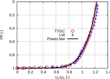
or 5 periodic patterns. . . 69 3.5.1 Mean axial velocity profile in smooth tube S51: cases S51 Y1 TT (circles)

and S51 Y1 LW (crosses), compared to the power law of turbulent pipe flow velocity (solid line). . . 70 3.5.2 RMS of velocity fluctuations u0+_x,rms, u0+_θ,rms and u0+_r,rms in smooth tube S51 on

mesh Y1, compared with existing experiments/DNS data. . . 71 3.5.3 Tube center and 1/4 radius points. . . . 71 3.5.4 Kinetic energy spectrum in both cases S51 Y1 TT and S51 Y1 LW at two

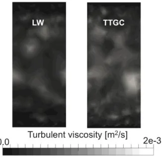
locations. . . 72 3.5.5 Turbulent viscosity on the transverse plane in both cases S51 Y1 TT and

S51 Y1 LW. . . 72 3.5.6 Wall flow in the smooth tube S51 on mesh Y1: WRLES results compared

with the law of the wall and the DNS results from Eggels (1994) [39]. . . . 73 3.5.7 RMS of velocity fluctuations normalized by uτ, u0+x,rms, u

0+

θ,rms and u

0+

r,rms, in

the boundary layer of smooth tube S51 on mesh Y1, compared with DNS data from Wu & Moin (2008) (DNS, Re=44 000) [183]. . . 74 3.6.1 Mean axial velocity profiles of S51 Y1 TT, S51 Y10t TT and S51 Y10t LW 75 3.6.2 Kinetic energy spectrum in the smooth tube S51 with mesh Y10t, compared

to the reference case. . . 76 3.6.3 Turbulent viscosity on the transverse plane of three cases in S51. . . 76 3.6.4 Non-dimensional velocity profile for cases S51 Y10t TT and S51 Y10t LW,

compared to S51 Y1 TT. . . 77 3.6.5 RMS of velocity fluctuations normalized by uτ, u0+x,rms, u

0+

θ,rms and u

0+

r,rms,

in the boundary layer of smooth tube S51 on mesh Y10t, compared to S51 Y1 TT. . . 78 3.7.1 Turbulent flow in the ribbed tube R51 Y1 TT: instantaneous Q-criterion

iso-surface, colored by axial velocity. Black corresponds to recirculating flow. 79 3.7.2 Transverse and axial cut planes in ribbed tube R51. . . 80 3.7.3 Mean axial velocity fields normalized by Ub in transverse planes at three

positions in ribbed tube R51. . . 80 3.7.4 Mean axial velocity field normalized by Ubin the ribbed tube case R51 Y1 TT.

The white lines mark zero axial velocity and the 99% of bulk velocity. Left: transverse cut; Right: half of axial cut, repeated on two periodic patterns. . 81 3.7.5 Mean azimuthal velocity field normalized by Ub in the ribbed tube case

R51 Y1 TT. Left: transverse cut. Right: half of axial cut. . . 81 3.7.6 Mean axial and azimuthal velocity profiles normalized by Ub, at various

locations along the ribbed tube case R51 Y1 TT. . . 82 3.7.7 RMS of the axial fluctuating velocity field u0_rms normalized by Ub in the

ribbed tube case R51 Y1 TT. Left: transverse cut. Right: half of axial cut. 83 3.7.8 Mean pressure coefficient fields in the ribbed tube case R51 Y1 TT. Left:

(17)

LIST OF FIGURES

3.8.1 u+ (normalized by global uτ,g) vs y+ at five locations in the ribbed tube

R51, compared to results in the smooth tube S51. . . 85 3.8.2 RMS of velocity fluctuations normalized by surface averaged uτ: u0+x,rms,

u0+_θ,rms and u0+_r,rms, in the ribbed tube R51 at 5 locations, compared to data in smooth tube S51. . . 86 3.8.3 RMS of velocity fluctuations normalized by Ub in the ribbed tube R51 at 5

locations, compared to smooth tube S51. . . 87 3.8.4 Kinetic energy spectrum in both tubes S51 and R51, with Y1 and TTGC. . 88 3.8.5 Turbulent viscosity on the transverse plane of S51 and R51. . . 89 3.8.6 Friction factors versus Reynolds number in ribbed tube R51 and smooth

tube S51, compared to published experimental works. . . 89 3.8.7 Evolution of the pressure coefficient Cp along the wall surface in both ribbed

(R51 Y1 TT) and smooth (S51 Y1 TT) tubes. . . 90 3.8.8 Evolution of the skin friction coefficient Cf along the wall surface in both

ribbed (R51 Y1 TT) and smooth (S51 Y1 TT) tubes. . . 91 3.9.1 Difference in rib geometry in the configuration R51 for AVBP (A) and

CharLesX _{(B). . . .} ₉₃

3.9.2 Mesh of ribbed tube for LES code CharLesX_{: y}+ _{= 1 with hexahedra (by} Dr. Julien Bodart). . . 93 3.9.3 Mean axial velocity fields normalized by Ub in ribbed tube R51. Left:

R51 Y1 TT using AVBP; Right: R51 Y1h using CharLesX_{. . . .} ₉₄

3.9.4 Mean azimuthal velocity field normalized by Ub in ribbed tube R51. Left:

R51 Y1 TT using AVBP; Right: R51 Y1h using CharLesX_{. . . .} ₉₅

3.9.5 Time-averaged axial velocity profiles (normalized by Ub) in ribbed tube R51

with AVBP and CharLesX. A zoom on the boundary layer is shown in the bottom part of the figure. . . 95 3.9.6 Time-averaged azimuthal velocity profiles normalized by Ub in ribbed tube

R51 with AVBP and CharLesX. A zoom on the boundary layer is shown in the bottom part of the figure. . . 96 3.9.7 RMS of axial fluctuating velocity fields normalized by Ub in ribbed tube

R51. Left: R51 Y1 TT using AVBP; Right: R51 Y1h using CharLesX_. _{. .} ₉₆

3.9.8 Cpfields in ribbed tube R51. Left: R51 Y1 TT using AVBP; Right: R51 Y1h

using CharLesX_{. . . .} ₉₇

3.9.9 Evolution of the pressure coefficient Cp along the wall surface for AVBP and

CharLesX simulations. . . . 98 3.9.10 Evolution of the skin friction coefficient Cf along the wall surface for AVBP

and CharLesX simulations. . . . 98 3.9.11 Dimensionless distance y+ of the closest node to the wall of the mesh used

in the CharLesX _{simulation. . . .} ₉₉

3.10.1 Time-averaged axial velocity fields normalized by Ubin ribbed tube R51.

Up-per: R51 Y1 TT; Bottom left: R51 Y10t TT; Bottom right: R51 Y10tp TT. 100 3.10.2 Time-averaged azimuthal velocity fields normalized by Ub in ribbed tube

(18)

3.10.3 Time-averaged axial velocity profiles normalized by Ub in ribbed tube R51

on the three meshes Y1, Y10t and Y10pt. A zoom on the boundary layer is shown in the bottom part of the figure. . . 102 3.10.4 Time-averaged azimuthal velocity profiles normalized by Ub in ribbed tube

R51 on the three meshes Y1, Y10t and Y10pt. A zoom on the boundary layer is shown in the bottom part of the figure. . . 103 3.10.5 RMS of axial fluctuating velocity fields normalized by Ub in ribbed tube R51.

Upper: R51 Y1 TT; Bottom left: R51 Y10t TT; Bottom right: R51 Y10tp TT.103 3.10.6 Time-averaged pressure coefficient fields in ribbed tube R51 on different

meshes. . . 104 3.10.7 Evolution of the pressure coefficient Cp along the wall surface on the three

meshes Y1, Y10t and Y10pt. . . 104 3.10.8 Evolution of the skin friction coefficient Cf along the wall surface on the

three meshes Y1, Y10t and Y10pt. . . 105 3.11.1 Mean axial velocity fields normalized by Ub in ribbed tube R51. Top left:

R51 Y1 TT; Top right: R51 Y10t TT; Bottom left: R51 Y1 LW; Bottom right: R51 Y10t LW. . . 107 3.11.2 Mean azimuthal velocity fields normalized by Ub in ribbed tube R51. Top

left: R51 Y1 TT; Top right: R51 Y10t TT; Bottom left: R51 Y1 LW; Bot-tom right: R51 Y10t LW. . . 107 3.11.3 Mean axial velocity profiles normalized by Ub in ribbed tube R51, using two

meshes and two numerical schemes. A zoom on the boundary layer is shown in the bottom part of the figure. . . 108 3.11.4 Mean azimuthal velocity profiles normalized by Ub in ribbed tube R51, using

two meshes and two numerical schemes. A zoom on the boundary layer is shown in the bottom part of the figure. . . 109 3.11.5 RMS of axial fluctuating velocity fields normalized by Ub in ribbed tube

R51, using two meshes and two numerical schemes. . . 109 3.11.6 Time-averaged pressure coefficient fields in ribbed tube R51 on different

meshes and with two numerical schemes. . . 110 3.11.7 Evolution of the pressure coefficient Cp along the wall surface of ribbed tube

R51, using two meshes and two numerical schemes. . . 110 3.11.8 Evolution of the skin friction coefficient Cf along the wall surface of ribbed

tube R51, using two meshes and two numerical schemes. . . 111 4.2.1 Temporal evolution of SeV in heated smooth tube HS51 Y1 TT (solid line),

and the initial estimation Sconstant

e V (dashed line). . . 116

4.2.2 Profile of the mean axial velocity Ux normalized by the bulk velocity Ub of

the heated flow in the smooth tube, compared to the isothermal flow. . . . 117 4.2.3 Law of the wall of the heated flow in the smooth tube, compared to the

isothermal flow. . . 117 4.2.4 RMS of velocity fluctuations normalized by uτ, thus u0+x,rms, u

0+

θ,rmsand u

0+

r,rms,

in the boundary layer of the heated flow, together with the isothermal flow, in the smooth tube S51 on mesh Y1. . . 118

(19)

LIST OF FIGURES

4.2.5 Time-averaged non-dimensional temperature Θ profile (circles), compared to the dimensionless velocity Ux/Ub profile (solid line): case HS51 Y1 TT. . 119

4.2.6 Non-dimensional temperature profile Θ+ _{vs y}+_{: HS51 Y1 TT . . . 119} 4.2.7 Dimensionless RMS of temperature fluctuation Θ0+_rms of the heated flow in

the smooth tube on mesh Y1. . . 120 4.3.1 Time-averaged non-dimensional temperature Θ of the heated flow in S51 on

coarse mesh Y10t, compared to the reference case on mesh Y1. . . 122 4.3.2 Dimensionless temperature Θ+ of the heated flow in S51 on coarse mesh

Y10t, compared to the reference case on mesh Y1. . . 122 4.3.3 Normalized RMS of the temperature fluctuation Θ0+_rms of the heated flow in

S51 on coarse mesh Y10t, compared to the reference case on mesh Y1. . . . 123 4.4.1 Normalized axial velocity fields of both isothermal and heated flow in the

ribbed tube R51. . . 124 4.4.2 Normalized azimuthal velocity fields of both isothermal and heated flow in

the ribbed tube R51. . . 124 4.4.3 Normalized axial velocity profiles of both isothermal and heated flows in R51.125 4.4.4 Normalized azimuthal velocity profiles of both heated and isothermal flows

in R51. . . 125 4.4.5 Normalized RMS of the axial velocity fluctuation fields of both isothermal

and heated flows in R51. . . 126 4.4.6 Pressure coefficient fields of both isothermal and heated flows in R51 . . . 126 4.4.7 Evolution of the pressure coefficient Cpalong the wall surface of both

isother-mal and heated flows in R51. . . 127 4.4.8 Evolution of the skin friction coefficient Cf along the wall surface of both

isothermal and heated flows in R51. . . 127 4.4.9 Normalized mean temperature fields of the heated flow in S51 and R51. . . 128 4.4.10 Mean normalized temperature profiles of the heated flow at various locations

in both smooth and ribbed tubes . . . 128 4.4.11 Mean normalized temperature profiles of the heated flow at location 5e in

both smooth and ribbed tubes. . . 129 4.4.12 Dimensionless temperature Θ+_{vs y}+_{of the heated flow at 5 various locations}

in the ribbed tube, compared to the heated smooth tube. . . 130 4.4.13 Dimensionless RMS of temperature fluctuations Θ0 +

rms of the heated flow at

5 various locations in the ribbed tube, and compared to the heated smooth tube. . . 131 4.4.14 Evolution of the Nusselt number Nu along the wall surface of the ribbed

tube, compared to the smooth tube. . . 131 4.5.1 Time-averaged fields of the normalized temperature Θ of the heated flow in

the ribbed tube R51 on meshes Y1/Y10t, with TTGC/LW. . . 133 4.5.2 Time-averaged profiles of the normalized temperature Θ of the heated flow

in the ribbed tube on meshes Y1/Y10t, with TTGC/LW. . . 133 4.5.3 Time-averaged fields of the RMS of the fluctuating temperature Trms of the

(20)

4.5.4 Evolution of the Nusselt number along the wall surface in the heated ribbed tube on meshes Y1/Y10t, with TTGC/LW. . . 134 4.5.5 Global Nusselt number correlations versus Reynolds number of the ribbed

tube R51 simulated by AVBP, compared to the correlation proposed by Vicent et al. (2004) [16] and Garcia et al. (2005) [123], and the Dittus-Boelter correlation for the smooth tube. . . 135 5.2.1 Illustration of a PSR configuration. . . 139 5.2.2 Comparison of temporal evolutions of PSR results of ethane cracking on

varying or fixing the pressure in Senkin. . . 140 5.2.3 Comparison of temporal evolutions of PSR results of ethane cracking with

different initial pressure in Cantera. . . 141 5.2.4 Cases C/S/A-CV-A-T9P1 by Cantera, Senkin and AVBP: inlet temperature

at 973 K and inlet pressure at 1 atm. . . 142 5.2.5 Cases C/S/A-CV-A-T12P1 by Cantera, Senkin and AVBP: inlet

tempera-ture at 1200 K and inlet pressure at 1 atm. . . 143 5.2.6 Cases C/A-CV-A-T9P2 by Cantera, Senkin and AVBP: inlet temperature

at 973 K and inlet pressure at 1 atm/2 atm. . . 143 5.2.7 Illustration of the two zero mixing extreme conditions of ethane chemistry

in tubes. . . 144 5.2.8 Quantities evolution of two ZME lines of ethane cracking process . . . 145 5.3.1 Sketch of the global process of reacting heated ethane flow in smooth/ribbed

tubes. . . 145 5.3.2 A simple tube flow with temperature and pressure variation along the axial

distance. . . 146 5.3.3 Unsteady flow in the periodic configuration: the temperature and pressure

vary with time. . . 146 5.4.1 Three instantaneous axial velocity fields of the heated reacting flow in both

smooth and ribbed tubes. . . 147 5.4.2 Time-averaged axial velocity field of the heated reacting flow in both smooth

and ribbed tubes. . . 148 5.4.3 Three instantaneous temperature fields of the heated reacting flow in both

smooth and ribbed tubes. . . 148 5.4.4 Three instantaneous reaction rate fields of the reaction C2H6 → CH3+ CH3

of the heated reacting flow in both smooth and ribbed tubes. . . 149 5.4.5 Temperature and reaction (C2H6 → CH3+ CH3) rate fields in both smooth

and ribbed tubes: zoom in the near wall region. . . 149 5.4.6 Temporal evolutions of spatially-averaged temperature, mole fraction of the

product C2H4 and the two reactants H2O and C2H6 for ethane cracking in both smooth and ribbed tubes. . . 150 5.4.7 Spatially-averaged reaction rate for C2H6 → CH3 + CH3 in both smooth

(S51) and ribbed (R51) tubes. . . 151 5.4.8 Dimensionless temperature profiles of the instantaneous solution at 80 ms in

(21)

LIST OF FIGURES

5.4.9 Relations between the reaction rate of C2H6 → CH3+ CH3, the temperature and the mass fraction of the reactant C2H6 in both smooth (S51) and ribbed (R51) tubes. . . 152 5.4.10 The tube center where the quantities are investigated. . . 153 5.4.11 Evolution of mass fraction of ethane vs the temperature at the center of

both smooth (S51) and ribbed (R51) tubes. . . 153 5.4.12 Temporal evolution of velocities at the center of both smooth (S51) and

ribbed (R51) tubes: (a) axial velocity; (b) radial velocity; (c) azimuthal velocity. . . 154 5.4.13 Location at 1/4 radius where the quantities are investigated. . . 154 5.4.14 Evolution of mass fraction of ethane vs the temperature at 1/4 radius of

both smooth (S51) and ribbed (R51) tubes. . . 154 5.4.15 Temporal evolution of velocities at 1/4 radius of both smooth (S51) and

ribbed (R51) tubes: (a) axial velocity; (b) radial velocity; (c) azimuthal velocity. . . 155 6.1.1 Temporal evolutions of the pressure, the temperature and the mole fractions

of all the 20 species of the PSR case in Cantera (x-axis is time [s]). . . 161 6.1.2 Temporal evolutions of the pressure, the temperature and the mole fractions

of all the 20 species of the PSR case in Senkin (x-axis is time [s]). . . 163 6.1.3 Influence of the simulate time step ∆t in AVBP on the error on C2H4. . . . 164 6.1.4 Comparison of the temporal evolutions of selected quantities obtained with

Cantera (solid line) and AVBP (dashed line) (∆t = 5×10−9s). . . 165 6.2.1 Configuration of both smooth (S38) and ribbed tube (R38) used for the

industrial application. . . 165 6.2.2 Axial cuts of meshes of both smooth (S38) and ribbed tube (R38). . . 166 6.2.3 Imposed heat flux at the wall: in AVBP (crosses), and from the data

pro-vided by TOTAL (solid line for R38 and dashed line for S38). . . 167 6.2.4 Configuration (a) and stable regime (b) of the 2D non-reacting isothermal

laminar flow through a channel. . . 169 6.2.5 Temporal evolutions of P , T , ρ and Ecin for the 3 options of density source

term, compared to the theoretical results. . . 170 6.2.6 Comparison between option 3 and the theoretical results. . . 170 6.2.7 Temporal evolutions of the spatially-averaged pressure, temperature and

mass density using the 3 options, compared to the theoretical results. . . . 172 6.2.8 Pressure decrease imposed in AVBP (solid line) and the data from TOTAL

(symbols: squares) in both S38 and R38 tubes. . . 173 6.3.1 Preliminary PSR tests at different pressures and temperatures with Cantera:

temporal evolutions of the temperature, pressure, mole fraction of reactants and two mains products. . . 174 6.4.1 Temporal evolutions of the spatially-averaged temperature, pressure, mole

fraction of the two main products and the two reactants for both tubes S38 and R38, compared with the data from TOTAL. The x-axis is “Time [S]”. TOTLAL source: symbols. AVBP results: lines. . . 175

(22)

6.4.2 (a)Temporal evolution of spatially-averaged reaction rate of the reaction C4H10 → 2C2H5; (b)-(c) relations between reaction rate, temperature and mass fraction of C4H10 in both S38 and R38 tubes. . . 176 6.4.3 Instantaneous fields of axial velocity in both S38 and R38 tubes at 1 ms,

10 ms and 40 ms. . . 176 6.4.4 Instantaneous fields of temperature in both S38 and R38 tubes at 1 ms,

10 ms and 40 ms. . . 177 6.4.5 Instantaneous skin temperature distribution at the wall in both S38 and R38

tubes at 10 ms. . . 177 6.4.6 Instantaneous fields of the reaction rate of C4H10→ 2C2H5 in both S38 and

R38 tubes at 1 ms, 10 ms and 40 ms. . . 178 6.4.7 Instantaneous fields of mass fraction of C4H10in both S38 and R38 tubes at

1 ms, 10 ms and 40 ms. . . 178 6.4.8 Instantaneous fields of mass fraction of C3H6 in both S38 and R38 tubes at

1 ms, 10 ms and 40 ms. . . 179 6.4.9 Probability distribution of temperature at 10 ms and 40 ms in both S38 and

R38 tubes. . . 180 6.4.10 Probability distribution of reaction rate for C4H10 → 2C2H5 at 10 ms and

40 ms in both S38 and R38 tubes. . . 180 6.4.11 Contribution of reaction rate for C4H10 → 2C2H5 at 10 ms and 40 ms in both

S38 and R38 tubes. . . 181 A.1.1 Computational domain . . . 199

(23)

(24)

List of Tables

2.1.1 Wall regions and their defining properties [28]. . . 20 2.4.1 Summary of experimental studies of ribbed pipes . . . 41 2.4.2 Constant coefficients of Eq. 2.4.17 proposed by different investigators. . . . 46 3.2.1 Mesh information for all the unstructured meshes for both S51 and R51. . 66 3.3.1 Non-reacting isothermal flow in smooth (S51) and ribbed (R51) tubes: list

of test cases. . . 67 3.5.1 Simulation information of case S51 Y1 TT. . . 69 3.5.2 Effective operating points of cases S51 Y1 TT and S51 Y1 LW. . . 70 3.6.1 Convergence and CPU times of cases S51 Y10t TT and S51 Y10t LW. . . . 74 3.6.2 Operating conditions of the turbulent heated flow in smooth tube S51, using

mesh Y10t and the two numerical schemes TTGC and LW, compared to the reference case S51 Y1 TT. . . 75 3.7.1 Convergence/averaging times and CPU cost of case R51 Y1 TT. . . 78 3.7.2 Operating point for the ribbed tube case R51 Y1 TT. . . 79 3.8.1 Boundary layer thickness at different locations in ribbed tube R51, compared

to the smooth tube S51. . . 84 3.8.2 Dimensionless boundary thickness at different locations in ribbed tube R51,

compared to the smooth tube S51. . . 85 3.8.3 Axial momentum equation balance in both ribbed (R51 Y1 TT) and smooth

(S51 Y1 TT) tubes. . . 91 3.9.1 Operating points for ribbed tubes cases: R51 Y1 TT using AVBP and

R51 Y1h using CharLesX_{. . . .} ₉₃

3.9.2 Convergence and CPU times of case R51 Y1h using CharLesX. . . 94 3.9.3 Axial momentum balance in ribbed tube R51 computed using AVBP and

CharLesX_{. . . .} ₉₈

3.10.1 Convergence and CPU times of cases R51 Y10t TT and R51 Y10pt TT. . . 99 3.10.2 Effective operating points of the ribbed tube simulations on different meshes. 100 3.10.3 Axial momentum balance in ribbed tube R51 on the three meshes Y1, Y10t

and Y10pt, with numerical scheme TTGC. . . 105 3.11.1 Convergence and CPU times of cases R51 Y1 LW and R51 Y10t LW. . . . 106 3.11.2 Effective operating points of the turbulent flow in ribbed tube R51 with LW

scheme on meshes Y1 and Y10t. . . 106 3.11.3 Axial momentum balance in ribbed tube R51, using two meshes and two

(25)

4.1.1 Non-reacting heated flow in smooth (S51) and ribbed (R51) tubes. . . 115 4.2.1 Convergence and CPU times of case HS51 Y1 TT. . . 115 4.2.2 Operating conditions of the turbulent heated flow in the smooth tube,

com-pared with the reference case of the isothermal flow. . . 116 4.3.1 Convergence and CPU times of cases HS51 Y10t TT and HS51 Y10t LW. . 121 4.3.2 Operating conditions of the turbulent heated flow in smooth tube S51, using

mesh Y10t and the two numerical schemes TTGC and LW, compared to the reference case. . . 121 4.4.1 Convergence and CPU times of case HR51 Y1 TT. . . 123 4.4.2 Operating condition of the case HR51 Y1 TT. . . 123 4.5.1 Convergence and CPU times of cases on the mesh Y10t using the two

nu-merical schemes LW and TTGC. . . 132 4.5.2 Operating conditions of the turbulent heated flow in ribbed tubes R51 solved

on the mesh Y10t using the two numerical schemes LW and TTGC, com-pared to the reference case. . . 132 5.2.1 Summary of the PSR test cases of ethane chemistry in Senkin, Cantera and

AVBP. . . 139 5.2.2 PSR tests of the ethane cracking of constant volume/pressure in Senkin. . . 140 5.2.3 PSR tests of the ethane cracking with different initial pressure in Cantera. 140 5.2.4 PSR test cases in Senkin. . . 142 5.2.5 Operating points of the two PSR zero mixing extreme cases. . . 144 6.1.1 The 20 species in the reduced chemical scheme for butane steam cracking

process. . . 158 6.1.2 Initial conditions for PSR cases tested in Cantera and Senkin . . . 159 6.2.1 Mesh information for the unstructured meshes for both S38 and R38. . . . 166 6.2.2 Input parameters and expected results for reacting case using the three

options of density source term. . . 171 6.3.1 Preliminary PSR tests at different pressures and temperatures with Cantera. 174 6.4.1 Probability distribution of reaction rate for C4H10 → 2C2H5 at 10 ms and

40 ms in both S38 and R38 tubes. . . 181 6.4.2 Selectivity of products CH4, C2H4 and C3H6 in both S38 and R38 tubes. . 182 A.3.1 Comparison of the numerical methods in AVBP using two diffusion operators

4∆ and 2∆, together with the analytical resutls for the second derivative terms in PDE. . . 204 E.0.1 Difference in the calculation method of the reverse rate of a given reaction

(26)

Chapter 1 Introduction

1.1 Industrial context

The hydrocarbon processing industry (HPI) and chemical processing industry (CPI) cover all aspects of producing petroleum-based products, including refining of petroleum (a picture of an oil refinery in Fig. 1.1.1), manufacturing of chemical and petrochemicals from petroleum feedstocks, processing of gases, and production of synthetic fuels [1]. These industries take raw materials such as crude oil, natural gas and convert them into usable products, including the gasoline, diesel, fuels and precursor materials for the generation of plastics that go into many products, from clothing to plastic bottles, of our daily life, illustrated on Fig. 1.1.2. A critical factor to all these process is heat as chemical conversion is most efficient in narrow temperature ranges.

A majority of operations in the HPI occur in petroleum refining. The major petroleum refining processes are categorised as: 1) topping (the separation of crude oil), 2) thermal and catalytic cracking, 3) combination/rearrangement of hydrocarbon, 4) treating and 5) specialty product manufacturing [3]. Most of them require a fired heater, as illustrated on Fig. 1.1.3, showing typical exterior and interior structures. In such systems, the flow inside the tubes is heated from outside by the flames of the burners (Fig. 1.1.3b). The major heat transfer processes include radiation and convection: in the radiation section, heat transfer occurs between the flame and process tubes through thermal radiation; in the

(27)

1.1. INDUSTRIAL CONTEXT

Figure 1.1.1: Total Refining & Chemicals, Usine de Gonfreville l’Orcher. source: TOTAL

convection section, hot gases through flowing through a network of tubes generate external convective heat transfer, while the inner tube flow generates internal convective heat transfer, as illustrated in Fig. 1.1.3c.

As one of the major petroleum refining processes, the objective of the cracking process is to produce ethylene C2H4, which is the largest volume building block for many

petro-chemicals. Ethylene can be produced via a myriad of different processes, such as catalytic pyrolysis and hydropyrolysis processes [7], fluidized bed cracking, paraffin dehydrogenation, and oxydehydrogenation [8]. The present work mainly concerns thermal cracking. During the thermal cracking processes, steam-cracking furnaces produce ethylene by heating hydro-carbons such as ethane C2H6, propane C3H8, butane C4H10, naphtha, or gas oils to very high

temperatures in the presence of steam [1], leading to the the thermal decomposition of large molecules into lighter ones. Thermodynamic equilibrium favors the formation of olefins only at high temperature and low pressure. Typical reactor coil outlet temperatures are in the range of 788-885◦C (1061-1158 K), and the pressure is 1.7-2.4 bar. The hydrocarbon partial pressure is lowered by the presence of the dilution steam. Moreover, a high selectivity is achieved by operating with a very short residence time, typically 0.1-0.5 s.

The reactions during cracking processes are highly endothermic. As the residence time in the process tube is very short, a high heat flux is required to maintain the temperature at a level sufficient for the reactions to occur. As a consequence, heat transfer enhancement techniques always play an important role in the exchanger system optimization. Artificial roughness in the inner surface of tubes is one passive method of heat transfer enhancement which, in contrast to active methods, does not require a direct application of external power. Different kinds of artificial roughness are widely used in various industrial applications. In the next section, a classification of the different artificial roughness of tubes is introduced.

(28)

Figure 1.1.2: Some of the petrochemical products in daily life [2]

1.2 Classification of artificial roughness

The cross section of heat exchanger ducts are of different forms, either rectangular (channels) or circular (tubes). As our subject is to study the heat exchanger tubes in a radiation zone of the pyrolysis furnace (i.e. thermal cracking furnace) for the thermal cracking processes (as shown in Fig. 1.2.1), only tubular geometries are discussed.

1.2.1 One/two/three dimensional roughness

Some examples of different families of artificial roughness are introduced in this section. As a big family of the artificial roughness, tubes with twisted tape inserts as illustrated in Fig.1.2.2 and other variations are widely investigated and reviewed in Kumar et al.(2012) [9]. A part from this family, Vicente et al.(2002) [10] presented two types of artificial roughness: 1) two-dimensional roughness includes transverse and helical ribs, helically corrugated and wire coil inserts; 2) three-dimensional roughness includes sand-grain roughness, attached particle roughness, “cross-rifled” roughness and helically dimples. Note that Withers (1980) [11] clas-sified that sand-grain roughness (Fig. 1.2.3) as one-dimensional, because it is characterized by only one parameter: the roughness height “e” according to Nikuradse’s experiments [12]. The 3D helically dimpled roughness is illustrated in Fig. 1.2.4: the height of the roughness e, the pitch between two parallel series of obstacles p and the distance between two neighbor obstacles l compose the three dimensions which influence the behavior of roughness.

In the same way, 2D roughness is described with two parameters, ribs height “e” and pitch “p” as indicated in Fig. 1.2.5, that affect the performance. This study will mainly focus on 2D roughness.

Some illustrations of different 2D roughness types are given in Fig. 1.2.5.

(29)

1.2. CLASSIFICATION OF ARTIFICIAL ROUGHNESS

(a) Exterior. Source from [4].

(b) Interior. Source from [5]. (c) Schematic. Source from [6]

Figure 1.1.3: Typical fired heater.

whereas the wire-coil inserts (Fig.1.2.5d) are wall-attached. Corrugated tubes (Fig.1.2.5c) are characterized by a rough outer surface, contrary to others tubes having a smooth outer surface. The different manufacturing technique may lead to different shapes. Garcia et al. (2012) ( [13]) found that, in the petrochemical industry, the use of mechanically deformed tubes (like the corrugated tubes and dimpled tubes) is not allowed for safety reasons due to the risk of being broken, however, the use of wire coils does not cause any problem.

1.2.2 D-type and K-type

Perry et al.(1969) [19] studied the turbulent boundary layer over a transversally ribbed wall and proposed to distinguish two types of 2D roughness: K-type and D-type, “K” representing the roughness height (in this report “e” will be used as the symbol of the roughness height according to some more recent papers) and “D” the outer scales like boundary-layer thickness, pipe diameter, or channel height. Tani (1987) [20] suggested that, for regularly spaced ribs, a demarcation between K-type and D-type roughness might be made at the pitch to height ratio p/e = 4, where p is the pitch between the roughness elements [21]:

• For D-type, roughness is typified by closely spaced ribs with p/e < 4. The ribs are so closely spaced that stable vortices are set up in the grooves, eddy shedding from the roughness elements into the outer flow is negligible, and the outer flow is relatively undisturbed by the roughness elements. The roughness performance (e.g., its impacts on the friction factor) is independent of the size of roughness.

(30)

Figure 1.2.1: Cracking tubes (vertical, in two planes) in the radiation zone of the pyrolysis furnace. Source: Total Petrochemicals

Figure 1.2.2: Twisted tape inserts [9]

• For K-type roughness, typified by sparsely spaced transverse ribs, with p/e > 4, eddies with length scale of the order of the roughness height are shed from the roughness ele-ments and penetrate into the bulk flow toward the pipe or channel center (or boundary layer edge). The roughness performance depends on the size of the roughness elements. In the present study, only K-type 2D roughness is considered.

1.3 The Mixing Element Radiant Tube technology in

steam-cracking process

In a thermal cracking furnace (Fig. 1.2.1), the cracking tubes are usually 10 meters long. The Reynolds number of the turbulent flow inside the tubes ranges from 104 to 105, and the residence time is typically 0.1-0.5 s. As mentioned in section 1.1, the steam-cracking process is favored at high temperature. At the same time, high tube skin temperature, typically between 1000-1125◦C (1273-1398 K) [1], promots undesired but inevitable formation and deposit of coke (carbon) on the inner wall of the tubes. If the coke layer in the tubes becomes

(31)

1.3. THE MIXING ELEMENT RADIANT TUBE TECHNOLOGY IN STEAM-CRACKING PROCESS

Figure 1.2.3: Illustration of the “sand-grain” roughness.

Figure 1.2.4: Dimpled tube [13]: 3D roughness

(a) Transverse ribs [14] (b) Helical ribs [15]

(c) Helically corrugated [16] (d) Wire coil insert [17]

Figure 1.2.5: Different types of 2D roughness

thicker, the pressure loss and the wall temperature both increase, due to the increase of the wall friction and the reduction of the heat transfer, then the problem gets worse. When either the pressure drop limit or the tube skin temperature limit is reached, the tubes must be decoked. This is a long and uneasy operation, requiring to stop the production, i.e., having a high cost. For this reason, coking phenomena must be avoided as much as possible. For these reasons, heat transfer enhancement techniques is required, which increase the heat transfer efficiency and can reduce the skin temperature. However, note that these techniques often induce increased pressure losses.

Many technologies are developed in order to improve the performance of steam-cracking tubes. Helically ribbed tubes are widely studied and many patents on this technology are submitted. Fig. 1.3.1 shows examples of helically ribbed tubes of the Mixing Element Ra-diant Tube (MERT) family technology [22–26], developed by KUBOTA [27] to be used in tubular pyrolysis furnaces. According to the previous classification, the “normal MERT” [23] (Fig. 1.3.1a) is a 2D roughness type because of the continuous helically ribs on the inner

(32)

(a) Normal MERT (b) Slit-MERT (Below) & X-MERT (Upper)

Figure 1.3.1: Helically ribbed steam cracking tube MERT [27]

surface, while the “slit-MERT” & “X-MERT” (Fig. 1.3.1b) is kind of 3D roughness type as the ribs are non-continuous.

MERT tubes have clear advantages in thermal cracking processes: thanks to enhanced mixing, the wall heat transfer efficiency is improved and the flow in the tube is more ho-mogeneous in both temperature and composition. As a consequence, the temperature of the tube’s skin decreases and coke deposit is reduced [27]. Another result is the improved operating efficiency of the chemical process. Fig. 1.3.2 shows that the heat transfer is around 1.5 times higher than that in a smooth tube in the same condition, while the pressure loss is 3-4 times higher.

(a) Heat transfer vs Reynolds number (b) Pressure loss vs Reynolds number

Figure 1.3.2: Heat transfer (a) and pressure loss (b) measurements in the normal MERT tube compared with a smooth tube [24]

The performance of MERT technology could be optimized by changing the ribs arrange-ment, the ribs height, the ribs pitch, etc. This requires an understanding of the physical phenomena of turbulent flows in ribbed tubes, and to reveal the impact of ribs.

(33)

1.4. AIMS OF THE WORK

1.4 Aims of the work

To achieve heat enhancement while avoiding increased pressure loss and reducing coking phenomena, the main objective of the present work is the understanding of helically ribbed tubes flow dynamics and impact on the chemical process. This requires to face scientific issues as wall flows in tubes, heat transfer in turbulent flows, and interaction of cracking chemistry with turbulence.

Many experimental and numerical research studies have been devoted to the turbulent flow in smooth tubes and wall models have been established, that lead to a correct calculation of both the wall friction and heat flux. The situation is much different for ribbed tubes. Experiments lead to very different results, with no clear conclusions about the nature of the wall flow. Moreover, the experimental instrumentation cost limits the measurements.

For these reasons, numerical simulation appears as an interesting tool to investigate tur-bulent flows in ribbed tubes. Examples of numerical simulations of ribbed tubes, especially of helically ribbed tubes, are much scarce in the literature. In the present work, the turbu-lent flow and heat transfer in a ribbed tube is investigated by use of high-fidelity numerical simulation, with the following objectives:

• to understand the dynamic properties of the turbulent wall flow in ribbed tubes, • to understand heat transfer phenomena of the turbulent wall flow in ribbed tubes, • to understand the impact of ribs on the petrochemical process for the optimization of

the cracking tube,

• to apply numerical simulation to a real industrial system and demonstrate the feasi-bility and added-value of such simulations.

1.5 Outline

• Part I: Chapter 2

The study begins with a literature survey. Experiments are reviewed, showing the dominant geometric parameters of ribbed tubes and their effect on the flow proper-ties. Some semi-experimental correlation formula for calculating the friction factor and Nusselt number (which characterize the heat transfer properties) in the different tubes are also presented.

• Part II: Chapters 3 to 5

To understand the physics of ribbed tube flows, academic cases are first considered in this part. Both smooth and ribbed tubes are simulated in reacting, either non-heated (Chapter 3) or non-heated (Chapter 4) conditions. Special effort is devoted to the wall flow, which is analyzed in detail and compared for both geometries. The impact of grid resolution and numerical scheme is also discussed, to find the best trade-off between computational cost and accuracy for the industrial application.

(34)

process, which is of high interest to the petrochemical industry, is reproduced and analyzed.

• Part III: Chapter 6

In this third part, the methodology developed in Part II is applied to evaluate the efficiency in terms of chemical conversion of a real industrial case, which constitutes the final objective of the work. Both smooth and ribbed tubes with inner diameter of 38 mm, are simulated using the real heat flux and pressure drop applied in the industrial process. The flow is a mixture of butane C4H10and steam (H2O) producing

ethylene.

• Part IV: Chapter 7

(35)

(36)

Chapter 2 Turbulent flows in smooth and rough

tubes

Most flows in nature, in daily life and in industry are turbulent. In real life, and in contrast to free shear flows, most turbulent flows are bounded by one or more solid surfaces. The solid surface plays a key role in external flows such as the flow around aircraft or ships’ hull, the atmospheric boundary layer, or the flow of rivers [28]. Internal flows in complex geometries are often encountered in industrial systems, and can be first studied in simpler configurations such as channels or pipes. The research on wall flows over smooth surfaces has been very intense for many years [29–43]. However, flows are rarely bounded by smooth surfaces in nature, or in industrial systems, where wall roughness is often used to improve performances. Nevertheless, much less progress on flow over rough surfaces has been achieved due to its complexity, and this topic is still a current scientific challenge.

This chapter begins with a general description of turbulent wall flows and some defi-nitions. Next, a literature survey of experimental and numerical studies for both smooth and rough walls/channels/tubes is made, reporting theoretical/semi-experimental correla-tion formula for the friccorrela-tion factor and the Nusselt number. As the present work targets reacting flow applications, the coupling of chemistry with turbulence is finally presented.

2.1 Turbulent wall flows

The presence of walls leads to the development of dynamic and thermal boundary layers. These flow structures are very different from the bulk turbulent flow, while they however impact greatly, and require specific modeling. Three of the simplest academic wall flows are channel flow, pipe flow and flow over a flat-plate, either laminar or turbulent. The near-wall behavior in these flows is very similar, and has been extensively studied throughout the history of turbulent flow studies [28].

(38)

2.1.1 Governing equations of compressible reacting flows

The governing equations of compressible reacting flows, are here written in the form of mass, species, momentum and total-non-chemical-energy conservation laws:

∂ρ ∂t + ∂(ρui) ∂xi = 0, (2.1.1) ∂(ρYk) ∂t + ∂(ρ(ui + Vk,i)Yk ∂xi = ˙ωk, (2.1.2) ∂(ρui) ∂t + ∂(ρuiuj) ∂xj = −∂P ∂xi + ∂τij ∂xj + ρ N X k=1 Ykfk,j, (2.1.3) ρDE Dt = − ∂qi ∂xi + ∂ ∂xj (τijui) − ∂ ∂xi (P ui) + ˙ωT + ˙Q + ρ N X k=1 Ykfk,i(ui+ Vk,i) (2.1.4)

These equations [44] are written in Cartesian coordinates and using the conventional Einstein notation. In Eq. 2.1.1, xi and ui are the ith coordinate and velocity component, ρ

is the density; in Eq. 2.1.2, Yk is the mass fraction of the kth species, Vk,i is the i-component

of the diffusion velocity Vkof species k and ˙ωk its reaction rate. A necessary condition is that

PN

k=1YkVk,i = 0 for the reason of total mass conservation. In Eq. 2.1.3, P is the pressure,

fk,j is the volume force acting on species k in direction j, τij the viscous stress tensor:

τij = − 2 3µ ∂uk ∂xk δij + µ ∂ui ∂xj +∂uj ∂xi ! , (2.1.5)

where µ (kg/(m·s)) is the dynamic viscosity of the fluid (µ = ρν, where ν is the kinematic viscosity), and δij is the Kronecker symbol.

In Eq. 2.1.4, E = es + (1/2)uiui is the total non-chemical energy, sum of sensible

en-ergy es and kinetic energy (1/2)uiui, qi = −λ∂T /∂xi (defined with thermal conductivity λ

(W/(m·K)) and temperature T , according to Fourier’s law [45]) is energy flux, ˙ωT is the heat

released by reactions, ˙Q is other heat source term (due for example to an electric spark, a laser or a radiative flux), and ρPN

k=1Ykfk,i(ui+ Vk,i) is the power produced by volume forces

fk on species k.

2.1.2 Dimensionless parameters

This section introduces two classical dimensionless numbers for describing flow dynamics and thermal conduction.

Reynolds number

In fluid mechanics, the Reynolds number is used to characterize the possible transition to turbulence and similar flow patterns in different flow situations. It was introduced by George Gabriel Stokes in 1851 [46], then named after Osborne Reynolds, who popularized its use in 1883 [47,48]. The Reynolds number is defined as the ratio of inertial forces to viscous forces

(39)

2.1. TURBULENT WALL FLOWS

and consequently quantifies the relative importance of these two types of forces [49]: Re = LUb

ν , (2.1.6)

where L is a characteristic length (m) which refers to the inner diameter of the tube when the pipe flow is examined for example. ν = µ/ρ is the kinematic viscosity (m2/s) and Ub is

the bulk flow velocity (m/s):

Ub = R V ρU dV R V ρdV , (2.1.7)

where U = (Ui) is the flow velocity and V is the inner volume of the tubes.

The turbulent flow corresponds to dominant inertial forces while the laminar flow cor-responds to dominant viscosity forces. In pipe flows, turbulence develops typically when Re > 4000, while the flow stays completely laminar until Re < 2100 [50].

Prandtl number

The Prandtl number is named after Ludwig Prandtl, defined as the ratio of momentum diffusivity (kinematic viscosity) to thermal diffusivity:

Pr = ν

α, (2.1.8)

where thermal diffusivity is α = λ/(ρCp) with heat capacity Cp.

Note that the Prandtl number contains no length scale and depends only on the fluid proprties. Pr 1 means that thermal diffusivity dominates while Pr 1 means momentum diffusely dominates. In this study, Pr is always taken at the value of air (at standard temperature ∼ 300 K) at 0.71.

2.1.3 Turbulence modeling

In CFD, three main approaches, namely Direct Numerical Simulation (DNS), Large Eddy Simulation (LES) and Reynolds Averaged Navier-Stockes (RANS), may be used to solve the flow equations. The three approaches consider different fluid scales and lead to different computational cost and modeling. They are often described in terms of energy spectrum, as illustrated on Fig. 2.1.1 [51].

DNS

In DNS, all scales of turbulence are resolved, as illustrated on Fig. 2.1.1. As a consequence, a very fine mesh is required to describe the Kolmogorov dissipation scale, while the compu-tational domain must be sufficiently large to represent the large scales of the flow. The total grid points number required to perform a DNS of a 3D homogeneous isotropic turbulence (HIT) is then proportional to the ratio of the largest to the smallest scale, and some estima-tions can be found in Pope (2000) [28]. For DNS of turbulent boundary layers, the required