OATAO is an open access repository that collects the work of Toulouse
researchers and makes it freely available over the web where possible
Any correspondence concerning this service should be sent
to the repository administrator: [email protected]
This is an author’s version published in:
http://oatao.univ-toulouse.fr/27509
To cite this version:
Bauville, Arthur and Mikito, Furuichi and Gerbault, Muriel Control of Fault
Weakening on the Structural Styles of Underthrusting-Dominated Non-Cohesive
Accretionary Wedges. (2020) JGR solid earth, 125 (3). 1-27. ISSN 2169-9356
JGR Solid Earth
10.1029/2019JB019220
Key Points:
We use theory and numerical models to study internai and basal strength contrai on wedge dynamics
Simulations reveal three structural styles that correspond to theoretical mecbanical modes
Tbese styles exhibit (1) pure accretion, (2) accretion + underthrusting, and (3) pure underthrusting Supporting Information: Supporting Information Sl MovieSl MovieS2 MovieS3 MovieS4 Correspondence to: A. Rauville, [email protected] Citation:
Rauville, A., Furuicbi, M., & Gerbault, M. 1. (2020). Contrai of fault weakening on the structural styles of underthrusting-dominated non-cobesive accretionary wedges.
Journal of Geophysical Resean:h: Solid Earth, 125, e2019JB019220. bttps:/ / doi.org/10.1029/201918019220
Control of Fault Weakening on the Structural Styles
of Underthrusting-Dominated Non-Cohesive
Accretionary Wedges
Arthur Bauville18, Mikito Furuichi1 ' and Muriel Gerbault28
1 Center for Mathematical Science and Advanced Technology, Japan Agency for Marin-Barth Science and Technology, Yokohama, Japan, 2Géosciences Environnement Toulouse (GET), UMR5563(CNRS, IRD, CNES), Observatoire Midi-Pyrenées, Université Paul Sabatier, Toulouse, France
Abstract
Underthrusting is a typical process at compressive margins responsible for nappe stacking
and sediment subduction. In nature, underthrusting is often associated with weak basal faults, although
static mechanical analysis (critical taper theory) suggests that weak basal faults promote accretion while
strong basal faults promote underthrusting. We perform mathematical analyses and numerical
simulations to determine whether permanent fault weakening promotes or inhibits underthrusting.
We investigate the control of permanent fault weakening on the dynamics of a strong-based
((1-
Â;)µb �(1 -
,t*)µ)non-cohesive wedge (µ and
µbare internai and basal friction, respectively). We
control the wedge material strength by a spatially constant fluid overpressure factor (,t*), and fault strength
by a plastic strain weakening factor (x ). First, we use the critical taper theory to determine a mechanical
mode diagram that predicts structural styles. Theo, we perform numerical simulations of accretionary
wedge formation to establish their dynamical structural characteristics. We determine a continuum of
structural styles between three end-members which correspond to the theoretical mechanical mode
transitions. Style 1 is characterized by thin tectonic slices and little to no underthrusting. Style 2 shows
thick slices, nappe stacking, and shallow gravity-driven tectonics. Style 3 displays the complete
underthrusting of the incoming sediments, that are exhumed when they reach the backstop. We conclude
that in the condition of an initially strong wedge base, permanent fault weakening promotes
underthrusting. Thus, this contribution enlightens the control of the dynamic evolution of material
properties on the formation of subduction channels, slope instabilities, and antiformal nappe stacks.
1. Introduction
Underthrusting at an active compressional margin is the process by which incoming rocks are thrusted
below other tectonic units. In an orogenic context, the underthrusting of tectonic units leads to nappe stack
ing and thus plays an important role in the burial and exhumation of rocks in mountain belts ( e.g., Lugeon,
1902; Merle, 1998; van Hinsbergen et al., 2005). In subduction zones, underthrusted sediments may be incor
porated at the base of the accretionary wedge; or they may be dragged with the subducting oceanic plate
into the upper mantle where they are partly recycled through arc-magmatism ( e.g., Clift & Vannuchi, 2004;
Lallemand, 1995; Scholl et al., 1977; von Huene et al., 2004). Sediment underthrusting can lead to the for
mation of a subduction channel and the basal removal of the upper plate, a process known as subduction
erosion. Underthrusting is the dominant process at non-accretionary and erosive margins (Albert et al.,
2018; Cloos & Shreve, 1988a, 1988b). For example, Kodaira et al. (2017) estimate that �98% of the incom
ing sediment at the Japan Trench has been subducted. More generally, previous research estimated that
non-accretionary margins account for �57% of ail subduction zones and that even in accretionary margins
�70% of the incoming sediment may well be subducted (Clift & Vannuchi, 2004; von Huene & Scholl, 1991).
Erosive margins develop preferentially when the thickness of incoming sediment is low. Despite being a
common process involved in mountain building and subduction zones and that generates seismicity, the
mechanics of underthrusting is still incompletely understood.
The mechanics of underthrusting can be approached from the critical taper theory ( CTT) (Davis et al., 1983;
Dahlen, 1984; Dahlen et al., 1983). The CTT is a mathematical theory based on force balance which predicts
that an originally flat-lying plastic material sheared at its base will deform until it reaches a steady state
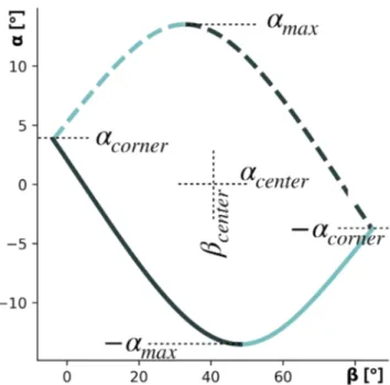
Figure 1. (a) Typical stability field for a wedge with a weak base represented with the surface angle𝛼as a function of the basal angle𝛽. (b–d) Wedge geometry, fault orientation, and orientation of the first principal stress𝜎1for a basal angle of 5◦. (b) The extensionally critical wedge, (c) a stable wedge, and (d) the compressively critical wedge. Parameters are friction coefficient (𝜇 = 0.6), basal friction coefficient (𝜇b=0.3), and fluid overpressure factor (𝜆∗=33%).
wedge shape, the so-called critical taper. The deformation of a pile of sand or snow in front of a bulldozer is a common analog (Dahlen, 1984). We will review the mathematical basis of this theory in section 2.1. Here, we recall some results of this theory in order to set out the reasoning of our present study. For given values of
internal friction𝜇, basal friction 𝜇b, internal fluid pressure factor𝜆, and basal fluid pressure factor 𝜆bthere
is a limited combination of surface angle (𝛼) and basal angle (𝛽) for which the wedge is stable. The stability
conditions, that is, where a wedge deforms only elastically while it slides along its base occur inside the
shaded domain of Figures 1a and 1c. The edges of the curve enclosing the stable (𝛼, 𝛽) region on Figure 1a
correspond to critical taper conditions. In the case where (1 −𝜆b)𝜇b < (1 − 𝜆)𝜇 (weak base), the upper
edge of this curve is the extensionally critical taper characterized by normal faults (Figure 1b), while the lower edge is the compressively critical taper characterized by thrust faults (Figure 1d). In the limit where
(1 −𝜆b)𝜇b= (1 −𝜆)𝜇 (strong base), the stability domain becomes infinitely thin, that is, a line (Figure 2a).
In this particular case, one direction of faulting is parallel to the base which constitutes the ideal condition for underthrusting (Figures 2b–2c). We use the term “neutrally critical taper” to refer to this case.
Contrary to the theoretical prediction that a basal fault needs to be as strong as the wedge material to trigger underplating, natural evidence suggests that plate boundary faults responsible for underthrusting at erosive margins can be very weak. For instance, at the North Chile and South Ecuador erosive margins the middle
Figure 2. (a) The stability field of wedges with a strong base ((1 −𝜆∗
b)𝜇b= (1 −𝜆∗)𝜇) is a line. The taper angle is strongly controlled by the fluid overpressure factor𝜆∗. (b–c) Wedge geometry, fault, and principal stress orientations.
𝜎1is oriented at Coulomb angle to the base, since one direction of faulting is parallel to the base. Thus, it constitutes the ideal conditions for underthrusting. Parameters are friction coefficient (𝜇 = 0.6), basal friction coefficient (𝜇b=0.3), and fluid overpressure factor (𝜆∗=33%).
prisms are typically affected by normal faults which suggest that they are in extensionally critical condition (e.g., Sage et al., 2006; von Huene & Ranero, 2003) and therefore that the basal fault is significantly weaker than the internal wedge strength. The presence of an extensionally critical prism is generally interpreted as the result of a multistep process. First, a wedge with a relatively high taper is built. Then, a reduction of the inner and/or basal effective friction coefficient leads to the taper becoming overcritical. Finally, the wedge deforms to lower its surface angle until reaching the extensionally critical conditions (Cubas et al., 2013; Dahlen, 1984; Wang et al., 2010). Therefore, the presence of normal faults in the middle prism is indicative of a weak plate boundary fault. Gao and Wang (2014) estimated, based on heat flow data inversion that even at erosive subduction margins, that the effective friction coefficient along the plate boundary is less than 0.15. Wang et al. (2010) proposed that theory and observations can be reconciled by considering variations of the plate boundary strength during the subduction earthquake cycle. In their model, they assume that the basal fault is rate strengthening and therefore that underthrusting occurs during earthquakes when the fault is strong, and normal faulting in the prism occurs in the interseismic period when the fault is weak. However, the results of Gao and Wang (2014) suggest that the section of the plate boundary faults that is below the middle prism at erosive margins may remain relatively weak during earthquakes.
In addition to dynamic strengthening or weakening during earthquakes, faults and plastic shear bands also experience permanent weakening caused by, for example, the evolution of rock fabrics (Tesei et al., 2015), fluid pressure increase (e.g., Hubbert & Rubey, 1959; Terzaghi, 1950; Tobin et al., 1994), gouge formation (Burridge & Knopoff, 1967; Dieterich, 1979; Di Toro et al., 2011; Ruina, 1983; Reches & Dewers, 2005; Vrolijk & van der Pluijm, 1999), and stress rotation (Le Pourhiet, 2013; Marone et al., 1992; Marone, 1995; Vermeer & De Borst, 1984). Previous authors showed that weakening controls the effective inner strength of the prism (Lohrmann et al., 2003; Ruh et al., 2012). Here we investigate the control of permanent fault weak-ening on underthrusting, by assuming persistent strain-dependent reduction of friction (in contrast to the cyclic properties proposed by Wang et al., 2010). In agreement with previous studies, we confirm that a strong weakening favors the formation of an extensional wedge. A more surprising result is that this condi-tion also favors underthrusting. The new model that we propose predicts the observed occurrence of coeval permanently weak faults, extensional wedges, and underthrusting.
The goal of this contribution is to determine whether permanent fault weakening promotes or inhibits underthrusting. First, we use the critical taper theory to identify possible structural styles triggered by the transition from an initial intact state to a second state where the internal and/or basal faults have been weak-ened. Second, we perform numerical simulations of deformation of an initially flat layer of plastic material submitted to sandbox-like boundary conditions. Fault weakening was applied to yielded areas using strain softening. The numerical results are consistent with the analytical solution and show a continuum of struc-tural styles ranging from full accretion to full underplating. We discuss the results against analog sandbox experiments and natural examples of underthrusting and gravity collapse.
2. Theoretical Model
2.1. Review of the Critical Taper Theory for a Non-Cohesive Wedge
The critical taper theory was developed through a series of seminal papers in the late 1970s and 1980s (Dahlen, 1984; Dahlen et al., 1983; Davis et al., 1983; Chapple, 1978). The critical taper equations were derived from the equations of stress equilibrium and the Coulomb failure criterion while imposing a shear stress-free condition at the top surface and a critical state of shear stress at the base. In this contribution we propose a simple algorithm to construct the critical taper solution based on results by Lehner (1986). A numerical implementation of this algorithm is given in Appendix B and is available online alongside a set of functions to compute and visualize the solutions of the critical taper equations (Bauville, 2019).
Let us consider a submerged wedge whose surface makes an angle𝛼 with the horizontal (positive
coun-terclockwise). The wedge is bounded at the base by a plane of weakness which makes an angle𝛽 with the
horizontal (positive clockwise) (Figure 1b). The relevant material properties are the densities of the wedge
material (𝜌) and water (𝜌w), and the friction angles (𝜙) or friction coefficient (𝜇 = tan 𝜙) in the wedge and on
the basal plane of weakness (𝜙b, 𝜇b). For a submerged wedge we also define the generalized Hubbert-Rubey
fluid pressure factor in the wedge (𝜆) and at the base (𝜆b).
𝜆 = P𝑓−Pwc
Pwc=𝜌wgD, and (2)
Plitho=𝜌wgD +𝜌gH, (3)
where P𝑓is the fluid pressure at a given depth and Pwcis the pressure associated with the weight of the water
column of height D above the wedge. Plithois the lithostatic pressure, that is, the pressure associated with
the combined weight of the water column and the rock column of density𝜌 and height H. We also define
the hydrostatic pressure Ph𝑦dro=𝜌wg(D + H).
It is convenient to define the fluid overpressure factors𝜆∗and𝜆∗
bthat measure the fluid pressure in excess
of the hydrostatic pressure. It varies from 0 at hydrostatic pressure (P𝑓 =Ph𝑦dro) to 1 at lithostatic pressure
(P𝑓=Plitho).
𝜆∗= P𝑓−Ph𝑦dro
Plitho−Ph𝑦dro, or (4)
𝜆∗= 𝜆 − 𝜆h𝑦dro
1 −𝜆h𝑦dro, (5)
where𝜆h𝑦dro=𝜌w∕𝜌 is the hydrostatic fluid pressure factor.
Next, we define the effective friction coefficients𝜇∗and𝜇∗
bfollowing Wang and Hu (2006)
𝜇∗= (1 −𝜆∗)𝜇, (6)
𝜇∗
b= (1 −𝜆
∗
b)𝜇b, (7)
and another effective friction coefficient𝜇′
bfollowing Dahlen (1984) 𝜇′ b= 𝜇∗ b 𝜇∗𝜇. (8)
Let us also define the effective surface angle (𝛼′) which expresses the ratio of shear stress to surface
orthogonal normal stress (Lehner, 1986),
tan𝛼′= tan𝛼
(1 −𝜆∗). (9)
Finally, we define two intermediate angles (Lehner, 1986) to simplify the final notation.
𝛾 = sin−1 ( sin𝛼′ sin𝜙 ) , (10) 𝜃 = sin−1 ( sin𝜙′ b sin𝜙 ) , (11) where𝜙′ b=tan −1𝜇′ b.
The sum of the surface and basal angles is called the taper angle. When the gravity forces in the wedge balance the frictional forces on the base the taper angle satisfies (Dahlen, 1984; Lehner, 1986)
𝛼 + 𝛽 = 𝜓b−𝜓0, (12)
where𝜓band𝜓0are the angles between the direction of the maximum principal stress𝜎1and the base, and
the surface of the wedge, respectively. Following Lehner (1986) we construct the critical taper envelope by
solving equation (12) for𝛽. The critical taper envelope can be separated in four segments (Figure 3). The two
segments in dashed lines represent solutions where the wedge is extensionally critical while the segments in solid lines represent solutions where the wedge is compressivelly critical. By manipulating equations (9) to (14) of Lehner (1986) we obtain { 𝜓b= 1 2 ( −𝜃 − 𝜙′ b+𝜋 )
, for the upper envelope, 𝜓b= 1 2 ( 𝜃 − 𝜙′ b )
Figure 3. The critical taper envelope is solution of the equation
𝛼 + 𝛽 = 𝜓b−𝜓0. In this equation𝛼is the surface angle,𝛽is the basal angle,
𝜓band𝜓0are the angles between the first principal stress direction and the base or the surface, respectively. One method to construct the critical envelope consists in solving the critical taper equation for𝛽as a function of
𝛼in four segments, here highlighted by combinations of line style and color. Dashed lines denote solutions where the wedge is extensionally critical, while solid lines denote solutions where the wedge is compressively critical. Dashed segments share the same formulation of𝜓b, while solid segments share the same formulation of𝜓0.
The upper and lower envelope is subdivided in two segments represented by light or dark colors in (3), with the relationship
{
𝜓0 = 1 2(−𝛾 − 𝛼
′+𝜋) , for light-colored segments,
𝜓0 = 1 2(𝛾 − 𝛼
′), for dark-colored segments. (14)
Finally, we note that the segments are bounded by values𝛼 = ±𝛼maxand
𝛼 = ±𝛼corner, with
tan𝛼max=𝜇∗, and (15)
tan𝛼corner=𝜇b∗. (16)
A python script implementing this method is given in Appendix B. The implementation has been benchmarked against the graphical solu-tion described in the secsolu-tion “Stable versus unstable wedges” of Dahlen
(1984). Also, one can note that the explicit solution for𝜓b𝜓0 given in
Dahlen (1984) (his equations (9) and (19)) corresponds to the equation for the dark-colored solid segment (Figure 3, equations (13) and (13)). To better understand the variability of the solution note that the
stabil-ity domain has a second order rotational symmetry of center𝛼center, 𝛽center
with 𝛼center=0, (17) 𝛽center= 𝜋 4− 𝜙′ b 2. (18)
The equation of𝛽centerhas the same form as the equation of the Coulomb
angle, that is, the angle at which faults form with respect to the first
principal stress, where𝜃Coulomb=𝜋∕4 − 𝜙∕2. At the left corner
𝛽(𝛼corner) = −𝛼corner, (19) and𝛼 is maximum when
𝛽(𝛼max) =𝛽center−𝛼max+
𝜙 − 𝜃
2 . (20)
2.2. Critical Taper Theory with Fault Weakening
Dahlen (1984) already recognized the strong control that variations in time of the wedge properties
𝜆, 𝜆b, 𝜇, 𝜇b, and𝛽 have on the wedge dynamics. For instance, an initially flat layer of material deforms until it reaches the compressively critical taper. If wedge properties remain constant, it will continue to grow self-similarly. However, if the wedge properties change, it may become either stable, undercritical of over-critical. If the wedge becomes overcritical, then, extensional deformation is triggered, and the wedge taper decreases until it reaches the extensionally critical conditions.
To determine the change in wedge properties necessary to trigger extensional deformation, we consider the evolution of a wedge from an initial intact stage, characterized by the compressively critical surface angle
𝛼0c, to a final weakened stage. We introduce the following two functions:
̄𝛼 = 𝛼 𝛼max , (21) Δ̄𝛼 =𝛼1e−𝛼0c 𝛼max , (22)
where 𝛼1eis the extensionally critical surface angle in the final (weakened) stage. The wedge becomes
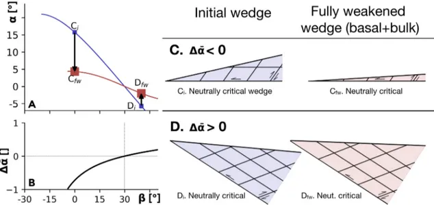
Figure 4. (a) Stability lines of a strong-based (𝜇∗ b=𝜇
∗) wedge (blue line) a fully weakened wedge (red line). The arrow represents the change in surface angle as a consequence of the weakening. (b) Graph ofΔ̄𝛼as a function of𝛽. (c–d) Examples of wedge geometry and fault orientation of the initial and fully weakened wedge in the case whereΔ̄𝛼 < 0(c) andΔ̄𝛼 > 0(d). Parameters are𝜇 = 0.6,𝜆∗=33%, and𝜒 = 80%.
In this section we systematically examine the control of fault weakening, that is, temporal variations of𝜇
and/or𝜇b, on the structural style of accretionary prisms by means of the function Δ̄𝛼. This analysis only
makes use of steady-state solutions and therefore cannot describe the change of kinematics. In a later section of this paper we show numerical solutions that are fully dynamic and adequately describe the kinematics. As we will show later, this simple analysis captures the first order behavior of the dynamic numerical simu-lations. Since we focus on the modalities of underthrusting we restrict the initial conditions to strong-based
cases which is theoretically the ideal condition for underthrusting, that is,𝜇∗
b=𝜇 ∗=𝜇∗
0, where𝜇∗0is a ref-erence effective coefficient of friction (Figure 2). When the wedge is pushed at the rear, it will deform by the formation localized zones of deformation such as faults and plastic shear bands. These localized zones of deformation are generally weaker than the intact material (e.g., Terzaghi, 1950; Tesei et al., 2015; Vermeer & De Borst, 1984). To quantify the impact of fault formation on the wedge dynamics we introduce the
weakening factor𝜒 1 −𝜒 = 𝜇 ∗ 𝑓 𝜇∗ 0 , (23) where𝜇∗
𝑓is the effective friction coefficient of the material inside the fault or shear band.
The critical taper theory predicts the orientation of faults but not their location. As a starting point, it is useful to consider two end-member cases which both evolve from the same initial stage defined above (i.e.,
𝜇∗ b = 𝜇
∗ = 𝜇∗
0initially). One extreme case corresponds to a “fully weakened wedge,” where the wedge
and its base are pervasively faulted, that is,𝜇∗
b = 𝜇 ∗ = 𝜇∗
𝑓. The other extreme case is represented by a
“basally weakened wedge,” where the basal fault is weakened but faulting within the wedge does not lead
to a significant strength decrease. Thus,𝜇∗
b=𝜇 ∗
𝑓, and𝜇∗=𝜇∗0. 2.2.1. Fully Weakened Wedge
Figure 4a shows the stability domains of the initial stage (blue line) and a fully weakened wedge (red line).
In both cases𝜇∗ =𝜇∗
b, therefore, as shown in Figure 2, the stability domains are lines. The function Δ̄𝛼 is
graphed in Figure 4b. When Δ̄𝛼 < 0, the final taper angle is smaller than the initial one (Figure 4c), while
when Δ̄𝛼 > 0, the final taper angle is larger than the initial one (Figure 4c). In the fully weakened wedge
case, the base of the prism is always one of the two possible sliding/faulting directions, which by definition
are oriented at the Coulomb angle ±(𝜋∕4 − 𝜙∕2) from the most compressive stress 𝜎1.𝜎1is correspondingly
inclined with respect to the base. 2.2.2. Basally Weakened Wedge
We now consider a basally weakened wedge, that is,𝜇∗=𝜇∗
0and𝜇∗b=𝜇 ∗
𝑓. A strong-based wedge forms in
Figure 5. Stability fields for a variety of basally weakened wedges illustrating the sensitivity to variables𝜒and𝜆∗.𝜆∗=𝜆∗ b.
free slip, Figure 5). The case where𝜆∗=0%corresponds to a dry wedge or a submarine wedge in which the
fluid pressure is hydrostatic. In the opposite case where𝜆∗=100%, the fluid pressure equals the lithostatic
pressure, and therefore, the internal strength of the wedge goes to zero. Then, the wedge material cannot
support any lateral stress caused by the topography, and therefore,𝛼 = 0◦.
Figure 6a shows the stability domains of the initial wedge (blue line) and a basally weakened wedge (green
area). The function Δ̄𝛼 is graphed in Figure 6b. When Δ̄𝛼 < 0, transitioning from the initial to the weakened
state causes the taper to become overcritical, and therefore, extensional deformation is triggered. Conse-quently, the surface angle is reduced down to the extensionally critical taper conditions of the weakened
wedge (Figure 6c). The black arrow illustrates this process. On the other hand, when Δ̄𝛼 > 0, then the
basally weakened wedge is stable, and therefore, there is no modification of the surface angle (Figure 6d).
Figure 7a shows a graph of̄𝛼 as a function of (1 − 𝜒) for 𝛽 = 0 and 𝜆∗=0. The green area corresponds to the
stability domain of the weakened wedge, while the blue line indicates the surface angle of the intact wedge
(i.e.,𝛼0c, in equation (22)). The dashed and solid green lines indicate the compressional and extensional
critical state solutions, respectively. Thus, Δ̄𝛼 is the signed distance between the solid green and blue lines.
To illustrate the dependence of the surface angle on𝜒 we show two examples. Decreasing the strength of
the basal fault up to𝜒 = 50% should have no incidence because the wedge built at the initial angle remains
stable (red arrow in Figure 7a), that is, the wedge deforms only elastically and slides on its base. This is
specifically true for all values of𝜒 for which Δ̄𝛼 is positive (red arrow in Figure 7a). On the other hand, if
Figure 6. (a) Stability field of a strong-based (𝜇∗ b=𝜇
∗) wedge (blue line) and basally weakened wedge (green area). The green line outlines the extensionally critical taper solutions of the basally weakened wedge. The arrow represents the change in surface angle as a consequence of the weakening. (b) Graph ofΔ̄𝛼as a function of𝛽. (c–d) Examples of wedge geometry and fault orientation of the initial and basally weakened wedge in the case whereΔ̄𝛼 < 0(c) andΔ̄𝛼 > 0(d).
Figure 7. (a) Stability diagram of a basally weakened wedge in the spacē𝛼versus(1 −𝜒)illustrating the control of𝜒on the surface angle of a basally weakened wedge. The wedge has value𝛽 = 0and𝜆∗=0. The dark blue line indicates the surface angle of the intact wedge. The blue and green arrows indicate a hypothetical transition path from an initally intact wedge to a basally weakened wedge. The dashed and solid green lines indicate the compressive and extensionally critical surface angles, respectively. The green area delimits the domain where the wedge is stable. I, II, and III indicate three mechanical modes separated by dashed lines. (b) Contour plot ofΔ̄𝛼as a function of the fluid overpressure factor𝜆∗and the weakening factor𝜒. (c) Contour plot of the mode number functionMassigned as a function of the distance to mechanical mode transitions (black lines).
the basal strength is decreased up to𝜒 = 90% the initial surface angle must become unstable; therefore, the
wedge becomes extensionally unstable. This is specifically true for all values of𝜒 for which Δ̄𝛼 is negative
(red arrow in Figure 7a). A similar analysis was proposed by Willett (1992) and will be discussed later in section 4.1.
Figure 7b shows a contour plot of Δ̄𝛼 as a function of 𝜒 and 𝜆∗, for a constant𝛽 = 0. Based on the value
and variation of function Δ̄𝛼, we can identify three regions or mechanical modes. The boundary between
modes II and III is the zero crossing of function Δ̄𝛼, while the boundary between modes I and II corresponds
to a “ridge” of Δ̄𝛼, that is, a linear local maximum in the represented space. In modes I and II Δ̄𝛼 > 0. In
mode I Δ̄𝛼 increases with increasing 𝜒 and is mostly independent of 𝜆∗, while in mode II, Δ̄𝛼 decreases with
increasing𝜒 and and 𝜆∗. In mode III Δ̄𝛼 < 0 and it decreases with increasing 𝜒.
In modes I and II Δ̄𝛼 > 0, therefore, the initial wedge is predicted to be stable in the weakened conditions
(as in Figure 6d). On the contrary, in mode III the initial wedge is overcritical and must deform to reach the extensional critical taper of the weakened wedge (Figure 6c). The critical taper theory alone does not predict a structural style difference between modes I and II. To overcome this shortcoming and to obtain more information about the structural style of underthrusting-dominated wedges, in the following section
we present a set of numerical simulations that cover the parameter space presented in Figure 7a. Δ̄𝛼 > 0
does not increase monotonically across the parameter space. Therefore, to ease the representation of results in the following sections, we introduce the monotonic function “mode number” M (Figure 7c). M = 1 at
𝜒 = 0; M = 2 at the transition between the modes I and II; M = 3 at the transition II∕III, and M = 4 at 𝜒 = 100% and 𝜆∗= 100%. M is interpolated linearly between mode transitions to cover all the parameter space.
3. Numerical Simulations
In this section, we first give an overview of the numerical methods and initial configuration before presenting the simulation results. The numerical results are presented in the context of the theoretical predictions.
3.1. Methods
3.1.1. Numerical Method
The numerical algorithm solves the Stokes equations that describe the flow of rocks over a geological time scale. The software is based on finite-difference marker-in-cell method (Harlow & Welch, 1965;
Figure 8. Schematic diagram of the initial configuration and boundary conditions. Boundary conditions are (top) free surface (sticky air); (right) no slip; (left)
free slip and constant horizontal velocity Vx = Vpush; (bottom) vertical velocty Vy = 0, horizontal velocity Vx = Vpush.
Gerya & Yuen, 2003). All invariants are computed on a staggered grid. The system of equations is solved for
vx, v𝑦and P using the implicit direct solver PARDISO v6.0.0 (De Coninck et al., 2016; Kourounis et al., 2018;
Verbosio et al., 2017). The viscous term is effectively switched off by using a very high viscosity. We chose the time step size such that it takes at least one to two time steps to build enough elastic stress to reach the yield stress. The plastic rheology follows a non-associative flow rule. We describe the governing and constitutive equations in details in Appendix A.
Here, we give a brief description of the strain weakening algorithm. The yield stress is defined by the Mohr-Coulomb relation,
𝜏𝑦=Ccos(𝜙) + (1 − 𝜆)(P − Pwc)sin(𝜙), (24)
where C is cohesion,𝜙 is the friction angle, 𝜆 is a fluid pressure factor, P is the pressure, and Pwcis the
weight of the overlying column of water. The standard yield function for a Mohr-Coulomb failure criterion
is defined as F =𝜏II −𝜏𝑦≤ 0, where 𝜏IIis the second invariant of the stress tensor. Here instead the yield
function is defined according to the weakening factor𝜒, such that
F =𝜏II− (1 −𝜒w(𝜖p))𝜏𝑦, (25)
𝜖pis the second invariant of the cumulated plastic strain, and w(𝜖p)is a piecewise linear weighting function
which takes values 0 for 0< 𝜖p< 0.5 (no weakening) and 1 for 𝜖p> 1 (maximal weakening). w(𝜖p)increases
linearly from 0 to 1 for 0.5 < 𝜖p< 1. 3.1.2. Model Configuration
The model configuration mimics a 2D sandbox experiment (Figure 8). We set a homogeneous layer of
sed-iment of constant thickness of H. For all simulations the size of a single cell is dx =d𝑦=H∕64. The basal
angle is𝛽 = 0◦all along the present study. The layer is dragged from below and pushed at the left boundary
against a fixed backstop (right boundary). At the left boundary the horizontal velocity vx = vpush, and the
vertical velocity v𝑦remains such that the shear stress𝜎x𝑦=0(free slip). At the bottom boundary v𝑦=0and
vx =vpush. At the top boundary of the numerical domain,𝜎x𝑦= 0and v𝑦balances the inbound flow from
the left boundary. At the right boundary vx = v𝑦 = 0(no slip). Displacement along the right boundary is
accomodated either by backthrust faults or by plastic shear zones at the boundary, developing early in the simulation. This equivalence has been verified a posteriori by the agreement between the numerical model and the analytical solution wherein a stress condition is specified at the boundary (Buiter et al., 2006, 2016). On top of the sediment layer we set a layer of sticky water, that is, a layer of very low viscosity with a
den-sity of 1,000 kg/m3, such that the surface of the sediment layer is effectively shear stress-free (i.e., vertically
loaded free surface, Crameri et al., 2012). The sediment has a density of 2,500 kg/m3, and the shear modulus
is such that in the initial conditions, the strain necessary to reach the yield stress at a depth H (i.e., which
corresponds to the base of the model at the beginning of the simulation) is𝜏𝑦∕(2G) = 1%. The friction angle
is𝜙 = 30◦. In the absence of cohesion, stress vanishes at the surface which can cause a very large velocity. To avoid this situation, we use a small value of cohesion. For each simulation, this value is chosen such that
the thickness of the cohesive boundary layer is Hc=H∕32, that is, two cells, with
Hc= C
(1 −𝜆)𝜌g𝜇, (26) where g is the acceleration of gravity.
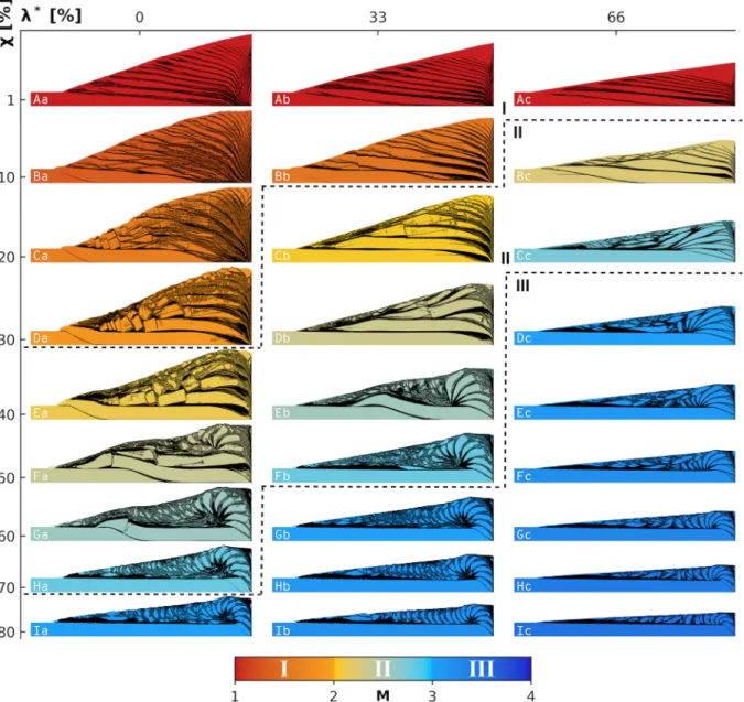
Figure 9. Wedge geometry (color) and fault geometry (black) for a set of 27 simulations with systematic combinations of𝜒and𝜆∗. The wedge material is color-coded according to the theoretical mode numberM. Colors are darkened according to plastic strain. The theoretical boundary between modes is indicated by dashed lines.
3.2. Results
3.2.1. Systematic Analysis
Figure 9 presents a set of 27 numerical simulations for𝛽 = 0, 𝜒 = 1, 10, 20, 30, 40, 50, 60, 70, 80% and 𝜆∗=
0, 33, 66%. Each simulation is shown at a different time such that the front of the wedge (i.e., its leftmost extent) is at a similar position and the surface is close to a stable taper for each simulation. The wedge material is colored according to the theoretically determined mode number M. Zones of high plastic strain, that is, faults, are shaded in black. The axes and the colormap are the same as in Figure 7b. Below we use the term tectonic slice or nappe to describe a large sliver of sediment bounded by two parallel faults. First, we can define three archetypal tectonic styles.
Style 1 (M ≈ 1) is characterized by oblique closed spaced long thrusts that define a stack of thin slices (Figures 9Aa–9Ac). Style 2 (M ≈ 2) is characterized by nappe stacking with nappes as thick as the incoming sediment. There is a highly deformed region near the surface similar to a slope apron (Figures 9Ea, 9Db, and 9Bc). Style 3 (M ≈ 3) is characterized by an intensely deformed prism overlaying undeformed incoming sediments. The prism is composed of a rear region with short tectonic slices arranged in a spiral fashion, and a frontal region where those slices have been reworked by extensional tectonics (Figures 9Ia, 9Gb, and 9Dc).
(a)
(b)
(c)
Figure 10. Wedge geometry (colors) and fault geometry (black) of the three simulations archetypal of the tectonic styles. Colors are passive markers of the
deformation and are darkened according to plastic strain.𝜆∗=33%for all simulations. (a) Style 1,𝜒 = 1%; (b) Style 2,𝜒 = 20%; and (c) Style 3,𝜒 = 60%. Simulations with intermediate values of M have tectonic styles that share characteristics with the bracketing
archetypal styles. Simulations with 1 < M < 2 are characterized by less well-defined thrust planes with
anastomosing faults (Figures 9Ba and 9Bb), and thicker tectonic slices (Figures 9Ba and 9Ca). Simulations
with 2 < M < 3 feature a combination of the long tectonic slices characteristic of Style 2 and the short
spiraling slices characteristic of Style 3 (e.g., Figures 9Fa, 9Ga, and 9Eb). The intensity of tectonics also increase gradually from M = 2 to M = 3 (e.g., Figures 9Ea–9Ha). From M = 3 to M = 4 the distinction between the front and rear sections of the wedge tends to disappear as the extensional reworking the of the tectonic slices decreases in efficiency. An archetypal Style 4 could have been defined, corresponding to the case𝜒 = 100% and a top surface slope parallel to the base.
Simulations with the same mode number M but different combinations of𝜒 and 𝜆∗share many
characteris-tics but also show differences. In simulations where𝜆∗=0%and 1< M < 2, tectonic nappes are internally
faulted (Figures 9Ba–9Da). The frontal part of the prism can also be reworked by normal sense faulting in a
domino tectonics fashion (Figures 9Ba and 9Ca). Simulations where𝜆∗=33%show significantly less
inter-nal faulting of the slices (Figure 9Cb), and simulations where𝜆∗ =66%do not show any. The simulation
where𝜒 = 10% and 𝜆∗=66%(Figure 9Bc) is classified as Style 2 but does not show the characteristic thrusts
parallel to the base since the simulation is shown at a relatively early and immature stage. For comparison,
in the simulation where𝜒 = 20% and 𝜆∗=33%(Figure 9Cb), the earliest tectonic slices (highest in the pile)
are also not parallel to the base. We consider simulations at𝜆∗=33%and𝜒 = 1%, 𝜒 = 20% and 𝜒 = 60%
to be the most archetypal of Styles 1, 2, and 3, respectively. Therefore, in the following sections, we focus on these three simulations.
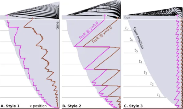
Figure 11. Horizontal position of the forelandmost (i.e., leftmost) fault as a function of time. The wedge and fault
geometry of the three simulations attre𝑓are reproduced above the graph.𝜆∗=33%for all simulations. (a) Style 1,
𝜒 = 1%; (b) Style 2,𝜒 = 20%; and (c) Style 3,𝜒 = 60%. 3.2.2. Time Evolution of End-Members: Geometry
In the previous section, we described the geometry of tectonic structures qualitatively at a given time. In this section, we describe the evolution of structures in time, and we attempt to characterize them furthermore by monitoring the position of faults and the surface slopes through time.
In Style 1 a new thrust is recurrently formed, connecting the front of the prism to the bottom right corner of the box (Figure 10a). These frequent thrusts define thin tectonic slices. Since the frontal thrusting frequently occurs the surface angle appears relatively constant, and the surface is relatively planar. At a later stage
(Figure 10, A.tre𝑓) the rear segment of the frontal thrust runs along the base of the sediment.
In its early stage, Style 2 is similar to Style 1 with new faults cutting the sediment obliquely to connect the
front of the wedge to the corner of the box (Figure 10, B.t1). However, from time t2the full sediment thickness
is incorporated into nappes. For instance, the purple material is incorporated down to its base in the lowest
tectonic slice (Figure 10, B.t2). The sequence from time t5to tre𝑓exemplifies the creation of a tectonic nappe
(Figure 10, B.t6–B.tre𝑓). A frontal thrust appeared slightly before t6. At t6the incoming material is indenting
into the material of the nappe. As a consequence, the nappe material is carried up over the ramp formed by
the former frontal thrust and the incoming material is underthrusted below. Figure 10 (B.t7) shows a typical
flat-ramp-flat geometry. At tre𝑓the former frontal thrust has reached the backstop. The nappe is completely
uplifted, and a new frontal thrust will form soon after to incorporate more material in the wedge. Superficial
collapse starts being active from t2, with recurrent normal faulting over shallow depths. The slope apron
keeps on developing until tre𝑓, although its thickness remains fairly constant.
The dynamics of Style 3 can be described in three stages. In the first stage (Figure 10, C.t1–C.t2), incoming
sediments are faulted to form tectonic slices that are exhumed against the backstop. The exhumed slices are cut again by normal faults. An upper wedge made of normal faulted tectonic slices forms. In the second
stage (Figure 10, C.t3–C.t5), normal faults do not cut through the entire wedge but affect only a restricted
region near the surface. Tectonic slices are exhumed and push toward the front of the upper wedge without being completely normally faulted. The stacked nappes are arranged in a spiral fashion. In the first two stages, the paleo-surface of the incoming sediments constitutes the base of the wedge. In the third stage
(Figure 10, C.t6–C.tre𝑓) a new décollement forms within the wedge to become the new base of the wedge.
The new décollement dips toward the foreland,𝛽 ≈ −4◦at t7and𝛽 ≈ −2.5◦at tre𝑓. The most striking feature
Figure 12. Evolution of the surface angle as a function of time. The colors code for the peak intensity of the surface angle histogram computed for each
simulation time step. The theoretical stability range of the basally weakened wedge, intact wedge, and fully weakened wedge are also represented.𝜆∗=33%for all simulations. (a) Style 1,𝜒 = 1%; (b) Style 2,𝜒 = 20%; and (c) Style 3,𝜒 = 60%.
pile that is underthrusted below it. Movies of the evolution of the geometry and surface angles of these three simulations are available in supporting information Movies S1–S3.
3.2.3. Time Evolution of End-Members: Faults' Position
In the previous section, we described the geometry of the wedge qualitatively. In the following two sections we characterize the structural style by monitoring scalar values through time. The values we use are the outermost fault position at a given depth (Figure 9), and the surface angle (Figure 10).
Figure 11 shows a graph of the horizontal position of the forelandmost (i.e., leftmost) fault at a given depth (x-axis) as a function of time (y-axis). The wedge geometry and fault geometry of each simulation are
represented above the graph at tre𝑓for reference. We graphed the fault position at depth𝑦 = 0.8 (magenta
line) and𝑦 = 0.0 (brown line). We term these positions, shallow fault position, and basal fault position,
respectively. The grayed area in the graph corresponds to the area to the right of the wedge's front. The times
t1to tre𝑓indicated by gray lines correspond to the time steps shown in Figure 10.
In Style 1, the shallow fault position always remains close to the front position (Figure 11a). Sudden varia-tions in the fault position indicate the formation of a new fault in a more frontal position. The basal fault position marks the same cycle of new fault formation and additional small oscillations. The basal fault
posi-tion remains close to the backstop until t2, after which the basal fault position gradually becomes closer
to the front. Through the oscillation cycle, the basal fault's position never returns toward the backstop. It means that through time an increasing portion of the base is permanently faulted.
In Style 2, there are cycles where a new fault is formed and then pushed toward the back by incoming sedi-ment (Figure 11b). Once the basal fault position reaches the backstop, a new fault forms. When the new fault forms the shallow fault position is at the front, and the basal fault position is a bit behind. This configura-tion expresses that when a new fault forms, the fault develops at the base forming a basal décollement from
which a frontal thrust steps up (see also B.t6). At the beginning of the cycle almost all the base is faulted,
while at the end, none of it is.
In Style 3, both the shallow and basal front position remain close to the backstop. Similarly to Style 2, a new fault is created when the basal position reaches the backstop. In Styles 1 and 2 the most frontal position of both the shallow and basal fault position follows the advance of the front. However, in Style 3 the position of the fault is independent of the position of the front. The position of the faults near the backstop reflect the regular formation of short tectonic slices.
3.2.4. Time Evolution of End-Members: Surface Angle
Figure 12 presents the time evolution of surface slope for the three end-member simulations. For each time step, the figure presents a histogram of surface slopes. The intensity of the peaks of the histogram is color-coded. To construct this graph, at a given time step we measure the slope at all cell centers defining
the surface by performing a least squares regression over topography points over a width 0.5H before and
after the cell considered. Then, we construct the histogram of the surface slopes at a given time step. The final graph is composed of many histograms, one for each time step, shown next to each other. We also
rep-resent the graph of the shallow fault position (fault@𝑦 = 0.8), given here without scale, to inform the reader
on the relation between the surface slope and faulting activity. Over each graph we represent the theoret-ically determined stability domains of the intact basally weakened and fully weakened wedge. The intact wedge stability domain is a line identical for all simulations. The weakened wedges stability domains are
controlled by𝜒 and 𝜆∗, and therefore, they are different for each simulation.
This graph offers a representation of the distribution of local surface slopes in the wedge. Because of the distribution of faults, the mechanical properties (e.g., basal friction) are not homogeneous, and therefore, the slope distribution is often multimodal. The link between multimodal slope distribution and basal faulting
can also be observed in Figure 10 (t4and t6).
Style 1 shows first a period of slope increase accompanied by oscillations associated with fault activity
(Figure 12a). Around time t2the slope becomes asymptotic toward the intact or the fully weakened
stabil-ity line. Note that since𝜒 = 1% both lines nearly overlap. After time t3the distribution is bimodal. Part
of the wedge oscillates around the intact stability line. Another part of the wedge shows oscillations which peak at the compressively critical state of the basally weakened wedge (i.e., the lower envelope of the green domain). The peak of the oscillations coincides with the formation of a new frontal thrust. Looking back
at the wedge geometry (e.g., Figure 10, A.t7) we observe that the bimodal distribution arises from the
con-vex upward surface. Indeed, the surface slope of the forelandmost half of the wedge is a few degrees steeper than the rearmost half. This dichotomy is likely a consequence of the rearmost part of the base always being faulted, that is, weakened, as shown in Figure 11a.
Style 2 also shows first a period of slope increase that stops before time t1when the slope reaches the
exten-sionally critical condition (Figure 12b). At time t1the first event of décollement propagation and frontal
thrust formation occurs (see also Figure 11b). This faulting event triggers a rapid decrease of the surface slope. Up to now, the slope distribution was unimodal. However, after the slope has decreased to about the
level of the intact wedge stability line between time t1and t2, the distribution becomes bimodal. Part of the
wedge's slope continues to decrease until it comes close to the compressively critical state, while another part of the wedge increases until it reaches the extensionally critical state. Each major faulting event
trig-gers similar patterns. This multimodal distribution is also clear in, for example, Figure 10 (B.t3–B.t7). As in
Style 1, the frontal part of the prism is steeper than the rear part. It appears clear that the landslide type sur-face tectonics coincides with the steeper portions of the wedge and must be triggered when the local sursur-face
slope reaches the extensional condition. Although the slope distribution is always multimodal, after time t5
it becomes clear that some peaks in the distribution become asymptotic. At the end of the simulation, the
asymptotic peaks are 1–2◦above the intact wedge stability line. Nevertheless, we expect the distribution to
become bimodal again after a new frontal thrusting event.
In Style 3, the slope distribution first increases and reaches a peak above the intact wedge stability line. At this point the distribution becomes bimodal with part of the distribution oscillating around the extensionally
Figure 13. Simulation representative of mechanical mode III (𝜆 = 33%,𝜒 = 60%) with an initial taper. (a) Evolution of the surface angle as a function of time. The colors code for the peak intensity of the surface angle histogram computed for each simulation time step. The theoretical stability range of the basally weakened wedge, intact wedge, and fully weakened wedge are also represented. (b) Wedge geometry (colors) and fault geometry (black). Colors are passive markers of the deformation and are darkened according to plastic strain.
critical state of the basally weakened wedge while another, stronger peak becomes asymptotic toward the fully weakened wedge stability line. Hence, at an advanced stage, because the wedge is intensely faulted,
it effectively behaves as if it was completely weakened (see also Figure 10, C.tre𝑓). Faulting events control
oscillations of the slope distribution peak close to the extensional state of the weakened wedge, while the asymptotic portion of the distribution is mostly unaffected by faulting events. We interpret that the first peak can reach a value higher than the intact stability line because the base of this small wedge is effectively the
lowest thrust which dips at 15◦at time t1(Figure 10, C.t1).
3.2.5. Influence of Initial Conditions
In Figure 13 we show the evolution of angles and geometry for a simulation with𝜆 = 33%, 𝜒 = 60%, where
a wedge with a surface angle of 10◦is initially present near the backstop. This initial wedge has a surface
angle lower than the stability angle of the intact wedge but higher than the stability angle of a fully weakened
wedge (Figure 13a and B.t1). First, a frontal thrust is created soon after time t1. The material uplifted along
the ramp is extensionally critical (Figure 13a) and therefore deforms by normal thrusting (Figure13, B.t2).
Subsequently, normal thrusts affect domains closer and closer to the backstop and a secondary décollement
parallel to the surface forms from time t3to t5. These normal faults reduced the surface angle from 10◦
initially to 7◦where the peak of the surface angle distribution reaches a steady state (Figure 13a). This angle
is comparable to the steady-state angle for Style 3 shown in Figure 12c. The ramp reaches the backstop at
time t4, and from t4to t6the incoming material is deformed in small slices updated along the backstop in a
spiral fashion similar to what we observed in Style 3 (Figure 10c). Between time t6and t7a new basal thrust is
created, but the ramp is created below the wedge and doesn't reach the front. The material behind the ramp is then uplifted in a new event of underthrusting. The formation of a long nappe with a fault that ramps up in the middle of the wedge was not observed in our simulation characteristic of Style 3 (Figure 9Gb) but is observed in simulations of mechanical mode II (e.g., Figures 9Fa, 9Ga, and 9Eb). Normal faulting is the dominant mode of deformation in the material that composed the initial taper, while material accreted after the first ramp reached the backstop is deformed in short slices that are exhumed in a spiral pattern typical of Style 3. Long slices also formed in this simulation suggesting that the boundary between mechanical modes
II and III occurs for smaller𝜒 or 𝜆 compared to the case without initial taper. It seems reasonable to assume
that for a higher value of𝜒, only small slices would form, similar to what is observed in Figure 9.
A movie of the evolution of the geometry and surface angles of this simulation is available in Movie S4.
4. Discussion
4.1. Control of Fault Weakening on Accretionary Prism Dynamics
We demonstrated above the first order control of fault weakening on the structural style for strong-based accretionary prisms. Previous researchers have also investigated the control on fault weakening of the dynamics of accretionary prisms. Such studies showed that fault weakening favors the localization of shear zones, increases the displacement on individual faults, and increases the thickness of thrust sheets (Ellis et al., 2004; Selzer et al., 2007). Willett (1992) investigated the kinematics of a wedge subject to changes in
basal friction using numerical methods. In one of his simulations which is initiated with𝜙b = 𝜙 = 30◦,
Willett (1992) describes the formation of a thrust that connects the front of the model to the corner of the box, such that the material is partially underplated. A moderate decrease of basal friction, such that the wedge moves into the stable field, triggers accretion rather than underplating of the material, reducing the surface angle. Then, a further decrease of basal friction triggers the gravitational collapse of the wedge. These three stages of Willett's (1992) simulation correspond to the three mechanical modes described in our present study. However, in Willett (1992), the reduction in basal friction is applied along the lower(basal) boundary, whereas it decreases dynamically along all faults in our models. In contrast to that specific case from Willett (1992), we observe the formation of an antiformal nappe stack (Style 2) and oscillations of the surface slope with cycles of frontal thrust formation and underplating. A further decrease of basal friction (i.e., mode III) in Willett's (1992) case triggers the gravitational collapse of the wedge, which contrasts sharply with our models in which a complete underthrusting of the incoming sediment with exhumation against the back-stop occurs (Style 3). The differences between the two studies outline a fundamental difference between mechanical mode based on the critical taper theory and the structural style which depends on boundary conditions and faulting dynamics.
In another simulation Willett (1992) starts from a situation where 𝜙b < 𝜙. The author then applies
Figure 14. Contour plot ofΔ̄𝛼as a function of the fluid overpressure factor𝜆∗and the weakening factor𝜒at𝛽 = 0. Color shaded squares indicate the range of parameters𝜒and𝜆∗expected in dry (red) and overpressured (orange) analog sandbox experiments, and in nature (green). All three mechanical modes I, II, and III can be expected in nature. In dry sandbox experiments only mode I and II can be reached, while mode III may be reached in overpressured analog sandbox experiments.
compressively critical. In another study, Ruh et al. (2012) used numerical simulations in which fault weak-ening was allowed in the wedge but not along its base. As a result, the authors observed an increase in surface angles in response to an effective decrease of the coefficient of friction in the wedge, in agreement
with the observations by Willett (1992). The case of an increase in basal friction (𝜙b) or a decrease in the
wedge strength (𝜙), without decreasing the basal strength, is not the purpose of our present study (which
we chose to focus on the case𝜙b=𝜙).
4.2. Comparison With Sandbox Experiments
Analog sandbox experiments have been used extensively to study the dynamics of accretionary prisms (for recent reviews, see Buiter, 2012; Graveleau et al., 2012; Schreurs et al., 2016). Sandbox experiments are often
performed in subaerial (dry) conditions, that is,𝜆∗=0, and the sands used in experiments are estimated to
have a weakening factor𝜒 ≈ 2 − 26% if the difference between peak and reactivation friction coefficient is
considered, or𝜒 ≈ 10−44% if instead the difference between peak and dynamic friction coefficient is
consid-ered (Klinkmüller et al., 2016) (Figure 14). Therefore, our results predict that sandbox experiments should
feature Styles 1 to 2 for𝛽 = 0◦. This prediction is in agreement with the observation that sandbox
experi-ments with a strong base (𝜙b≈𝜙) are characterized by long thrust sheets and antiformal nappe stacks (e.g.,
Adam et al., 2005; Del Castello & Cooke, 2007; Gutscher et al., 1996, 1998; Huiqi et al., 1992; Malavieille, 2010). A similar structural style arises in numerical simulations using the discrete element method (Burbidge & Braun, 2002). The model also predicts that Style 3 may be achieved in a sandbox for negative
values of𝛽. Sandbox models typically do not show the kind of domino deformation displayed in our models
when𝜆∗=0%(Figure 9), but more closely resembles the style of simulations that we obtain for𝜆∗=33%.
These differences may have a few main causes. First, in analog experiments the basal friction is never as high as the internal friction. Second, sand can compact and dilate whereas in our model is incompressible
with nonassociated plasticity (i.e., the dilation angle is zero). Finally, the weakening algorithm we employ is a simplification of the strain weakening that applies to sand.
Some researchers have investigated the control of fluid pressure in analog sandbox experiments using
com-pressed air flow (Cobbold & Castro, 1999; Cobbold et al., 2001; Mourgues & Cobbold, 2006). Values of𝜆∗as
high as 0.8–0.9 can be reached (Mourgues & Cobbold, 2006; Pons & Mourgues, 2012). Therefore, it seems theoretically possible to reproduce the results of this study with an analog apparatus (Figure 14). However, to the knowledge of the authors, experiment with an initially strong base, and high fluid pressure that could generate Style 3 have not been performed yet.
4.3.𝝀∗and𝝌 in Nature
The pore fluid pressure factor𝜆 and pore fluid overpressure factor 𝜆∗have been estimated in natural
accre-tionary prism using a variety of methods. A review of those methods and results is given by Saffer and Tobin (2011). Generally the fluid overpressure in accretionary prisms is relatively high. Borehole-based studies
indicate that within 1–4 km of the trench,𝜆∗ = 0.20 − 0.91 within underthrusting sediment. Recently,
Flemings and Saffer (2018) have estimated the fluid pressure in the Nankai accretionary prism from
poros-ity measurements with a critical state soil model. They determined that𝜆∗=0.7−0.9 for a range of assumed
friction angles between 5◦and 30◦(Figure 14).
The weakening factor𝜒 can be associated with several mechanisms in nature. First, highly reflective
décolle-ments in seismic reflection data are often interpreted as resulting from elevated pore fluid pressure localized on the décollement (Bangs et al., 2009; Park et al., 2002, 2010; Ranero et al., 2008). For instance, Tobin et al.
(1994) estimated that𝜆∗=0.86−0.98 along the frontal thrust of the central Oregon margin, based on seismic
reflection waveform, amplitude modeling, and laboratory measurements on core samples. In rocks rich in both carbonate and clay minerals, the departure of calcite during the early stages of faulting play an impor-tant role in the early weakening of faults (Lacroix et al., 2015). This weakening mechanism is associated with the development of a slaty fabric. Tesei et al. (2015) measured the friction coefficient of fault material
from clay-rich sediment. They measured friction coefficients𝜇 = 0.17 − 0.26 in fault rocks showing a slaty
cleavage, whereas powders made of the same material and representative of the material without fabric had
𝜇 = 0.49 − 0.55. The strength reduction due to fabric formation correspond to 𝜒 = 60 − 65% (Figure 14).
Other mechanisms include the formation of clay gouge and the associated dynamic metamorphism that triggers the transformation of illite into smectite (Reches & Dewers, 2005; Vrolijk & van der Pluijm, 1999), the process of dynamic weakening during earthquakes (Burridge & Knopoff, 1967; Dieterich, 1979; Di Toro et al., 2011; Ruina, 1983), or the decrease of effective stress due to the shearing or thinning of a shear zone (Le Pourhiet, 2013; Scott et al., 1994).
These estimates of𝜒 and 𝜆∗from natural examples indicate that mechanical mode III is likely to be reached
in nature. However, whether mechanical mode III would be expressed as structural Style 3 is not clear and would depend on boundary conditions. The spiral pattern characteristic of Style 3 is not observed in nature as far as the author knows. In nature mechanical mode III deformation of the backstop may allow all the material to be subducted instead of forming the spiral pattern characteristic of Style 3. Further study is necessary to test this hypothesis.
4.4. Applicability to Natural Structures 4.4.1. Nappe Stacking
Antiformal nappe stacks are essential structures in fold-and-thrust belts and accretionary prisms. Examples are the Helvetic nappes in Switzerland (Escher et al., 1993) or the Alberta foothills in Canada (Fermor & Moffat, 1992). The base of tectonic nappes is often composed of mechanically weaker horizons. In this case, the applicability of our model is limited, and models incorporating several weak layers are more appropriate to reproduce these structural styles (Massoli et al., 2006; Ruh et al., 2012). On the other hand, the mecha-nism of dynamical weakening described in our study can explain nappe stacks where no particularly weak horizons are present, such as in the accretionary prism of the Aleutian Trench (Gutscher et al., 1998). Our results suggest that in these conditions the formation of an antiformal nappe stack is restricted to mechanical conditions that are close to the transition between modes I and II.
4.4.2. Slope Aprons and Olistostrome
In our numerical models we observe shallow gravity instabilities /similar to slope aprons/ for simulations in mechanical modes II and III. This result is consistent with the prediction of Mourgues et al. (2014). In their
which varies very similarly tō𝛼. When those numbers are close to 1, shallow gravity sliding occurs. When
FSor ̄𝛼 decreases, Mourgues et al. (2014) suggest that deep normal faults reaching the décollement are expected. This theoretical prediction is consistent with the transition that we observe from shallow gravity sliding in Style 2 to deep normal faulting in Style 3.
Style 3 could explain the formation of olistostromes and submarine landslides. A complementary question in this regard is whether extensional faults are mostly planar in the third direction, or whether they are curved and thus define lentils as is commonly observed for gravitational instabilities. In our model, we neglected inertia and employed a certain cohesion to limit the minimum strength of rocks near the surface. Without this limitation, gravitational instabilities would rapidly run down the surface slope. It would thus form submarine landslides.
4.4.3. Erosive Margins/Subduction Channel
Subduction channels have been imaged, for example, in Chile, Costa Rica, Nicaragua, or Ecuador (Ranero et al., 2008; Sage et al., 2006; von Huene & Ranero, 2003). Several authors have proposed a sandbox configu-ration that models the development of basal erosion and the formation of a subduction channel. It consists of a preexisting initial wedge and an incoming horizontal sediment layer. An outflow is allowed through a “subduction gate” located below the backstop (Albert et al., 2018; Gutscher et al., 1996, 1998; Kukowski & Oncken, 2006). These studies showed that in high-basal-friction conditions, a subduction channel forms spontaneously (Gutscher et al., 1998; Kukowski & Oncken, 2006). The shape can vary as a function of the outflow (Albert et al., 2018). These experiments suggest that given appropriate initial and boundary con-ditions, the mechanical modes I and II result in the formation of a subduction channel rather than the antiformal stack characteristic of Style 2. Our results suggest that a subduction channel also tends to form spontaneously in mechanical mode III, although this hypothesis remains to be validated, for example, by performing simulations with the initial and boundary conditions cited above.
4.5. A General Mechanism for Style 3
The mechanical behavior of mechanical mode III is mostly controlled by the fact that the surface angle is such that the upper wedge is critically neutral, but the incoming material is always in the undercritical regime. The wedge needs to reach the critical taper to overcome basal shear stress and initiate displacement along the base. Since the regime is undercritical in the incoming sediment, this condition is never met, and the material is instead underthrusted below the weak wedge. The material only deforms against the backstop because there, the stress field is forced to reach the yield state. Once the material reaches the backstop, it can only go up and is therefore exhumed. In our model, the taper remains undercritical because of pervasive deformation and fault weakening. Surface processes, that is, erosion and sedimentation, can also control the slope so that the taper remains undercritical (Willett, 1999). Therefore, surface processes can also favor deformation at the back/rear rather than at the front (Simpson, 2010) and trigger exhumation (Burbank, 2002; Dahlen & Suppe, 1988; Malavieille & Konstantinovskaya, 2010; Mary et al., 2013).
4.6. Limits of the Method
Many processes in nature can cause weakening of faults. We did not model the physics of these processes, but instead we used a standard parameterization of strain softening that links plastic strain to a weakening factor (equation (25)). This numerical scheme is often used but has the important caveat of being mesh-sensitive. In this study, all simulations have been performed at the same resolution such that simulations are consistent with each other. Furthermore, we performed a test to assess the sensitivity of the structural style on the numerical resolution (Figure 15). We ran the characteristic simulations of Styles 2 and 3 at resolution of
H∕16, H∕32, H∕64 (i.e., default), and H∕128. The test reveals that resolution has some impact on the location
and angle of faults as shown in Kaus (2010). At the lowest resolution (H∕16) it seems that the structural style changes through time. However, this artefact disappears at higher resolution. For resolution greater than H∕32 the resolution does not influence the characteristics of the structural style such as the surface angle, shallow surface instabilities, gravitational collapse, underthrusting, exhumation, or antiformal nappe stacking. The simulation with an initial taper outlines the fact initial conditions affect the structural style, even though the overall kinematics remains similar to a case without initial taper. Furthermore, testing the control of backstop deformation on the structual style is out of the scope of this study, but it is without a doubt an important factor and may allow the incoming material to be completely underthrusted instead of being accreted at the base of the prism in a spiral pattern as it is the case here.