Accepted Manuscript
Research papersRegional Frequency Analysis Using Growing Neural Gas Network Amin Abdi, Yousef Hassanzadeh, Taha B.M.J. Ouarda
PII: S0022-1694(17)30267-6
DOI: http://dx.doi.org/10.1016/j.jhydrol.2017.04.047
Reference: HYDROL 21978
To appear in: Journal of Hydrology Received Date: 9 October 2016 Revised Date: 21 February 2017 Accepted Date: 20 April 2017
Please cite this article as: Abdi, A., Hassanzadeh, Y., Ouarda, T.B.M., Regional Frequency Analysis Using Growing Neural Gas Network, Journal of Hydrology (2017), doi: http://dx.doi.org/10.1016/j.jhydrol.2017.04.047
This is a PDF file of an unedited manuscript that has been accepted for publication. As a service to our customers we are providing this early version of the manuscript. The manuscript will undergo copyediting, typesetting, and review of the resulting proof before it is published in its final form. Please note that during the production process errors may be discovered which could affect the content, and all legal disclaimers that apply to the journal pertain.
1
Regional Frequency Analysis Using Growing Neural Gas Network
Amin Abdi1*, Yousef Hassanzadeh1, Taha B.M.J. Ouarda2, 3
1
Department of Civil Engineering, University of Tabriz, Tabriz, Iran
2
Institute Center for Water and Environment, Masdar Institute of Science and Technology, Abu Dhabi, UAE
3
National Institute for Scientific Research, INRS-ETE, Quebec (QC), Canada
February 20th 2017
*
Corresponding author. Tel.: +98 413 339 2395.
2
Abstract
The delineation of hydrologically homogeneous regions is an important issue in regional hydrological frequency analysis. In the present study, an application of the Growing Neural Gas (GNG) network for hydrological data clustering is presented. The GNG is an incremental and unsupervised neural network, which is able to adapt its structure during the training procedure without using a prior knowledge of the size and shape of the network. In the GNG algorithm, the Minimum Description Length (MDL) measure as the cluster validity index is utilized for determining the optimal number of clusters (sub-regions). The capability of the proposed algorithm is illustrated by regionalizing drought severities for 40 synoptic weather stations in Iran. To fulfill this aim, first a clustering method is applied to form the sub-regions and then a heterogeneity measure is used to test the degree of heterogeneity of the delineated sub-regions. According to the MDL measure and considering two different indices namely CS and Davies–Bouldin (DB) in the GNG network, the entire study area is subdivided in two sub-regions located in the eastern and western sides of Iran. In order to evaluate the performance of the GNG algorithm, a number of other commonly used clustering methods, like K-means, fuzzy C-means, self-organizing map and Ward method are utilized in this study. The results of the heterogeneity measure based on the L-moments approach reveal that only the GNG algorithm successfully yields homogeneous sub-regions in comparison to the other methods.
Keywords: Regional frequency analysis, Growing neural gas, Minimum description length, Clustering method, L-moments.
3
1. Introduction
Regional frequency analysis (RFA) is commonly utilized in hydrology to circumvent the limitations of at-site statistical estimation procedures due for instance to the unavailability or the short length of the data series (Ouarda et al. 2001; Zhang et al., 2012). The information obtained based on RFA is more valuable, flexible and accurate than the single-site analysis (Atiem and Harmancioglu, 2006). RFA usually has two main steps: the delineation of hydrologically homogeneous regions and the estimation of hydrological variables within each region (Leclerc and Ouarda 2007; Charron and Ouarda 2015; Wazneh et al., 2015: Abdi et al., 2016b, c). In the first step, the most complex and important one, the regions can be formed based on a clustering method and then tested by a heterogeneity measure (Abida and Ellouze, 2006; Ouarda et al., 2008; Basu and Srinivas 2014; García-Marín et al., 2015).
Clustering algorithms are used to assemble objects into a set of specific groups with a maximum similarity between the members (Modarres, 2010). A number of clustering techniques are available, among which the most popular are the principal component analysis (PCA) (Iyengar and Basak 1994; Singh and Singh 1996; Chiang et al., 2002), Ward (Modarres, 2006; Kahya et al., 2008; Yang et al., 2010), K-means (KM) (Ngongondo et al., 2011; Dikbas et al., 2013; Rahman et al., 2013; Kulkarni, 2016), fuzzy C-means (FCM) (Rao and Srinivas, 2006a; Dikbas et al., 2012; Kar et al., 2012; Aydogdu and Firat, 2015) and self-organizing map (SOM) (Lin and Chen 2006; Razavi and Coulibaly, 2013). In addition, various methods can be obtained by using PCA in association with a clustering method [e.g., Ward (Dinpashoh et al., 2004; Awadallah and Yousry, 2012), KM (Satyanarayana and Srinivas, 2008), FCM (Shamshirband et al.,
4
2015; Asong et al., 2015) and SOM (Chen et al., 2011)]. There is no agreement between researchers about the superiority of any particular method. Most of the clustering algorithms have problems in dealing with high-dimensional data sets and determining non-spherical shapes of clusters (Steinbach et al., 2003). Because of the arbitrary shapes of regions and the effects of various watershed related attributes, which are inevitable in hydrological regionalization, selecting the best method is important (Basu and Srinivas, 2014).
In this paper, we present an application of the Growing Neural Gas (GNG) network for hydrological data clustering. The GNG algorithm, which is based on unsupervised artificial neural networks, was first introduced by Fritzke (1995). The GNG network is a clustering algorithm that works incrementally, i.e., the number of neurons will increase during the training procedure without using a prior knowledge concerning the structure of the input patterns (Oliveira Martins et al., 2009; Angelopoulou et al., 2015; Fink et al., 2015). Unlike classical clustering algorithms, the GNG algorithm has an adaptable network structure that makes it suitable for the task of learning the topology of high-dimensional data sets (Zaki and Yin, 2008; Linda and Manic, 2009; Bouguelia et al., 2015). This algorithm has gained significant interest in a number of fields, especially in the field of computer vision such as: image compression (García-Rodríguez et al., 2007); human gestures recognition (Angelopoulou et al., 2011; Botzheim and Kubota, 2012; García-Rodríguez et al., 2012), three-dimensional feature extraction (Donatti and Würtz, 2009; Viejo et al., 2012; Morell et al., 2014), and three-dimensional surface reconstruction (Noguera et al., 2008; Cretu et al., 2008; Rêgo et al., 2010; Fišer et al., 2013; Orts-Escolano et al., 2014; Jimeno-Morenilla et al., 2013, 2016). The GNG
5
algorithm is also gaining increasing interest in a number of other fields such as medicine (Cselényi, 2005; Oliveira Martins et al., 2009; Angelopoulou et al., 2015); robotics (Carlevarino et al., 2000; Ferrer, 2014); economics (Lisboa et al., 2000; Decker, 2005); industrial applications (Cirrincione et al., 2011; 2012); communications (Bougrain and Alexandre, 1999), astronomy (Hocking et al., 2015); geography (Figueiredo et al., 2007); and biology (Ogura et al., 2003). To the authors’ knowledge, there are still no studies that applied the GNG algorithm in the general fields of hydrology and water resources, and specifically to delineate homogeneous hydrological regions under the framework of RFA. The quality of the formed clusters and the optimal number of clusters for a given data set can be determined by using the cluster validity indices (Rao and Srinivas, 2006b; Goyal and Gupta, 2014). For this purpose, the minimum description length (MDL) principle, which has been widely applied in the field of neural networks, can be employed to evaluate the network’s ability through balancing the capability and complexity of the network (Tenmoto et al., 1998; Bischof et al., 1999; Qin and Suganthan, 2004, 2005).
After the application of the GNG network, it is necessary to utilize a heterogeneity measure to determine the degree of heterogeneity of the delineated regions. In addition, the heterogeneity measure can offer a comparison between several clustering methods in order to find out which one yields regions that are more homogeneous (Basu and Srinivas, 2014). For this purpose, a number of heterogeneity measures have been proposed in the hydrologic literature. Among them, Hosking and Wallis (1993, 1997) proposed a measure based on the L-moments approach, which is known as the most powerful method in RFA (Viglione et al., 2007; Chebana and Ouarda, 2007; Ilorme and Griffis, 2013; Masselot et al, 2016). The L-moments method is widely used for the
6
regional analysis of extreme hydrologic events such as droughts (Abolverdi and Khalili, 2010b; Núñez et al. 2011; Santos et al., 2011; Yoo et al., 2012), precipitations (Wallis et al., 2007; Satyanarayana and Srinivas, 2011; Hailegeorgis et al., 2013; Núñez et al., 2016), and floods (Srinivas et al., 2008; Gaume et al., 2010; Ilorme and Griffis, 2013; Nguyen et al. 2014).
In the present study, the GNG algorithm is applied for the RFA of drought severity in Iran during the period of 1971–2011. Then the results are compared by using the L-moments approach to those of a number of conventional algorithms, including Ward, KM, FCM and SOM. For this purpose, drought severity is extracted from the recently developed drought index called Multivariate Standardized Precipitation Index (MSPI), proposed by Bazrafshan et al., (2014, 2015). The MSPI, which is calculated based on the standardized precipitation index (SPI) and the principal component analysis (PCA), has the ability to aggregate the various time scales of the SPI into a new time series. In order to represent seasonal variations of precipitation throughout the year, a monthly time scale is considered for the MSPI.
2. Study area and data
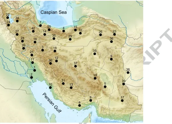
In this study, the monthly precipitation data of 40 synoptic weather stations located in Iran were analyzed. The study area, Iran, covers an area of about 1,648,000 km2, and lies between the latitudes 25° to 40° North and longitudes 44° to 64° East. The spatial distribution of the selected stations is fairly uniform across Iran. The selected stations have a record of 41 years covering the period from 1971 to 2011.
7
The two important mountain ranges of Iran are the Alborz and Zagros. Alborz, in located the northern part of Iran, extending along the southern Caspian Sea, while Zagros, is located in the western part of Iran, extending from the northwest to the southwest, impede Mediterranean moisture systems crossing through Iran (Shiau and Modarres, 2009). Most of the eastern part of the Iran is comprised of two great deserts called Dasht-e Kavir and Dasht-Dasht-e Loot (AbolvDasht-erdi and Khalili, 2010a). ThDasht-esDasht-e mountain rangDasht-es and deserts have a great influence on the spatial and temporal distribution of precipitation and temperature over Iran (Dinpashoh et al., 2004).
The map of the study area and the spatial distribution of the stations are illustrated in Fig. 1. Also, Table 1 presents the following attributes of the stations: names, geographical variables and mean of the annual precipitations. The data set was supplied by the Meteorological Organization of Iran.
3. Methodology
In this section, the methodology proposed for drought RFA is described. For this purpose, first, the steps of the analysis procedure are presented, and then the proposed approaches are given in the following subsections. The steps of the procedure are as follows:
1. Consider a number of sites within the region, and assemble the monthly precipitation data for each site,
2. Calculate the MSPI values and extract drought severities,
3. Determine the sub-regions by using the clustering method and cluster validity index,
8
4. Compute the heterogeneity and discordancy measures using L-moments approach,
5. Test the sub-regions for regional homogeneity, 6. Adjust the heterogeneous sub-regions, and 7. Specify the homogeneous sub-regions.
3.1. Multivariate Standardized Precipitation Index (MSPI)
Bazrafshan et al. (2014) recently developed the MSPI index for drought monitoring. The MSPI is based on the several time series of the Standardized Precipitation Index (SPI) and the Principal Component Analysis (PCA) as a multivariate approach. Unlike the MSPI index, the SPI index does not have the flexibility to consider a variety of time scales. So, this may result in a confusion in the identification of drought periods. On the other hand, relating a certain type of drought impact to the size of the time scale is still ambiguous. In this case, the PCA is utilized to aggregate a set of the SPI time series (i.e., the K original variables) into a new set of time series. Among these new variables, the first one (the first principal component, PC1) has a great percentage of variance of the K original variables. Because of the algebraic characteristic of PCA, the values of PC1 need to be standardized in proportion to the means and standard deviations of the different months of the year. Finally, the time sequence of the standardized values indicates the MSPI time series (Bazrafshan et al., 2014).
The MSPI can be computed for every selected set of the SPI time scales. In this study, twelve time scales from 1 to 12 months are considered as the input variables. The
9
selected time scales represent seasonal variations of precipitation throughout the year (Bazrafshan et al., 2015).
The MSPI time series can be calculated as follows
• Compute the SPI time series for the time scales set of 1-12 months, • Determine the first principal component series (PC1),
• Form the PC1ym matrix by subdividing the time series of the PC1 into 12 smaller series corresponding to 12 months (m) of year (y),
• Standardize the PC1ym as follows:
1 1 1 1 1 1 PC PC PC Z SD SD m ym ym ym m m − = ≈ (1)
where Z1ym is the standardized value of the PC1ym in the yth year and the mth month, and PC1m and SD1m are the mean and the standard deviation of PC1 in the mth month. Because of the negligible value of PC1m, it can be omitted in the above equation. • Determine the MSPI time series by reshaping the Z1ym matrix into one vector with
time sequence.
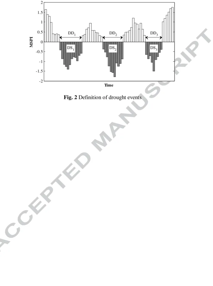
Two main drought characteristics, namely, severity and duration, can be derived based on the MSPI series. Drought duration (DD) is defined as the number of consecutive intervals (months) for which the MSPI values are less than zero. Drought severity (DS) is computed based on the absolute value of cumulative MSPI values within the drought duration (Abdi et al., 2016a).
The drought characterization such as duration and severity of the drought events and the time series of MSPI are illustrated in Fig. 2.
10
3.2. Growing Neural Gas (GNG) network
The main idea of the GNG network is to successively add new nodes (neurons) to an initially small network in a growing structure (Cirrincione et al., 2011). In the GNG, the network’s neurons compete to determine the ones with the highest similarity to the input data set (Morell et al., 2014).
The network is specified as (Fritzke 1995):
• A set of neurons. Each neuron c has its associated reference vector
w
c∈
R
d. The reference vector can be regarded as the neuron’s position in the input space.• A set of edges (connections) between pairs of neurons. These edges are used to define the topological structure.
The GNG algorithm can be summarized in the following steps (Fritzke 1995):
Step 1: Start with two neurons a and b at random positions wa and wb in the input space. Step 2: Present an input vector x from the training data set.
Step 3: Find the nearest neuron s1 and the second nearest neuron s2. Step 4: Increment the age of all edges emanating from s1 to its neighbors.
Step 5: Increase the local error of s1 by using the Euclidean distance between the two vectors as: 1 1 2 s s
E
w
x
∆
=
−
(2)Step 6: Move s1 and its direct topological neighbors towards x by learning rates εb and εn, respectively, of the total distance:
(
)
1 1 s b s w ε x w ∆ = − (3)(
)
n n n wε
x w ∆ = − (4)
11
where n represents all direct neighbors of s1.
Step 7: If s1 and s2 are connected by an edge, set the age of this edge to zero. If such an edge does not exist, create it.
Step 8: Remove edges with an age larger than amax. If this results in points having no emanating edges, remove them as well.
Step 9: If the number of input vectors presented so far is an integer multiple of a parameter λ, insert a new neuron as follows:
• Determine the neuron q with the largest error variable,
• Find the neuron f with the largest error variable among the neighbors of the neuron q,
• Insert a new neuron r halfway between q and f as wr =0.5
(
wq +wf)
• Create edges connecting the neuron r with neurons q and f, and remove the original edge between q and f, and
• Decrease the error variables of q and f by multiplying them with a fraction α. Set the error variable of r with the new value of the error variable of q.
Step 10: Decrease all error variables by multiplying them with a fraction β.
Step 11: If a stopping criteria (e.g., the maximum number of neurons or any performance measure) is not yet fulfilled go to step 2.
In summary, the age parameter considered in step 4 shows how strong the link between neurons is. In step 5, the neuron’s local error is used to identify areas where neurons are not sufficiently adapted to input vectors. The adaptation of the network to the input space takes place in step 6. The insertion of edges (step 7) between the two closest neurons to the input patterns is part of the topological structure construction process. The removal of
12
edges (step 8) is necessary to eliminate the edges between neurons that are no longer activated. In step 9, the new neuron is inserted in the areas of the input space by using the accumulated error (step 5). Finally, the network is continued until an ending condition is fulfilled (Cirrincione et al., 2011; Fišer et al., 2013; Morell et al., 2014; Quintana-Pacheco et al., 2014).
3.3. Minimum Description Length (MDL) measure
Rissanen (1989) originally proposed the MDL principle as a model selection criterion. The MDL can be applied for determining the optimum number of clusters by minimizing the length of description of the training data set (Rao and Srinivas, 2008). The data set X can be divided in two subsets I and O, which are composed of inliers and outliers, respectively. The expression of the MDL criterion is formulated according to the set of cluster centroids W as follows:
(
)
(
)
( )
MDL( ,X W)=modL I W, +errorL I W, +modL O (5)
where mod L(I,W), error L(I,W) and mod L(O) represent the complexity of the entire model, the residual errors generated by describing all inlier data points I with set W, and the description length of the outlier set, respectively (Rao and Srinivas, 2008).
The calculation of the MDL value can be instantiated by:
2 2
1 1
MDL( ,X W) log max log ,1 O
i c d k ik i x S k x w c K N c κ K η = ∈ = − = + +
∑ ∑ ∑
+ (6)where c, d, N, η, Si and |O| represent the current number of neurons, the dimension of input vectors, the number of data samples, the resolution of the data source, the receptive field of neuron wi and the cardinality of the outlier set, respectively. The value of K is
13
computed based on the average value range of the input vectors and the data accuracy η as K =[log (range2 η)]. Parameter κ is used to balance the contribution of model complexity and model efficiency (Qin and Suganthan, 2004).
The optimum number of clusters is determined by calculating the MDL values for a number of clusters (i.e., from 2 to 10) and saving the smallest value.
3.4. Discordancy and heterogeneity measures
Hosking (1986, 1990) proposed the L-moments as linear combinations of the probability weighted moments (PWM), which can be interpreted as measures of the location, scale, and shape of probability distributions. Based on the L-moments, Hosking and Wallis (1993) defined useful statistics in the RFA such as the discordancy and heterogeneity measures.
The discordancy measure (Di) is used to recognize discordant site(s) in a region. This measure for the ith site in a region is defined as:
(
)
T 1(
)
3 i i i N D = u −u S− u −u (7) 1 1 N i i u u N = =∑
(8)(
)(
)
1 N T i i i S u u u u = =∑
− − (9)where N is the number of sites, ui = [t(i), t3(i), t4(i)]T is a vector of the L-moment ratios for the ith site. The components of the vector ui are: t as the L-coefficient of variation (L-CV), t3 as the L-coefficient of skewness (L-CS) and t4 as the L-coefficient of kurtosis (L-CK), respectively. The regional unweighted average of vectors ui for all sites is denoted
14
u , and S is the matrix of sums of squares and cross-products. The critical discordancy measure is equal to 3 and the site becomes discordant when Di>3 (Hosking and Wallis, 1993; 1997).
The heterogeneity measure (Hi) is utilized to compute the degree of heterogeneity in a region. This measure can be computed as follows:
(
)
, 1, 2, 3i i v i vi
H = V −µ σ i= (10)
where Vi, µvi and σvi represent the V variables, the mean and the standard deviation of the simulated V variables, respectively. The V variables (Vi) for different values of i are given as: ( )
(
)
0.5 2 1 1 1 N N i R i i i i V n t t n = = = − ∑
∑
(11) ( )(
)
( )(
)
{
2 2}
0.5 2 3 3 1 1 N N i R i R i i i i V n t t t t n = = =∑
− + −∑
(12) ( )(
)
( )(
)
{
2 2}
0.5 3 3 3 4 4 1 1 N N i R i R i i i i V n t t t t n = = =∑
− + −∑
(13) where, ,
3 4 R R Rt t t
and ni are the regional L-moment ratios and the sample size for site i,respectively.
In order to compute the values of µvi and σvi, it is necessary to simulate the synthetic regions. For this purpose, the four-parameter Kappa distribution is fitted to the regional sample data. A large number (e.g., Nsim=1000) of synthetic regions are simulated by using the known parameters of the Kappa distribution. The simulated V variables are determined for each simulated region and then for these variables, the means (µv1, µv2 and µv3) and standard deviations (σv1, σv2 and σv3) are determined.
15
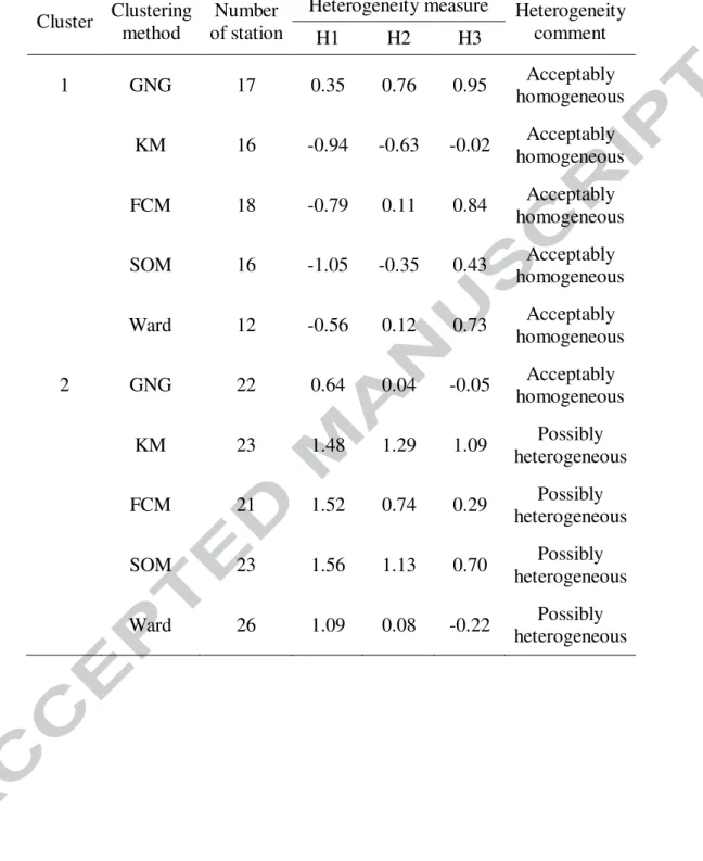
Hosking and Wallis (1993) suggested that a region is “acceptably homogeneous” if Hi is less than 1, “possibly heterogeneous” if Hi is between 1 and 2, and “definitely heterogeneous” if Hi is greater than 2.
4. Results
4.1. Drought characterization
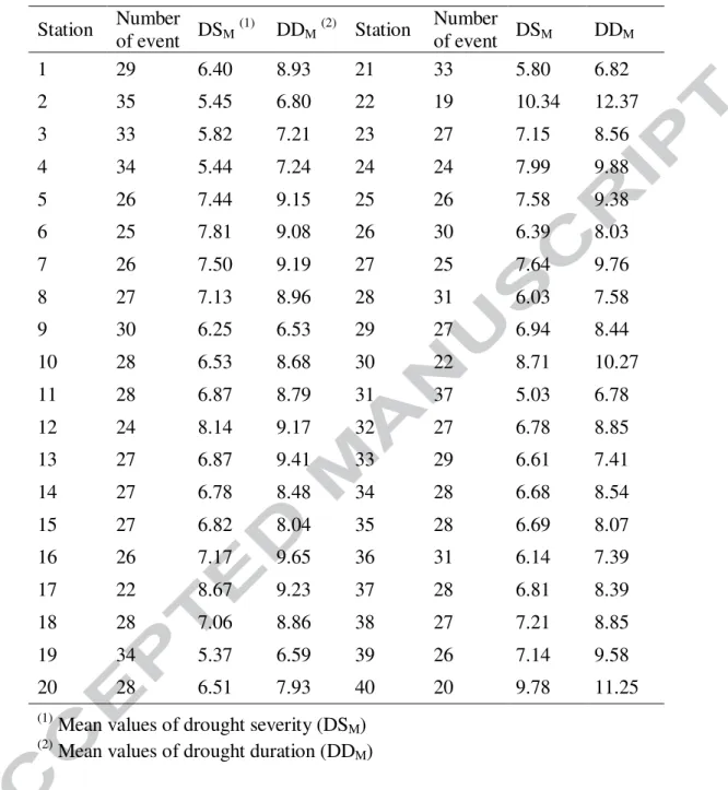
At first, the MSPI values are calculated using monthly precipitation data for all stations. According to the time series of the MSPI, the relative frequencies of three classes of drought, including moderate (−1.5<MSPI≤ −1.0), severe (−2.0<MSPI≤ −1.5), and extreme (MSPI≤ −2.0) in all stations are given in Table 2. This Table illustrates that the MSPI can identify the extreme drought class in all stations. Then, drought characteristics such as drought severity and drought duration are derived based on the MSPI time series. Table 3 shows, for a number of drought events at all stations in the study area, the mean values of drought severity (DSM) and drought duration (DDM).
4.2. Cluster Analysis
It is necessary to normalize the input data set before applying the clustering method. This is due to the fact that results can be affected by the different units of the variables, including drought severities and the geographical attributes of each station. Based on the rescaled data set, the sub-regions can be determined by using the clustering methods. For this purpose, the new GNG method and the conventional Ward, KM, FCM and SOM methods are utilized in this study.
16
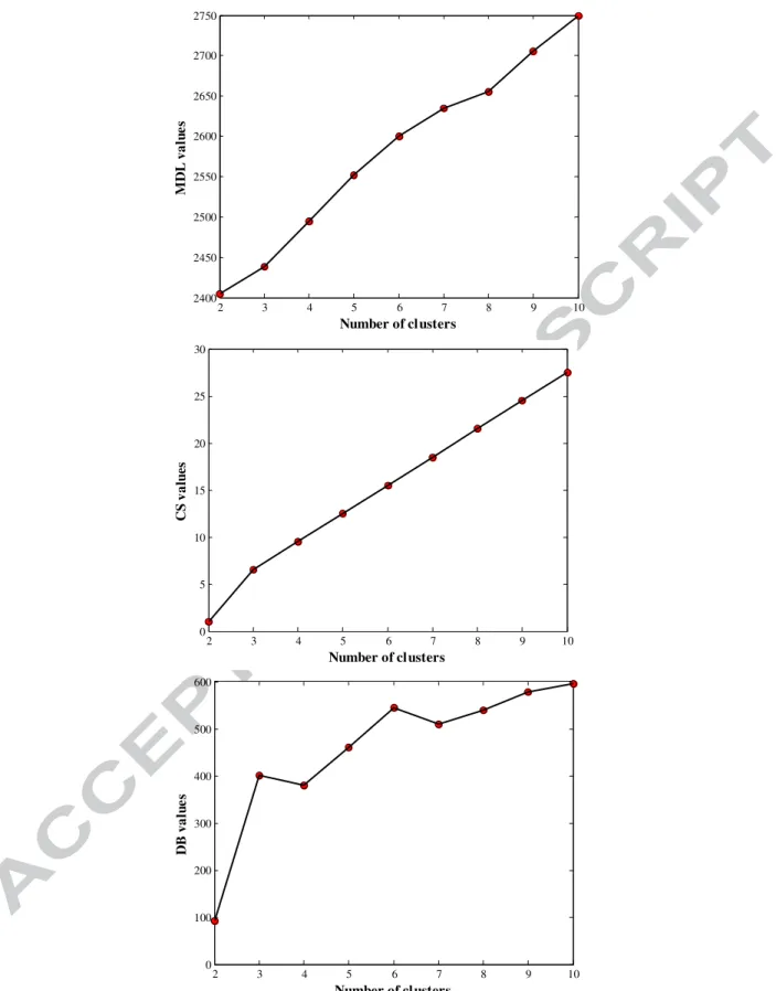
In order to find the optimum number of clusters (c), the MDL measure proposed for the GNG network and two different indices namely the CS index (Chou et al., 2004) and the Davies–Bouldin Index (DB; Davies and Bouldin, 1979) are used in the present study. Fig. 3 illustrates the values of the proposed indices for a number of clusters, by incrementally increasing c from 2 to 10. It can be seen from Fig. 3 that the optimum number of clusters is equal to two based on the minimum value for each of the three measures. In addition, the values of the MDL and the CS indices increase with the number of clusters.
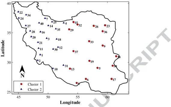
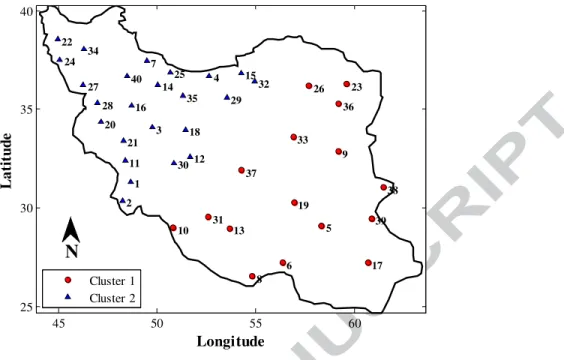
According to the value c=2 as the optimum number of clusters, the outputs of the clustering methods, namely GNG, KM, FCM, SOM and Ward, show that the study area is subdivided in two different sub-regions, located in the west and the east side of Iran. Figs. 4 to 8 illustrate the location of the stations in two different sub-regions identified by GNG, KM, FCM, SOM and Ward method, respectively. As it can be seen in the Figs. 4 to 8, the results of these methods are different in some stations, which refer to the mechanism of the used clustering algorithms. In addition, sub-region 1 represents the eastern side of Iran, and sub-region 2 covers the western side of Iran. These results confirm the details mentioned in the previous section about the physiographic features of the study area, in which the eastern and western parts of Iran are comprised of deserts and mountain ranges, respectively.
The parameters employed in the GNG algorithm are set as the typical values utilized in Daszykowski et al. (2002), Rêgo et al. (2010) and Fišer et al. (2013): εb=0.05, εn=0.0006, α=0.5, β=0.9995, λ=100 and amax=50. The parameters considered in the MDL
17
measure are chosen as: κ=1.3 and η=1×10⁻⁴. These parameters are constant during the training procedure.
4.3. Regional homogeneity tests
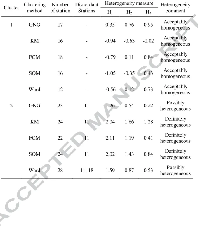
After the application of the clustering methods, the sub-regions are validated by testing their homogeneity through the obtained drought severities of the stations. In order to confirm the homogeneity of the sub-regions and to compare the efficiency of the clustering algorithms, the values of the heterogeneity measures and the identified discordant stations for each sub-regions are shown in Table 4. Results of the heterogeneity measures, which compare the L-moments of the observed and simulated data for the stations classified in two sub-regions, are different for all clustering methods. Therefore, Table 4 illustrates that sub-region 1 is ‘acceptably homogeneous’, whereas sub-region 2 is not homogeneous and needs adjustment. According to the results of Table 4, station 11 is identified as a discordant station for the GNG, KM, FCM and SOM methods, while stations 11 and 18 are discordant in sub-region 2 for the Ward method. Furthermore, the values of the heterogeneity measures for sub-region 2 show that the GNG and Ward methods yield a sub-region that is ‘possibly heterogeneous’, while the sub-region determined based on the KM, FCM and SOM methods is ‘definitely heterogeneous’.
In order to adjust sub-region 2 which is not ‘acceptably homogeneous’, the discordant stations can be removed. Table 5 illustrates the results of the heterogeneity measures after removing the discordant stations. According to Table 5, only the GNG algorithm yields an “acceptably homogeneous” sub-region 2 after removing the discordant stations.
18
Consequently, the GNG network is the best method for identifying the homogeneous two sub-regions with similar drought severities among several proposed clustering algorithms.
The main difference between the GNG network and the KM, FCM, SOM and Ward methods is the algorithm’s structure. Unlike the rigid structure of conventional methods, GNG has a dynamic structure, and while training, the nodes are moved over the input data space toward the optimal clusters. In addition, inserting new nodes and constructing or removing edges are applied to enhance the results of GNG algorithm. These approaches are important to find cluster members, especially for the members located near the boundary regions of multiple clusters (e.g., stations 10, 15, 29, 31 and 32). On the other hand, the GNG network has an ability to adapt its structure based on the statistical characteristics of the data set. As a result, the shape and size of the KM, FCM, SOM and Ward methods do not change over time. Therefore, these methods result in considerable limitations for the obtained groups.
5. Conclusions
In the present study, a new clustering technique, the Growing Neural Gas (GNG) network, is introduced to fields of hydrology and water resources, and employed more specifically in regional drought frequency analysis. For this purpose, the values of the Multivariate Standardized Precipitation Index (MSPI) were calculated using the monthly precipitation time series of 40 synoptic weather stations located in Iran. The drought severities derived from the MSPI time series and the geographical attributes of all stations were utilized in the GNG algorithm and various clustering methods, namely
19
means, fuzzy C-means, self-organizing map and Ward method. According to the Minimum Description Length (MDL) measure, the optimum number of sub-regions was found to be equal to two. Therefore, the outputs of the clustering algorithms considered in this study led to two different sub-regions, which are located in the eastern and western parts of Iran. Finally, by using the L-moments-based heterogeneity measure for testing the delineated sub-regions, the GNG algorithm was selected as the best clustering algorithm. The results of the present research effort pointed out to the dynamic and flexible structure of the GNG network, in contrast with the rigid structure of the conventional KM, FCM, SOM and Ward methods.
This study presented a first application of the GNG network for drought regionalization. This method can be applied for the regionalization of the other hydrological variables, such as precipitations, floods, and suspended sediments. Future research efforts can focus on these directions along with other directions in the field of water resources. For instance, the rational definition of classes is of interest in the qualitative seasonal forecasting of precipitations.
Future research can also focus on the combination of the GNG network approach with a number of regional estimation techniques to form a complete RFA procedure (delineation of homogeneous regions and estimation). The GNG approach can also be applied in a bivariate or multivariate framework. One regional estimation approach of special interest for combination with the GNG approach is the multivariate index flood or index-drought approach (see Chebana and Ouarda, 2009). The true potential of the GNG method can be assessed through its combination with other approaches and its application to real world complex regionalization problems. The flexibility of the GNG approach
20
should help it lead to improved results for a number of applications in the field of water resources planning and management.
References
Abdi, A., Hassanzadeh, Y., Talatahari, S., Fakheri-Fard, A., Mirabbasi, R., 2016a. Parameter estimation of copula functions using an optimization-based method. Theor. Appl. Climatol. doi: 10.1007/s00704-016-1757-2.
Abdi, A., Hassanzadeh, Y., Talatahari, S., Fakheri-Fard, A., Mirabbasi, R., 2016b. Regional bivariate modeling of droughts using L-comoments and copulas. Stoch. Environ. Res. Risk. Assess. doi: 10.1007/s00477-016-1222-x.
Abdi, A., Hassanzadeh, Y., Talatahari, S., Fakheri-Fard, A., Mirabbasi, R., 2016c. Regional drought frequency analysis using L-moments and adjusted charged system search. J. Hydroinform. doi: 10.2166/hydro.2016.228.
Abida, H., Ellouze, M., 2006. Hydrological delineation of homogeneous regions in Tunisia. Water Resour. Manag. 20, 961-977.
Abolverdi, J., Khalili, D., 2010a. Development of regional rainfall annual maxima for southwestern Iran by L-moments. Water. Resour. Manage. 24, 2501-2526.
Abolverdi, J., Khalili, D., 2010b. Probabilistic analysis of extreme regional meteorological droughts by L-moments in a semi-arid environment. Theor. Appl. Climatol. 102, 351-366.
Angelopoulou, A., Psarrou, A., Garcia-Rodriguez, J., Orts-Escolano, S., AzorinLopez, J., Revett, K., 2015. 3D reconstruction of medical images from slices automatically landmarked with growing neural models. Neurocomputing 150, 16-25.
21
Angelopoulou, A., Psarrou, A., Rodríguez, J.G., 2011. A growing neural gas algorithm with applications in hand modelling and tracking. Adv. Comput. Intell. 6692, 236-243.
Asong, Z.E., Khaliq, M.N., Wheater, H.S., 2015. Regionalization of precipitation characteristics in the Canadian Prairie Provinces using large-scale atmospheric covariates and geophysical attributes. Stoch. Env. Res. Risk Assess. 29, 875-892. Atiem, A., Harmancioglu, N.B., 2006. Assessment of regional floods using L-moments
approach: the case of the River Nile. Water Resour. Manag. 20, 723-747.
Awadallah, A.G., Yousry, M., 2012. Identifying homogeneous water quality regions in the Nile River using multivariate statistical analysis. Water Resour. Manag. 26, 2039-2055.
Aydogdu, M., Firat, M., 2015. Estimation of failure rate in water distribution network using fuzzy clustering and LS-SVM methods. Water Resour. Manag. 29(5), 1575-1590.
Basu, B., Srinivas, V.V., 2014. Regional flood frequency analysis using kernel-based fuzzy clustering approach. Water Resour. Res. 50(4), 3295-3316.
Bazrafshan J., Hejabi, S., Rahimi, J., 2014. Drought monitoring using the multivariate standardized precipitation index (MSPI). Water Resour. Manage. 28, 1045-1060. Bazrafshan, J., Nadi, M., Ghorbani, K., 2015. Comparison of empirical copula-based
joint deficit index (JDI) and multivariate standardized precipitation index (MSPI) for drought monitoring in Iran. Water Resour. Manage. 29, 2027-2044.
Bischof, H., Leonardis, A., Selb, A., 1999. MDL principle for robust vector quantization. Pattern Anal. Appl. 2(1), 59-72.
22
Botzheim, J., Kubota, N., 2012. Growing neural gas for information extraction in gesture recognition and reproduction of robot partners. In Proceedings of the 23rd International Symposium on Micro-NanoMechatronics and Human Science, Nagoya, Japan, Nov. 4-7, pp. 149-154.
Bougrain, L., Alexandre, F., 1999. Unsupervised connectionist clustering algorithms for a better supervised prediction: application to a radio communication problem. In Proceedings of the International Join Conference on Neural Networks. Washington, USA, Jul. 10-16, pp. 3451-3456.
Bouguelia, M.R., Belaïd, Y., Belaïd, A., 2015. Online unsupervised neural-gas learning method for infinite data streams, in: Fred, A., De Marsico, M., (Eds.), Pattern Recognition Applications and Methods, Advances in Intelligent Systems and Computing 318, Springer International Publishing, Switzerland, pp. 57-70.
Carlevarino, A., Martinotti, R., Metta, G., Sandini, G., 2000. An incremental growing neural network and its application to robot control. Proceeding of the International Joint Conference on Neural Networks, Como, Italy, Jul. 24-27, pp. 323-328.
Charron, C., Ouarda, T.B.M.J., 2015. Regional low-flow frequency analysis with a recession parameter from a non-linear reservoir model. J. Hydrol. 524, 468-475. Chebana, F., Ouarda, T.B.M.J., 2007. Multivariate L-moment homogeneity test, Water
Resour. Res. 43, W08406, doi: 10.1029/2006WR005639.
Chebana, F., Ouarda, T.B.M.J., 2009. Index flood–based multivariate regional frequency analysis, Water Resources Research., 45, W10435, doi: 10.1029/2008WR007490.
23
Chen, L.H., Lin, G.F., Hsu, C.W., 2011. Development of design hyetographs for ungauged sites using an approach combining PCA, SOM and Kriging methods. Water Resour. Manag. 25(8), 1995-2013.
Chiang, S.M., Tsay, T.K., Nix, S.J., 2002. Hydrologic regionalization of watersheds. I: methodology developement. J. Water Resour. Plan. Manage. 1(3), 3-11.
Chou, C.H., Su, M.C., Lai, E., 2004. A new cluster validity measure for and its application to image compression. Pattern Anal. Applic. 7, 205-220.
Cirrincione, M., Pucci, M., Vitale, G., 2011. Growing neural gas (GNG)-based maximum power point tracking for high-performance wind generator with an induction machine. IEEE Transactions on Industry Applications 47(2), 861-872.
Cirrincione, M., Pucci, M., Vitale, G., 2012. Growing neural gas-based MPPT of variable pitch wind generators with induction machines. IEEE Transactions on Industry Applications 48(3), 1006-1016.
Cretu, A.M., Petriu, E., Payeur, P., 2008. Evaluation of growing neural gas networks for selective 3D scanning. In Proceedings of the IEEE International Workshop on Robotic and Sensors Environments, Ottawa, Canada, Oct. 17-18, pp. 108-113.
Cselényi, Z., 2005. Mapping the dimensionality, density and topology of data: The growing adaptive neural gas. Comput. Meth. Programs Biomed. 78, 141-156.
Daszykowski, M., Walczak, B., Massart, D.L., 2002. On the optimal partitioning of data with K-means, growing K-means, neural gas, and growing neural gas. J. Chem. Inf. Comput. Sci. 42, 1378-1389.
Davies, D.L., Bouldin, D.W., 1979. A cluster separation measure. IEEE Trans. Pattern Anal. Mach. Intell. 1, 224-227.
24
Decker, R., 2005. Market basket analysis by means of a growing neural network. Int. Rev. Retail Distrib. Consum. Res. 15(2), 151-169.
Dikbas, F., Firat, M., Koc, A.C., Gungor, M., 2013. Defining homogeneous regions for streamflow processes in Turkey using a K-means clustering method. Arab. J. Sci. Eng. 38, 1313-1319.
Dikbas, F., Firat, M., Koc, A.C., Gungor, M., 2012. Classification of precipitation series using fuzzy cluster method. Int. J. Climatol. 32(10), 1596-1603.
Dinpashoh, Y., Fakheri-Fard, A., Moghaddam, M., Jahanbakhsh, S., Mirnia, M., 2004. Selection of variables for the purpose of regionalization of Iran’s precipitation climate using multivariate methods. J. Hydrol. 297, 109-123.
Donatti, G.S., Würtz, R.P., 2009. Using growing neural gas networks to represent visual object knowledge. In Proceedings of the 21st IEEE International Conference on Tools with Artificial Intelligence, IEEE Computer Society, Newark, USA, Nov. 2-4, pp. 54-58.
Ferrer, G. J. 2014. Creating visual reactive robot behaviors using growing neural gas. In Proceedings of the 25th Modern Artificial Intelligence and Cognitive Science Conference, Spokane, USA, Apr. 26, pp. 39-44.
Figueiredo, A.M., Gattass, M., Szenberg, F., 2007. Seismic horizon mapping across faults with growing neural gas. In Proceedings of the 10th International Congress of the Brazilian Geophysical Society. Rio de Janeiro, Brazil, Nov. 19-22, pp. 1476-1481. Fink, O., Zio, E., Weidmann, U., 2015. Novelty detection by multivariate kernel density
estimation and growing neural gas algorithm. Mech. Syst. Signal Proc. 50-51, 427-436.
25
Fišer, D., Faigl, J., Kulich, M., 2013. Growing neural gas efficiently. Neurocomputing 104, 72-82.
Fritzke, B., 1995. A growing neural gas network learns topologies, in: Tesauro, G., Touretzky, D.S., Leen, T.K., (Eds.), Advances in neural information processing systems. MIT Press, pp. 625-632.
García-Marín, A.P., Estévez, J., Medina-Cobo, M.T., Ayuso-Muñoz, J.L., 2015. Delimiting homogeneous regions using the multifractal properties of validated rainfall data series. J. Hydrol. 529, 106-119.
García-Rodríguez, J., Angelopoulou, A., García-Chamizo, J.M., Psarrou, A., Escolano, S.O., Giménez, V.M., 2012. Autonomous growing neural gas for applications with time constraint: optimal parameter estimation. Neural Netw. 32, 196-208.
García-Rodríguez, J., Flórez-Revuelta, F., García-Chamizo, J.M., 2007. Image compression using growing neural gas. In Proceedings of the International Joint Conference on Neural Networks, Orlando, USA, Aug. 12-17, pp. 366–370.
Gaume, E., Gaal, L., Viglione, A., Szolgay, J., Kohnova, S., Bloschl, G., 2010. Bayesian MCMC approach to regional flood frequency analyses involving extraordinary flood events at ungauged sites. J. Hydrol. 394, 101-117.
Goyal, M.K., Gupta, V., 2014. Identification of homogeneous rainfall regimes in northeast region of India using fuzzy cluster analysis. Water Resour. Manage. 28, 4491-4511.
Hailegeorgis, T.T., Thorolfsson, S.T., Alfredsen, K., 2013. Regional frequency analysis of extreme precipitation with consideration of uncertainties to update IDF curves for the city of Trondheim. J. Hydrol. 498, 305-318.
26
Hocking, A., Geach, J.E., Davey, N., Sun, Y., 2015. Teaching a machine to see: unsupervised image segmentation and categorisation using growing neural gas and hierarchical clustering. Instrum. Methods Astrophys. arXiv:1507.01589.
Hosking, J.R.M., 1986. The theory of probability weighted moments. Research Report RC12210, IBM Res. Div., Yorktown Heights, New York.
Hosking, J.R.M., 1990. L-moments: analysis and estimation of distributions using linear combinations of order statistics. J. R. Stat. Soc. Ser. B. 52(1), 105-124.
Hosking, J.R.M., Wallis, J.R., 1993. Some statistics useful in regional frequency analysis. Water Resour. Res. 29(2), 271-281.
Hosking, J.R.M., Wallis, J.R., 1997. Regional frequency analysis: an approach based on L-moments. Cambridge University Press, New York.
Ilorme, F., Griffis, V.W., 2013. A novel procedure for delineation of hydrologically homogeneous regions and the classification of ungauged sites for design flood estimation. J. Hydrol., 492, 151-162
Iyengar, R.N., Basak, P., 1994. Regionalization of Indian monsoon rainfall and long-term variability signals. Int. J. Climatol. 14(10), 1095-1114.
Jimeno-Morenilla, A., García-Rodríguez, J., Orts, S., Davia-Aracil, M., 2016. GNG based foot reconstruction for custom footwear manufacturing. Comput. Ind. 75, 116-126.
Jimeno-Morenilla, A., García-Rodriguez, J., Orts-Escolano, S., Davia-Aracil, M., 2013. 3D-based reconstruction using growing neural gas landmark: application to rapid prototyping in shoe last manufacturing. Int. J. Adv. Manuf. Technol. 69, 657-668.
27
Kahya, E., Demirel, M., Bég, O., 2008. Hydrologic homogeneous regions using monthly streamflow in Turkey. Earth Sci. Res. J. 12(2), 181-193.
Kar, A.K., Goel, N.K., Lohani, A.K., Roy, G.P., 2012. Application of clustering techniques using prioritized variables in regional flood frequency analysis - Case study of Mahanadi basin. J. Hydrol. Eng. 17(1), 213-223.
Kulkarni, A., 2016. Homogeneous clusters over India using probability density function of daily rainfall. Theor. Appl. Climatol. doi: 10.1007/s00704-016-1808-8.
Leclerc, M., Ouarda, T.B.M.J., 2007. Non-stationary regional flood frequency analysis at ungauged sites. J. Hydrol. 343, 254-265.
Lin, G.F., Chen, L.H., 2006. Identification of homogeneous regions for regional frequency analysis using the self-organizing map. J. Hydrol. 324, 1-9.
Linda, O., Manic, M., 2009. GNG-SVM framework - classifying large datasets with support vector machines using growing neural gas. In Proceedings of the International Joint Conference on Neural Networks, Atlanta, USA, Jun. 14-19, pp. 1820-1826.
Lisboa, P.J.G., Edisbury, B., Vellido, A., 2000. Business applications of neural networks: the state-of-the-art of real-world applications. World Scientific Publishing Company. Singapore.
Masselot, P., Chebana, F., Ouarda, T.B.M.J., 2016. Fast and direct nonparametric procedures in the L-moment homogeneity test. Stoch. Environ. Res. Risk. Assess. doi: 10.1007/s00477-016-1248-0.
Modarres, R., 2006. Regional precipitation climates of Iran. J. Hydrol. (New Zealand) 45(1), 13-27.
28
Modarres, R., 2010. Regional dry spells frequency analysis by L-moment and multivariate analysis. Water Resour. Manag. 24(10), 2365-2380.
Morell, V., Cazorla, M., Orts-Escolano, S., Garcia-Rodriguez, J., 2014. 3D Maps Representation Using GNG. Math. Probl. Eng. ID972304.
Ngongondo, C.S., Xu, C.Y., Tallaksen, L.M., Alemaw, B., Chirwa, T., 2011. Regional frequency analysis of rainfall extremes in Southern Malawi using the index rainfall and L-moments approaches. Stoch. Environ. Res. Risk Assess. 25, 939-955.
Nguyen, C.C., Gaume, E., Payrastre, O., 2014. Regional flood frequency analyses involving extraordinary flood events at ungauged sites: further developments and validations. J. Hydrol. 508, 385-396.
Noguera, J.V., Tortosa, L., Zamora, A., 2008. Analysis and efficiency of the GNG3D algorithm for mesh simplification. Appl. Math. Comput. 197, 29-40.
Núñez, J., Hallack-Alegría, M., Cadena, M., 2016. Resolving regional frequency analysis of precipitation at large and complex scales using a bottom-up approach: The Latin America and the Caribbean Drought Atlas. J. Hydrol. 538, 515-538.
Núñez, J.H., Verbist, K., Wallis, J.R., Schaefer, M.G., Morales, L., Cornelis, W.M., 2011. Regional frequency analysis for mapping drought events in north-central Chile. J. Hydrol. 405(3-4), 352-366.
Ogura, T., Iwasaki, V., Sato, C., 2003. Topology representing network enables highly accurate classification of protein images taken by cryo electron-microscope without masking. J. Struct. Biol. 143, 185-200.
29
Oliveira Martins, L., Silva, A.C., De Paiva, A.C., Gattass, M., 2009. Detection of breast masses in mammogram images using growing neural gas algorithm and ripley’s k function, J. Signal Process. Syst. 55(1-3), 77-90.
Orts-Escolano, S., Garcia-Rodriguez, J., Morell, V., Cazorla, M., Garcia-Chamizo, J.M., 2014. 3D colour object reconstruction based on growing neural gas. In Proceedings of the International Joint Conference on Neural Networks, Beijing, China, Jul. 6-11, pp. 1474-1481.
Ouarda, T.B.M.J., Girard, C., Cavadias, G.S., Bobée, B., 2001. Regional flood frequency estimation with canonical correlation analysis. J. Hydrol. 254(1–4): 157-173.
Ouarda, T.B.M.J., Ba, K.M., Diaz-Delgado, C., Carsteanu, A., Chockmani, K., GINGRAS, H., Quentin, E., Trujillo. E., Bobée B., 2008. Regional flood frequency estimation at ungauged sites in the Balsas River Basin, Mexico. J. Hydrol. 348: 40-58.
Qin, A.K., Suganthan, P.N., 2004. Robust growing neural gas algorithm with application in cluster analysis. Neural Netw. 17, 1135-1148.
Qin, A.K., Suganthan, P.N., 2005. Enhanced neural gas network for prototype-based clustering. Pattern Recognit. 38,1275-1288.
Quintana-Pacheco, Y., Ruiz-Fernández, D., Magrans-Rico, A., 2014. Growing neural gas approach for obtaining homogeneous maps by restricting the insertion of new nodes. Neural Netw. 54, 95-102.
Rahman, M.M., Sarkar, S., Najafi, M.R., Rai, R.K., 2013. Regional extreme rainfall mapping for Bangladesh using L-moment technique. J. Hydrol. Eng. 18(5), 603-615.
30
Rao, A.R., Srinivas, V.V., 2006a. Regionalization of watersheds by fuzzy cluster analysis. J. Hydrol. 318, 57-79.
Rao, A.R., Srinivas, V.V., 2006b. Regionalization of watersheds by hybrid-cluster analysis. J. Hydrol. 318, 37-56.
Rao, A.R., Srinivas, V.V., 2008. Regionalization of watersheds - An approach based on cluster analysis. Springer, New York.
Razavi, T., Coulibaly, P., 2013. Classification of Ontario watersheds based on physical attributes and streamflow series. J. Hydrol. 493, 81-94.
Rêgo, R.L.M.E.D., Araújo, A.F.R., Neto, F.B.D.L., 2010. Growing self-reconstruction maps, IEEE Trans. Neural Netw. 21, 211-223.
Rissanen, J., 1989. Stochastic complexity in statistical inquiry. Series in Computer Science, Vol. 15, World Scientific.
Santos, J.F., Portela, M.M., Pulido-Calvo, I., 2011. Regional frequency analysis of droughts in Portugal. Water Resour. Manag. 25, 3537-3558.
Satyanarayana, P., Srinivas, V.V., 2008. Regional frequency analysis of precipitation using large-scale atmospheric variables. J. Geophys. Res. Atmos. 113, D24110, doi: 10.1029/2008JD010412.
Satyanarayana, P., Srinivas, V.V., 2011. Regionalization of precipitation in data sparse areas using large scale atmospheric variables - A fuzzy clustering approach. J. Hydrol. 405, 462-473.
Shamshirband, S., Gocić, M., Petković, D., Javidnia, H., Ab Hamid S.H., Mansor, Z., Qasem, S.N., 2015. Clustering project management for drought regions determination: a case study in Serbia. Agric. For. Meteorol. 200, 57-65.
31
Shiau, J.T., Modarres, R. 2009. Copula-based drought severity-duration-frequency analysis in Iran. Meteorol. Appl. 16, 481-489.
Singh, K.K., Singh, S.V., 1996. Space time variation and regionalization of seasonal and monthly summer monsoon rainfall of the sub-Himalayan region and Gangetic plains of India. Clim. Res. 6, 251-262.
Srinivas, V.V., Tripathi, S., Rao, A.R., Govindaraju, R.S., 2008. Regional flood frequency analysis by combining self-organizing feature map and fuzzy clustering. J. Hydrol. 348, 148-166.
Steinbach, M., Ertoz, L., Kumar, V., 2003. The challenges of clustering high dimensional data, in: Wille, L.T., (Ed.), New directions in statistical physics - Econophysics, Bioinformatics, and Pattern Recognition, Springer, Germany, pp. 273-305.
Tenmoto, H., Kudo, M., Shimbo, M., 1998. MDL-based selection of the number of components in mixture models for pattern classification, in: Amin, A., Dori, D., Pudil, P., Freeman, H. (Eds.), Advance in Pattern Recognition: Lecture Notes in Computer Science 1451, Springer, pp. 831-836.
Viejo, D., Garcia, J., Cazorla, M., Gil, D., Johnsson, M., 2012. Using GNG to improve 3D feature extraction - Application to 6DoF egomotion. Neural Netw. 32, 138-146. Viglione, A., Laio, F., Claps, P., 2007. A comparison of homogeneity tests for regional
frequency analysis. Water Resour. Res. 43, W03428. doi: 10.1029/2006WR005095. Wallis, J., Schaefer, M., Barker, B., Taylor, G., 2007. Regional precipitation-frequency
analysis and spatial mapping for 24-hour and 2-hour durations for Washington States. Hydrol. Earth Syst. Sci. 11(1), 415-442.
32
Wazneh, H., Chebana, F., Ouarda, T.B.M.J., 2015. Delineation of homogeneous regions for regional frequency analysis using statistical depth function. J. Hydrol. 521, 232-244.
Yang, T., Shao, Q., Hao, Z.C., Chen, X., Zhang, Z., Xu, C.Y., Sun, L., 2010. Regional frequency analysis and spatio-temporal pattern characterization of rainfall extremes in the Pearl River Basin, China. J. Hydrol. 380, 386-405.
Yoo, J., Kwon, H.H., Kim, T.W., Ahn, J.H., 2012. Drought frequency analysis using cluster analysis and probability distribution. J. Hydrol. 420-421, 102-111.
Zaki, S.M., Yin, H., 2008. A semi-supervised learning algorithm for growing neural gas in face recognition. J. Math. Model. Algor. 7, 425-435.
Zhang, Q., Xiao, M., Singh, V.P., Li, J., 2012. Regionalization and spatial changing properties of droughts across the Pearl river basin, China. J. Hydrol. 472-473, 355-366.
33
List of Tables
Table 1 Attributes considered in this study Table 2 Relative frequencies of drought classes Table 3 Mean values of drought characteristics
Table 4 Results of heterogeneity measures before removing the discordant stations Table 5 Results of heterogeneity measures after removing the discordant stations
List of Figures
Fig. 1 Map of the study area with location of the stations Fig. 2 Definition of drought events
Fig. 3 MDL, CS and DB values versus the number of clusters Fig. 4 Location of stations in the sub-regions identified by GNG Fig. 5 Location of stations in the sub-regions identified by KM Fig. 6 Location of stations in the sub-regions identified by FCM Fig. 7 Location of stations in the sub-regions identified by SOM Fig. 8 Location of stations in the sub-regions identified by Ward
34
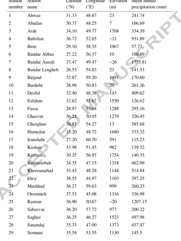
Table 1 Attributes considered in this study Station number Station name Latitude (°N) Longitude (°E) Elevation (m) Mean annual precipitation (mm) 1 Ahwaz 31.33 48.67 23 241.74 2 Abadan 30.37 48.25 7 166.69 3 Arak 34.10 49.77 1708 334.39 4 Babolsar 36.72 52.65 −21 931.89 5 Bam 29.10 58.35 1067 57.77 6 Bandar Abbas 27.22 56.37 10 180.89 7 Bandar Anzali 37.47 49.47 −26 1775.81 8 Bandar Lengheh 26.53 54.83 23 141.53 9 Birjand 32.87 59.20 1491 170.60 10 Bushehr 28.98 50.83 20 261.36 11 Dezful 32.40 48.38 143 409.62 12 Esfahan 32.62 51.67 1550 126.62 13 Fassa 28.97 53.68 1288 295.16 14 Ghazvin 36.25 50.05 1279 326.45 15 Ghorghan 36.85 54.27 13 585.68 16 Hamedan 35.20 48.72 1680 333.32 17 Iranshahr 27.20 60.70 591 115.23 18 Kashan 33.98 51.45 982 139.32 19 Kerman 30.25 56.97 1754 140.35 20 Kermanshah 34.35 47.15 1318 462.09 21 Khorramabad 33.43 48.28 1148 514.84 22 khoy 38.55 44.97 1103 297.25 23 Mashhad 36.27 59.63 999 260.23 24 Oroomieh 37.53 45.08 1316 336.98 25 Ramsar 36.90 50.67 −20 1207.15 26 Sabzevar 36.20 57.72 977 200.22 27 Saghez 36.25 46.27 1523 497.98 28 Sanandaj 35.33 47.00 1373 457.47 29 Semnan 35.58 53.55 1130 145.5
35 30 Shahrekord 32.28 50.85 2049 338.65 31 Shiraz 29.53 52.60 1484 329.76 32 Shahroud 36.42 54.95 1345 167.19 33 Tabass 33.60 56.92 711 86.01 34 Tabriz 38.08 46.28 1361 277.58 35 Tehran 35.68 51.32 1191 244.82 36 Torbate Heidarieh 35.27 59.22 1451 278.21 37 Yazd 31.90 54.28 1237 60.12 38 Zabol 31.03 61.48 489 59.07 39 Zahedan 29.47 60.88 1370 79.28 40 Zanjan 36.68 48.48 1663 307.59
36
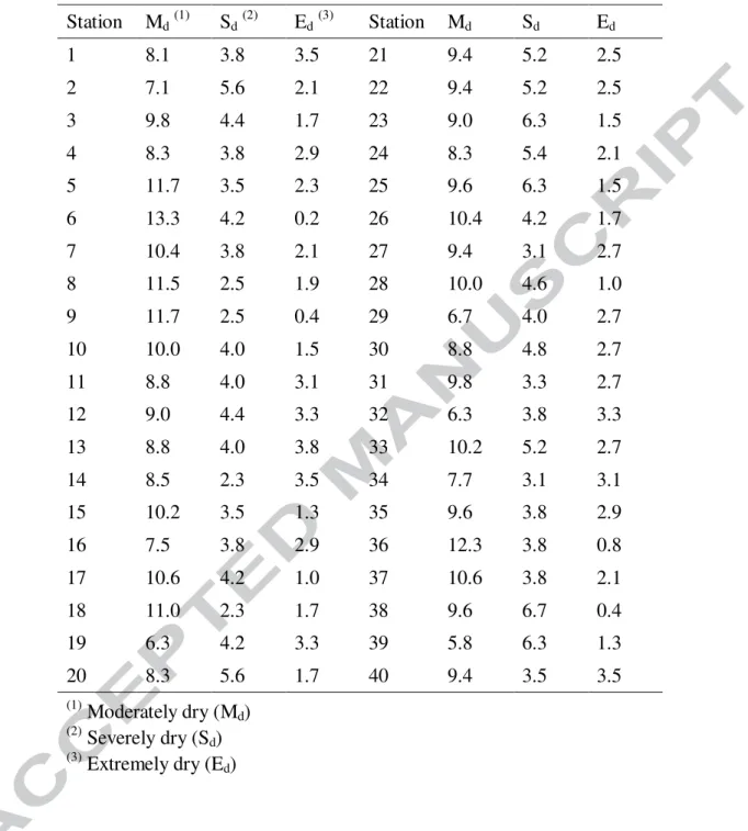
Table 2 Relative frequencies of drought classes
Station Md (1) Sd (2) Ed (3) Station Md Sd Ed 1 8.1 3.8 3.5 21 9.4 5.2 2.5 2 7.1 5.6 2.1 22 9.4 5.2 2.5 3 9.8 4.4 1.7 23 9.0 6.3 1.5 4 8.3 3.8 2.9 24 8.3 5.4 2.1 5 11.7 3.5 2.3 25 9.6 6.3 1.5 6 13.3 4.2 0.2 26 10.4 4.2 1.7 7 10.4 3.8 2.1 27 9.4 3.1 2.7 8 11.5 2.5 1.9 28 10.0 4.6 1.0 9 11.7 2.5 0.4 29 6.7 4.0 2.7 10 10.0 4.0 1.5 30 8.8 4.8 2.7 11 8.8 4.0 3.1 31 9.8 3.3 2.7 12 9.0 4.4 3.3 32 6.3 3.8 3.3 13 8.8 4.0 3.8 33 10.2 5.2 2.7 14 8.5 2.3 3.5 34 7.7 3.1 3.1 15 10.2 3.5 1.3 35 9.6 3.8 2.9 16 7.5 3.8 2.9 36 12.3 3.8 0.8 17 10.6 4.2 1.0 37 10.6 3.8 2.1 18 11.0 2.3 1.7 38 9.6 6.7 0.4 19 6.3 4.2 3.3 39 5.8 6.3 1.3 20 8.3 5.6 1.7 40 9.4 3.5 3.5 (1) Moderately dry (Md) (2) Severely dry (Sd) (3)
37
Table 3 Mean values of drought characteristics Station Number of event DSM (1) DDM (2) Station Number of event DSM DDM 1 29 6.40 8.93 21 33 5.80 6.82 2 35 5.45 6.80 22 19 10.34 12.37 3 33 5.82 7.21 23 27 7.15 8.56 4 34 5.44 7.24 24 24 7.99 9.88 5 26 7.44 9.15 25 26 7.58 9.38 6 25 7.81 9.08 26 30 6.39 8.03 7 26 7.50 9.19 27 25 7.64 9.76 8 27 7.13 8.96 28 31 6.03 7.58 9 30 6.25 6.53 29 27 6.94 8.44 10 28 6.53 8.68 30 22 8.71 10.27 11 28 6.87 8.79 31 37 5.03 6.78 12 24 8.14 9.17 32 27 6.78 8.85 13 27 6.87 9.41 33 29 6.61 7.41 14 27 6.78 8.48 34 28 6.68 8.54 15 27 6.82 8.04 35 28 6.69 8.07 16 26 7.17 9.65 36 31 6.14 7.39 17 22 8.67 9.23 37 28 6.81 8.39 18 28 7.06 8.86 38 27 7.21 8.85 19 34 5.37 6.59 39 26 7.14 9.58 20 28 6.51 7.93 40 20 9.78 11.25 (1)
Mean values of drought severity (DSM) (2)
38
Table 4 Results of heterogeneity measures before removing the discordant stations
Cluster Clustering method Number of station Discordant Stations
Heterogeneity measure Heterogeneity comment H1 H2 H3 1 GNG 17 - 0.35 0.76 0.95 Acceptably homogeneous KM 16 - -0.94 -0.63 -0.02 Acceptably homogeneous FCM 18 - -0.79 0.11 0.84 Acceptably homogeneous SOM 16 - -1.05 -0.35 0.43 Acceptably homogeneous Ward 12 - -0.56 0.12 0.73 Acceptably homogeneous 2 GNG 23 11 1.26 0.54 0.22 Possibly heterogeneous KM 24 11 2.04 1.66 1.28 Definitely heterogeneous FCM 22 11 2.11 1.19 0.41 Definitely heterogeneous SOM 24 11 2.02 1.43 0.84 Definitely heterogeneous Ward 28 11, 18 1.59 0.87 0.53 Possibly heterogeneous
39
Table 5 Results of heterogeneity measures after removing the discordant stations
Cluster Clustering method
Number of station
Heterogeneity measure Heterogeneity comment H1 H2 H3 1 GNG 17 0.35 0.76 0.95 Acceptably homogeneous KM 16 -0.94 -0.63 -0.02 Acceptably homogeneous FCM 18 -0.79 0.11 0.84 Acceptably homogeneous SOM 16 -1.05 -0.35 0.43 Acceptably homogeneous Ward 12 -0.56 0.12 0.73 Acceptably homogeneous 2 GNG 22 0.64 0.04 -0.05 Acceptably homogeneous KM 23 1.48 1.29 1.09 Possibly heterogeneous FCM 21 1.52 0.74 0.29 Possibly heterogeneous SOM 23 1.56 1.13 0.70 Possibly heterogeneous Ward 26 1.09 0.08 -0.22 Possibly heterogeneous
40
Fig. 1 Map of the study area with location of the stations 1 2 3 4 5 6 7 8 9 10 11 12 13 14 15 16 17 18 19 20 21 22 23 24 25 26 27 28 29 30 31 32 33 34 35 36 37 38 39 40 Caspian Sea
41
Fig. 2 Definition of drought events
-2 -1.5 -1 -0.5 0 0.5 1 1.5 2 Time M S P I DS 1 DS2 DS3 DD1 DD2 DD3
42
Fig. 3 MDL, CS and DB values versus the number of clusters
2 3 4 5 6 7 8 9 10 2400 2450 2500 2550 2600 2650 2700 2750 Number of clusters M D L v a lu e s 2 3 4 5 6 7 8 9 10 0 5 10 15 20 25 30 Number of clusters C S v a lu e s 2 3 4 5 6 7 8 9 10 0 100 200 300 400 500 600 Number of clusters D B v a lu e s
43
Fig. 4 Location of stations in the sub-regions identified by GNG
45 50 55 60 25 30 35 40 Longitude L a ti tu d e 1 2 3 4 5 6 7 8 9 10 11 12 13 14 15 16 17 18 19 20 21 22 23 24 25 26 27 28 29 30 31 32 33 34 35 36 37 38 39 40 Cluster 1 Cluster 2 N
44
Fig. 5 Location of stations in the sub-regions identified by KM
45 50 55 60 25 30 35 40 Longitude L a ti tu d e 1 2 3 4 5 6 7 8 9 10 11 12 13 14 15 16 17 18 19 20 21 22 23 24 25 26 27 28 29 30 31 32 33 34 35 36 37 38 39 40 Cluster 1 Cluster 2 N
45
Fig. 6 Location of stations in the sub-regions identified by FCM
45 50 55 60 25 30 35 40 Longitude L a ti tu d e 1 2 3 4 5 6 7 8 9 10 11 12 13 14 15 16 17 18 19 20 21 22 23 24 25 26 27 28 29 30 31 32 33 34 35 36 37 38 39 40 Cluster 1 Cluster 2 N
46
Fig. 7 Location of stations in the sub-regions identified by SOM
45 50 55 60 25 30 35 40 Longitude L a ti tu d e 1 2 3 4 5 6 7 8 9 10 11 12 13 14 15 16 17 18 19 20 21 22 23 24 25 26 27 28 29 30 31 32 33 34 35 36 37 38 39 40 Cluster 1 Cluster 2 N
47
Fig. 8 Location of stations in the sub-regions identified by Ward
45 50 55 60 25 30 35 40 Longitude L a ti tu d e 1 2 3 4 5 6 7 8 9 10 11 12 13 14 15 16 17 18 19 20 21 22 23 24 25 26 27 28 29 30 31 32 33 34 35 36 37 38 39 40 Cluster 1 Cluster 2 N
48