OATAO is an open access repository that collects the work of Toulouse
researchers and makes it freely available over the web where possible
Any correspondence concerning this service should be sent
to the repository administrator: [email protected]
This is an author’s version published in: http://oatao.univ-toulouse.fr/26929
To cite this version:
Soares Barbosa, Matheus Patrick and Rakotondrabe, Micky
and
Hultmann Ayala, Helon Vicente Deep learning applied to
data-driven dynamic characterization of hysteretic piezoelectric
micromanipulators. (2020) In: IFAC - WC, July 2020 (Berlin,
Germany).
Deep Learning Applied to Data-driven
Dynamic Characterization of Hysteretic
Piezoelectric Micromanipulators
Matheus Patrick Soares Barbosa∗Micky Rakotondrabe∗∗ Helon Vicente Hultmann Ayala∗
∗Dep. of Machanical Engineering, Pontifical Catholic University of
Rio de Janeiro, Brazil
(e-mails: [email protected], [email protected])
∗∗Laboratoire G´enie de Production, National School of Engineering in
Tarbes (ENIT-INPT), University of Toulouse, Tarbes France (e-mail: [email protected])
Abstract: The presence of nonlinearities such as hysteresis and creep increases the difficulty in the dynamic modeling and control of piezoelectric micromanipulators, in spite of the fact that the application of such devices requires high accuracy. Moreover, sensing in the microscale is expensive, making model feedback the only viable option. On the other hand, data-driven dynamic models are powerful tools within system identification that may be employed to construct models for a given plant. Recently, considerable effort has been devoted in extending the huge success of deep learning models to the identification of dynamic systems. In the present paper, we present the results of the successful application of deep learning based black-box models for characterizing the dynamic behavior of micromanipulators. The excitation signal is a multisine spanning the frequency band of interest and the selected model is validated with semi static individual sinusoidal curves. Various architectures are tested to achieve a reasonable result and we try to summarize the best approach for the fine tuning required for such application. The results indicate the usefulness and predictive power for deep learning based models in the field of system identification and in particular hysteresis modeling and compensation in micromanipulation applications.
Keywords: Identification and control methods; Micro and Nano Mechatronic Systems; Perception and sensing; Hysteresis modeling; Nonlinear system identification; Piezoeletric micromanipulators; Artificial neural networks
1. INTRODUCTION
System identification is the field within automatic control which encompasses the creation of dynamic models for the purposes of analysis and control of physical systems. Methods from system identification may be applied in a wide range of problems, also other than process control, such as biology in general [1], artificial pancreas [2], leg prosthesis [3], and water quality monitoring [4] to cite a few. Black-box modeling stands for the creation of mathematical abstractions of the system under study using solely input and output measurements. That is, no knowledge regarding the physical system is assumed to be available a priori and experiments are performed in order to enable the creation of the models offline. For its general applicability, nonlinear black-box modeling is an important tool for building models for different purposes such as simulation, analysis, and design.
Piezoeletric materials are recognized as actuators basis thanks to its high frequency rates, high resolution, porta-bility, and ease of intergration [5]. Moreover, in some situation, piezoelectric actuators might be used as their proper sensors allowing feedback control for performances
enhancement [6, 7, 8]. However, whenever actuating at the micro scale, sensing is not as easy to the uncertainties in the measured signals and to the difficulty to directly access. In such cases, it is mandatory to employ soft sensors to make possible the actuation using artificial feedback loops. In the literature we can find several methods for modeling such systems, e.g Preisach, Prandtl-Ishlinskii or Bouc-Wen models as noted in [9, 10, 11]. However, the precise modeling under those models require difficult and ad-hoc tuning which is a complex task in order to represent nonlinearities such as creep and hysteresis. As those characteristics are challenging in control design, the models used to tune the control laws should be equipped to better represent the actual system in simulation. As such, data-driven modeling such as black-box system identifica-tion is a general modeling framework which hinders the difficulties mentioned before.
In a previous work by the authors a 2-DOF piezoelectric actuator is modeled in [12], using shallow artificial neural networks at high frequency rates in a black-box approach. A piezo-actuated nanopositioning stage is controled in [13], where the effect of the applied voltage in the displacement is modeled locally as transfer. A multi axle piezo tube
is compensated in open-loop in [14], where the authors use a local linear model for inversion. In [15] the authors employ two coupled Hammerstein models to represent a 2-DOF piezocantilever in the task of micropositioning leveraged by an Kalman filter. Finally, [16] use MIMO transfer function to model other nonlinearities in multi-axes piezoelectric actuator and create an approximate inverse to their compensation.
Artificial neural networks have been long used for system identification [17] and have their roots tied with controls community. Radial basis functions [18] and multilayer per-ceptrons [19] are valuable tools for the nonlinear black-box system identification practitioner. On the other hand, deep learning has been given considerable attention from the research community and practitioners due to impressive improvements mainly in the field of image processing [20]. However, deep learning has not been extensively applied in system identification in order to solve complex dynamic systems modeling tasks. In [21] the authors use a restricted Boltzmann machine trained with random weights and test the methodology with standard benchmarks in system identification such as the gas furnace data [22], simulated nonlinear system [23] and the Wiener-Hammerstein case study [24]. In [25] the authors employ partial least squares regression in order to estimate deep neural models and evaluated the methodology with a simulated nonlinear system, a chaotic system, and the prediction of total phos-phorus quantity in a waste water treatment system with acquired data.
In this work we focus on the application of nonlinear black-box models to characterize the hysteretic behavior of piezoelectric micromanipulators using deep neural models as an alternative to the existing models. To this end, we perform specific data acquisition using a multipurpose signal for the estimation of model parameters that covers the whole frequency band of interest. Then we validate the created model with various individual sinusoidal input signals, in order to assert whether the hysteretic behav-ior has been adequately captured by the algorithm. The contributions of the paper thus are the following. We adapted and tested state-of-the-art deep neural networks Tensorflow c
framework [26] from Google in order to solve identification problems. These changes encompass the cre-ation of input/output pairs for estimcre-ation, validcre-ation and respective prediction horizon. Moreover, we confirmed that the general purpose multisine signal can be used for the creation of black-box models for micromanipulators, which is very convenient for the designer as the only parameters one has to tune is the frequency range, the sampling time, and the amplitude of interest. It is important to mention that all those parameters may be inferred for the task at hand. We also evaluated a series of deep neural network architectures, which may shed light for other researchers willing to apply the methods herein presented in problems which involve hysteresis which are frequently found in nature or of similar complexity.
The present paper is organized as follows. In Section II the methods employed in the present work related to nonlinear black-box system identification and signal excitation design are given. The case study is presented in Section III while in Section IV we give the results of the application of system identification to the problem of
hysteresis characterization in micromanipulators. Lastly, the conclusion and future works are stated in the last Section V.
2. NONLINEAR BLACK-BOX SYSTEM IDENTIFICATION
Nonlinear black-box system identification consists of build-ing mathematical abstractions of dynamic systems without (or with very little) any assumption about the physical properties of the system, relying purely on measured in-put and outin-put data [27]. It is a powerful and general framework for constructing data-driven dynamic models, with applications that span different fields.
Let u(t) and y(t) denote the input and output of the system at a given discrete-time instant t, and both these quantities are available. The NARX (Nonlinear AutoRe-gressive with eXogenous inputs) model is defined as
y(t) = F [y(t − 1), y(t − 2), . . . , y(t − ny),
u(t − 1), u(t − 2), . . . , u(t − nu)] + ξ(t);
(1) where ny and nu are the maximum lags (or orders of the
model) at the output and the input. The residual is defined as the error from the output of the model when compared to the measured output and can be calculated by
ξ(t) = y(t) − ˆy(t) (2)
where ˆy(t) is the predicted value. The function F [·] is a nonlinear function mapping in Rnφ → R from the
nφ model inputs to the model output. It describes the
dynamic relationship with past measured input and output data and thus describes the prediction of the model denoted by ˆy(t). The one-step-ahead (OSA) prediction is denoted by ˆy(t) as it is predicted based on most recent measurement. It differs from free-run simulation (FRS) from the fact that in the latter we use predictions over predictions to calculate the outputs of the model, which in many cases is more indicated to perform model validation as the errors accumulate over time.
2.1 Model Validation
We use error based metrics to evaluate the prediction accuracy of the models built. In order to do so, we employ multiple correlation coefficient (R2
) defined as [28, 29] R2= 1 − PN t=1[ξ(t)] 2 PN t=1[y(t) − ¯y] 2 (3)
where the upper bar denotes the mean value of the the sequence. The R2
shows in an uniform scale, without regard to the magnitude one is measuring, the prediction quality as its maximum value is one which implies all error sequences equal to zero.
It is important to mention that the R2
metric is calculated in OSA and FRS, for both the estimation and validation phases, but only the FRS were used to validate the model. 2.2 Excitation Signal
For the acquisition of input and output estimation data we may employ open loop experiments as the test bench
is available and no issues related to stability are expected. Thus we may design an ad-hoc excitation signal to perform the measurements. It is known that the exciting signal should span over the full band of interest and thus we employ the general purpose multisine excitation signal, for details on these issues see [30]. It may be calculated as
u(t) =
nf
X
k=1
Acos[2πfkt+ φk] (4)
where fk and φk are the frequency and phase components
of each sinusoidal components of the overall multisine signal. The total number of sinusoids should be large enough so that the frequency resolution is large enough. So each of fk may be determined equally spaced between
a minimum and maximum value of interest with nf
components. The phase, however, may be picked randomly in the range [0, 2π] for each component.
The excitation signals for the validation are pure sinu-soidals with the amplitude and frequency of interest. 2.3 Deep Learning Models
Deep neural models for regression may be described as ˆ
r= G[xxx, θθθ] (5)
where ˆris the predicted target value, xxxis the model input vector, θθθ is the set of weights which define the network, and G[·] is a nonlinear function mapping from the inputs of the network to the prediction. Following the notation in [31] we may further extend the definition in (5) as
ˆ r= φ X k wokφ X j wkjφ " . . . φ " X i wlixi ## (6)
where φ[·] is the neuron activation function, wok is the
synaptic weight from k−th to o−th layer. We can see from both definitions that the neural network is a concatenation of a single entity called neuron, which has different weights and biases throughout the structure.
The activation function φ[·] can be set as sigmoid, hyper-bolic tangent or rectified linear unit (ReLU), where z is the input. The latter is described as
φ(z) = max(0, z) (7)
where z is an input of a ReLU neuron and φ(.) is the activation function.
Once the architecture is defined, one should define the ob-jective function, or loss function, which will be minimized throughout the learning process. We define it as
L[xxx, θθθ; ppp] = 1 M M X i=1 [ri−rˆi] 2 (8) where M is the total amount of input/output pairs which amounts to the mean squared error (MSE). So by fine tuning the values in θθθ we expect to minimize the MSE and thus improve the predictive capability of the deep model. The neural models so defined are trained through an op-timization algorithm via stochastic gradient descent. Ac-cording to [32] the RMSprop training algorithm has been proposed by [33] and is among the most used options for finding the weights of deep neural networks architectures.
dSP A CE b oar d amplifier sensor piezocantilever (b) (a) sensor pie zo can tile v er
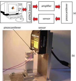
Fig. 1. Description of the piezoelectric actuator test bench. A voltage is applied to the active layer of the beam, which deflects due to the piezoelectric effect. (a) MATLAB and dSpace are used to send the input commands and store the data for identification which is performed offline. In (b) we show the real system where the acquisitions were made.
3. CASE STUDY: PIEZOELECTRIC MICROMANIPULATOR
The system studied in this paper consists of a piezoelec-tric actuator with cantilever structure with rectangular section and which is classically used in micromanipula-tion applicamicromanipula-tion. The actuator, exhibited in Fig. 1, has dimensions of (length, width, thickness): 15mm x 2mm x 0.3mm. When a voltage is applied to the piezoelectric actuator, it bends. This bending is exploited to push and to manipulate small objects [34]. The voltage (u), ranging between [-100V, 100V] is generated from a computer us-ing Matlab-Simulink and a High-Voltage-Amplifier (HVA). The bending (displacement y) of the actuator is measured with an optical displacement sensor having a resolution 10nm and a bandwidth of 5kHz: LK2420 from Keyence. Between the computer and the remaining elements of the setup (i.e. sensor, HVA amplifer, actuator), an acquisition board is used as converters: dS1104 from dSPACE. The acquisition board is set at 20kHz sampling frequency. This simple device exhibits nonetheless complex dynamic relation from the input voltage and deflection. This makes complicate its use in micropositioning applications, requir-ing sophisticated estimation and control loops to adhere to the problem requirements.
3.1 Measured Data
The data was acquired using the test bench previously described. We recorded two distinct datasets, (i) the multisine signal as in (4) and (ii) a pure sinusoidal signal for validation of the hysteresis modeling.
With respect to (i), the multisine was chosen because it is a general purpose excitation signal that can be designed
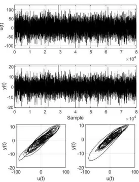
Fig. 2. Explorative plots of the measured input and output data. From top to below, we see the input [V] and output [µm] of the whole dataset with eight seconds (8e4 samples at 10 kHz). On the bottom we plotted five thousand samples from zero (left) and eight seconds (right) from the input and output relations.
to operate at a predefined frequency band. In Fig. 2 we depict the whole dataset for the estimation of the parameters of the model. It has been constructed with nf = 5000 sinusoidal signals and uniformly distributed
random phases, band of interest up to 0.5 kHz frequency and maximum amplitude of 100 V, as limited by the device.
The data was sampled at 10 kHz. We highlight that mod-eling in such high frequencies is important for rapid and accurate micropositioning. In Fig. 3 we show the power spectrum of the excitation signal and the output, spanning the band of interest up to 0.5 kHz. This band was chosen because it includes both the operation frequency range and the first resonant frequency of the piezo actuator. It is possible to see a peak around 800 Hz in the power spec-trum which is outside the excitation signal frequency band. Its presence may be due to non-linearities or unknown disturbances. We are not interested to analyse outside the excitation signal band and the amplitude of this peak is close to -40 dB, while the band of interest is at around 0 dB.
In (ii) we simply applied sinusoidal signals, one at a time, with different frequencies ranging from 0.1 Hz to 0.5 kHz. The pure sinusoidal signal frequently are used to evaluate the adherence of the model to capture the hysteretic behaviour, which is a major issue for the piezo cantilever in micropositioning tasks.
Fig. 3. Power spectrum for the multisine input and the measured output.
4. RESULTS
In the present section we depict the results obtained when applying deep neural nets for system identification of the piezoelectric micromanipulator. The input and output data for estimation data have been depicted in Subsection 3.1.
We have normalized all datasets and the results are given in dimensionless scale for sake of simplicity. This has been done to ease the learning process, as the inputs and outputs have different dimensions and this could make it more difficult as the optimization share the learning rate throughout the epochs.
We tested architectures with number of layers spanning from 3 to 5, where each layer is composed of 25, 50, or 100 neurons. We used also 100 epochs, learning rate 10−4,
a batch of 128 input/output pairs, and ReLU activation function. The order of models ny and nu were 10 and
the algorithm used to train the neural network was an RMSprop which divides the gradient by a running aver-age of its recent magnitude. The convergence of the loss and mean absolute error, during training phase, occurred during the first 25 epochs for most of the models, show-ing small improvements after the succeedshow-ing epochs. The choice of best model took in consideration the mean values of R2
obtained in the validation phase, the number of parameters and the complexity of architecture. In Table 1 it is possible to see all tested architectures and based on that, with 2501 total parameters, we choose the model with 4 layers of 25 neurons as it presents a better compro-mise between complexity and accuracy. In the following we depict the results of this model with respect to R2
obtained in the validation phase.
In Table 2 it is possible to see that all the values in the validation phase are close to unity. This shows the excellent prediction capability of the constructed models, as shown when performing FRS on a dataset that has a different nature than that of the estimation phase. Such quality improves our confidence on the model predictive capa-bility and encourages its use in soft sensor applications for example. The values obtained for R2
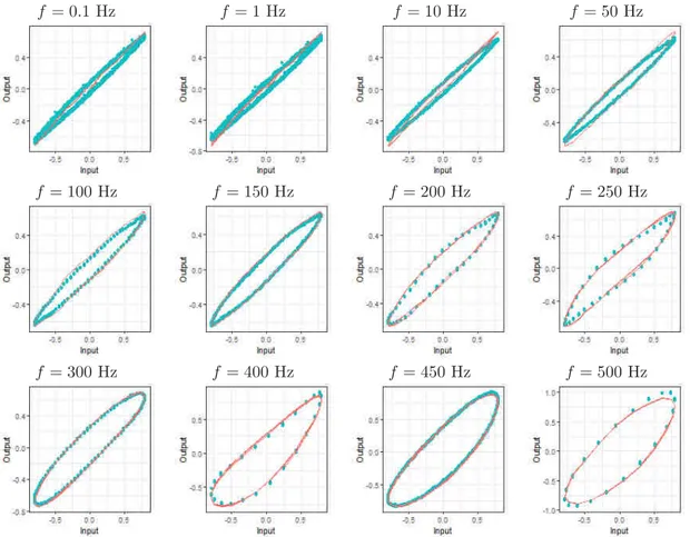
mentioned are confirmed in the plots illustrated in Fig. 4. We can see that the lines of prediction and measured data are virtually indistinguishable.
f = 0.1 Hz f = 1 Hz f = 10 Hz f = 50 Hz
f = 100 Hz f = 150 Hz f = 200 Hz f = 250 Hz
f = 300 Hz f = 400 Hz f = 450 Hz f = 500 Hz
Fig. 4. Output predictions for the selected model. Note that the data is normalized. Curves of u(t) versus y(t) (blue) and ˆys(t) (red) for the various frequencies tested in validation phase. Note that the hysteretic behavior has been
adequately captured for a wide band. Also, it is interesting to note how the hysteresis loop shape changes when the frequency increases.
Table 1. Mean of the values of R2
for all valida-tion datasets and total number of parameters, according to the different architectures tested.
Layers Neurons Mean R2 Parameters
3 25 0.984742017 1851 3 50 0.992217724 6201 3 100 0.964782331 22401 4 25 0.989210717 2501 4 50 0.916190505 8751 4 100 0.992844673 32501 5 25 0.992375649 3151 5 50 0.986898346 11301 5 100 0.992068821 42601 5. CONCLUSION
In the present paper we have successfully applied deep neural networks in the task of dynamic modeling of piezo-electric micromanipulators with real-world acquired data. We have created a dedicated general purpose excitation signal for acquiring data to create the model, giving indi-cation of the importance of multisine signals for hysteresis modeling as also remarked in [35] for a hysteretic simulated system. The importance of the steps given in this paper impacts compensator design and simulation, given the high accuracy of the model obtained.
Future research will be devoted to perform a full archi-tecture search and/or extensive hyper parameters tuning,
Table 2. Values for R2
in validation phase, varying frequencies for the excitation signal,
using 4 layers of 25 neurons.
Frequency (Hz) FRS 0.1 0.986797839 1 0.989170955 10 0.991136621 50 0.998469432 100 0.998403016 150 0.997474415 200 0.994559081 250 0.985648806 300 0.995859260 400 0.987992324 450 0.997331124 500 0.985664909
including, but not limited to, use of pyramid structure for the neural network, the automatic creation of the models using for that end neuroevolution techniques [36], which still lack relevant engineering applications that involve dynamic systems modeling such as monitoring, prediction, compensation, and simulation. It seems that the combina-tion of powerful complex representacombina-tion and ease of model creation may play an important role in the nonlinear black-box system identification space. Even if neuroevolution methods in the deep learning space imply greater com-putational burden, they are applicable in many
engineer-ing relevant situations and important for automatengineer-ing the model building activity which is time consuming and thus expensive to be made at scale, if not impossible, when problem dependent decisions are needed.
REFERENCES
[1] G. A. Bekey and J. E.W. Beneken. Identification of biological systems: a survey. Automatica, 14(1):41 – 47, 1978.
[2] I. Hajizadeh et al. Multivariable recursive subspace identification with application to artificial pancreas systems. IFAC WC, 50(1):886 – 891, 2017.
[3] M. Abdelhady et al. System identification and control optimization of an active prosthetic knee in swing phase. American Control Conf, pages 857–862, 2017. [4] M.B. Beck. In Hvdrological forecasting-Pr´evisions hydrologiques, volume 129 of Proceedings of the Ox-ford Symposium, pages 123–131. Int Association of Hydrological Science, April 1980.
[5] M. Rakotondrabe. Smart materials-based actuators at the micro/nano-scale. Characterization, Control and Applications. Springer, 2013.
[6] M. Rakotondrabe. Combining self-sensing with an unkown-input-observer to estimate the displacement, the force and the state in piezoelectric cantilevered actuator. American Control Conference, 2013. [7] O. Aljanaideh et al. Observer and robust h-inf control
of a 2-dof piezoelectric actuator equipped with self-measurement. IEEE Robotics Automation Letter, 3:1080-1087, 2018.
[8] I. A. Ivan et al. Quasi-static displacement self-sensing measurement for a 2-dof piezoelectric cantilevered ac-tuator. IEEE Transactions on Industrial Electronics, DOI.10.1109/TIE.2017.2677304, 2017.
[9] G-Y. Gu et al. Modeling and control of piezo-actuated nanopositioning stages: A survey. IEEE Trans on Automation Science and Eng, 13(1):313–332, 2014. [10] M. Rakotondrabe. Multivariable classical prandtl–
ishlinskii hysteresis modeling and compensation and sensorless control of a nonlinear 2-dof piezoactuator. Nonlinear Dynamics, 89(1):481–499, 2017.
[11] D. Habineza et al. Multivariable generalized bouc-wen modeling, identification and feedforward control and its application to a 2-dof piezoelectric multimorph actuator. IFAC WC, 10952-10958, 2014.
[12] H. V. H. Ayala, M. Rakotondrahe, and L. d. S. Coelho. Modeling of a 2-dof piezoelectric micromanipulator at high frequency rates through nonlinear black-box system identification. American Control Conference, pages 4354–4359, June 2018. [13] J. Ling et al. A robust resonant controller for
high-speed scanning of nanopositioners: Design and imple-mentation. IEEE Transactions on Control Systems Technology, 2019.
[14] D. Habineza et al. Multivariable compensation of hysteresis, creep, badly damped vibration, and cross couplings in multiaxes piezoelectric actuators. IEEE Transactions on Automation Science and Engineer-ing, 15(4):1639–1653, 2018.
[15] J. Escareno et al. Robust micro-positionnig control of a 2dof piezocantilever based on an extended-state lkf. Mechatronics, 58:82 – 92, 2019.
[16] M. Rakotondrabe. Modeling and compensation of multivariable creep in multi-dof piezoelectric actua-tors. IEEE ICRA, pages 4577–4581, 2012.
[17] K. S. Narendra and K. Parthasarathy. Identification and control of dynamical systems using neural net-works. IEEE Trans on Neural Networks, 1:4–27, 1990. [18] H. V. Hultmann Ayala and L. dos Santos Coelho. Cascaded evolutionary algorithm for nonlinear sys-tem identification based on correlation functions and radial basis functions neural networks. Mechanical Systems and Signal Processing, 68-69:378 – 393, 2016. [19] X. Li and W. Yu. Dynamic system identification via recurrent multilayer perceptrons. Information Sciences, 147(1):45 – 63, 2002.
[20] Y. LeCun, Y. Bengio, and G. Hinton. Deep learning. Nature, 521(7553):436, 2015.
[21] E. de la Rosa and W. Yu. Randomized algorithms for nonlinear system identification with deep learning modification. Information Sciences, 364, 2016. [22] G. E. P. Box and G. M. Jenkins. Time series analysis,
forecasting and control. Holden Day, San Francisco, USA, 1970.
[23] K. S. Narendra and K. Parthasarathy. Gradient methods for the optimization of dynamical systems containing neural networks. IEEE Transactions on Neural Networks, 2(2):252–262, March 1991.
[24] M. Schoukens and J.P. Noel. Three benchmarks addressing open challenges in nonlinear system iden-tification. IFAC WC, pages 446 – 451, 2017.
[25] J. Qiao et al. A deep belief network with PLSR for nonlinear system modeling. Neural Networks, 104:68– 79, 2018.
[26] T. Hope, Y. S. Resheff, and I. Lieder. Learning Ten-sorFlow: A Guide to Building Deep Learning Systems. O’Reilly Media, Inc., 1st edition, 2017.
[27] L. Ljung. Perspectives on system identification. An-nual Reviews in Control, 34(1):1 – 12, 2010.
[28] R Haber and H. Unbehauen. Structure identifica-tion of nonlinear dynamic systems–a survey on in-put/output approaches. Automatica, 26(4), 1990. [29] B. Schaible, H. Xie, and Y-C. Lee. Fuzzy logic models
for ranking process effects. IEEE Trans on Fuzzy Systems, 5(4):545–556, 1997.
[30] R. Pintelon and J. Schoukens. System identification: a frequency domain approach. John Wiley & Sons, Piscataway, NJ, 2 edition, 2012.
[31] S. S. Haykin. Neural networks and learning machines. Prentice Hall, Upper Saddle River, 3rd edition, 2009. [32] I. Goodfellow, Y. Bengio, and A. Courville. Deep
learning. MIT press, 2017.
[33] G. Hinton. Neural networks for machine learning, 2012.
[34] J.A Escareno, M. Rakotondrabe, and D. Habineza. Backstepping-based robust-adaptive control of a non-linear 2-dof piezoactuator. Control Engineering Prac-tice, 41:57–71, 2015.
[35] J.P. Noel, A.F. Esfahani, G. Kerschen, and J. Schoukens. A nonlinear state-space approach to hysteresis identification. Mechanical Systems and Sig-nal Processing, 84:171 – 184, 2017.
[36] K. O. Stanley, J. Clune, J. Lehman, and R. Miikku-lainen. Designing neural networks through neuroevo-lution. Nature Machine Intelligence, 1(1):24–35, 2019.