Thermal degradation of polymers during their mechanical recycling

Science Arts & Métiers (SAM)

is an open access repository that collects the work of Arts et Métiers Institute of Technology researchers and makes it freely available over the web where possible.

This is an author-deposited version published in: https://sam.ensam.eu Handle ID: .http://hdl.handle.net/10985/18678

To cite this version :

Xavier COLIN, Abbas TCHARKHTCHI - Thermal degradation of polymers during their mechanical recycling - 2013

Any correspondence concerning this service should be sent to the repository Administrator : archiveouverte@ensam.eu

T

HERMAL

D

EGRADATION OF

P

OLYMERS

DURING

T

HEIR

M

ECHANICAL

R

ECYCLING

Xavier Colin and Abbas Tcharkhtchi

ARTS ET METIERS ParisTech, PIMM (UMR CNRS 8006), Paris, France

A

This chapter deals with thermal degradation processes occurring during polymer recycling by melt re-processing, i.e. mechanical recycling.

Some general aspects of polymer processing are first recalled. Then, thermal degradation mechanisms and kinetics are described, and the main processing methods are compared from this point of view. Temperature–molar mass maps allow to define a processability window and to envisage industrial ways (in particular, the use of processing aids and thermal stabilizers) to widen this window. The end of this chapter is devoted to a case study: PET mechanical recycling by extrusion molding, which is characterized by an especially complex combination of degradation processes.

Keywords: Mechanical recycling, Melt processing, Processability window, Thermal

degradation, Kinetic modelling

I

The mechanical recycling of polymer wastes is the result of societal pressure to reduce environmental pollution, but also the willingness of industrialists to develop less expensive raw materials. Wastes are re-used after separation, grinding, washing and drying for the production of new polymer parts by melt re-processing (Scheirs 1998). One of the main sources of problems in polymer processing comes from their high melt viscosity (Van Krevelen and Te Nijenhuis 2009a). Indeed, the consumption of mechanical energy and the cost of tools (for instance, injection molds) could be significantly lowered and the productivity would be considerably increased if the melt viscosity was decreased by one (or several) order(s) of magnitude. As an indication, most of the industrial thermoplastic

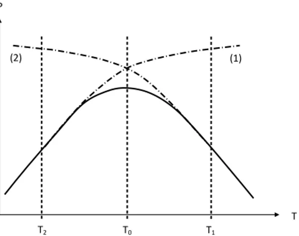
polymers are processed in the 400–650 K temperature range (Agassant et al. 1996). It is clear that processing in the 800–1000 K interval, where melt viscosity is expected to be typically 10–1000 times lower, would minimize the greater part of technological and economic constraints. Unfortunately, polymers are thermally instable at such high temperatures (Van Krevelen and Te Nijenhuis 2009b). Processing operations are thus performed in lower temperature ranges, where the melt viscosity is relatively high, just below what is called the thermal stability ceiling. But, this latter is a diffuse boundary: there is no discrete threshold for degradation processes. That is the reason why the optimum processing conditions involve generally a small sacrifice of the structural integrity of macromolecules, as schematized in Figure 1. If, in first approach, one considers constant the time necessary for a processing operation, one can determine two important temperature boundaries:

- At low temperature (T < T2), thermal degradation is negligible, but defects due to

high melt viscosity are responsible for the low quality of polymer parts. In this temperature range, mechano-chemical degradation processes can also occur.

- In contrast, at high temperature (T > T1), the part quality is essentially limited by

thermal ageing. Thermal degradation can affect processing properties through, essentially, polymer molar mass changes, but these effects are in general negligible during a single processing operation. However, the corresponding structural changes can be revealed after several successive re-processing operations (Assadi et al. 2004, Nait-Ali et al. 2011), and thus, affect, at more or less long-term, the use properties of the parts produced from recycled polymers (Table 1).

The processability window of a given polymer would correspond to these optimum processing conditions. The aim of the present chapter is to make a general analysis of polymer degradation processes during their melt processing, starting from the basic principles of polymer physics and thermal degradation mechanisms and kinetics. Temperature–molar mass maps will be used to define a processability window and to envisage industrial ways to widen this window. Then, the case of PET mechanical recycling by extrusion molding will be examined in details to illustrate the high complexity of the problem.

(1) (2)

P

T

T2 T0 T1

Figure 1. Schematization of the effects of the processing temperature on a property of industrial interest. The time spent for the processing operation is assumed constant. (1) Effect of physical parameters. (2) Effect of thermal degradation.

Table 1. Main types of structural changes occurring during polymer processing in liquid state. Consequences on main use properties.

1. T

A

M

P

G

A

1.1. Isothermal Ageing Characteristics

Let us consider a property P of industrial interest. Let us note PF its threshold value

required for the application under consideration. When the polymer undergoes an isothermal ageing at a given temperature T, a thermal degradation process occurs and leads to a change in P. One can define a conversion ratio x for this degradation process:

F 0 F t

P

P

P

P

x







where P0 and Pt are the respective property values at the beginning and after a duration t of

exposure. The degradation process is completed (x =0) when P = PF.

At this temperature, one can thus establish an aging function:

)

t

(

f

x



and determine the lifetime tF such as:

)

0

(

f

t



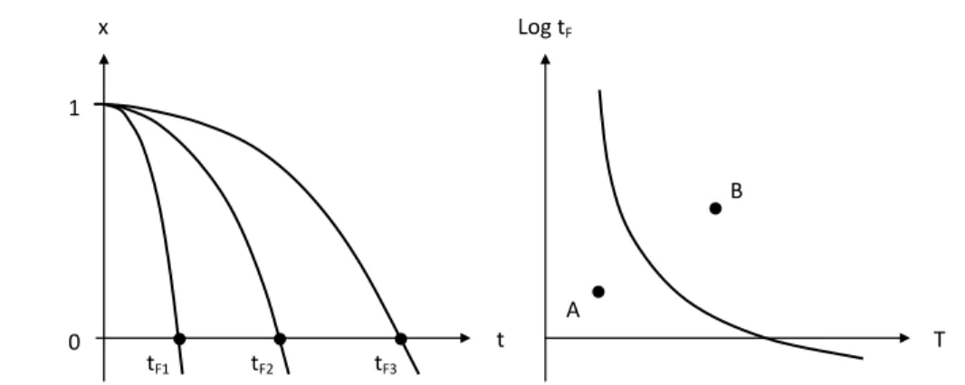
where f-1 is the reciprocal function of f. This last equation means that: x = 0 when t = tF. As

Log tF x t T B A tF1 tF2 tF3 0 1

Figure 2. Left: Principle of lifetime determination in kinetic degradation curves. Right: Shape of the temperature dependence of lifetime.

The history of a given polymer sample, used in given conditions, can be represented by a point in the timetemperature space (Figure 2, right). Its position relatively to the curve tF = f(t) gives immediately an information on its probable further evolution: If the point (for

instance A) is below the curve, this means that the material disposes of a residual lifetime. If, in contrast, the point is above the curve (for instance B), this means that the probability of failure is close to unity. Since the 40’s (Dakin 1948), it has been generally assumed that the thermal stability ceiling can be represented by a simple Arrhenius equation:











RT

H

exp

t

t

There are, however, many reasons to suppose that Arrhenius equation is, in many cases, inadequate to represent lifetime variations in a wide temperature range. Very powerful models, directly derived from mechanistic schemes and free of simplifying hypotheses, are now available thanks to the existence of efficient numeric computing tools, as shown, for instance, in the case of PE pipes transporting drinking water disinfected by chlorine reagents (Colin et al. 2009a and 2009b).

Even the problem of polymers stabilized by a synergetic blend of antioxidants is not insuperable (MKacher 2012).

1.2. Non-Isothermal Static or Dynamic Ageing

A processing machine can be considered as a chemical reactor displaying non-uniform temperature and shear fields. A first complication appears immediately: degradation occurs in a non-isothermal regime. The distribution of residence times in the machine (Pinto and Tadmor 1970), especially the existence of stagnation zones, must be taken into account. Another complication can come from the eventual role of shearing. First, it can play a role similar to stirring in (molecular) liquid reactors, favoring thus the homogenization of the reaction medium that can be important, for instance, in the case of stabilizers with low diffusivity.

Figure 3. Above: Temperature history. The whole processing time tw is the time spent above ambient

temperature (Tamb). te is the time spent by the polymer in liquid state. For a semi-crystalline polymer, Tm

and Tc are the melting point and the crystallization temperature respectively. For an amorphous

polymer, Tm and Tc are replaced by the glass transition temperature Tg. Below: Corresponding

degradation index for the polymer. xe corresponds to final degradation index at the end of the

processing operation.

The difference between “static” (no shear) and “dynamic” thermal ageing are well documented in the literature of the 60’s and 70’s. Shearing can also induce mechano-chemical chain scissions of which the main characteristic is to be disfavored by a temperature increase (Casale and Porter 1978). In the following, it will be considered that ageing tests are performed in conditions representative of processing ones.

Let us now return to the problem of non-isothermal ageing. Our reasoning will be based on the use of graphs in which the polymer history, during a given processing operation, is represented by a single temperature value Te which can be defined as follows.

The degradation process under consideration is characterized by the time te spent by the

polymer in liquid state. It is also characterized by the final degradation index xe of the

polymer at the end of the processing operation. Te is defined as the temperature of an

isothermal test which would lead to the same degradation index xe after the exposure time te.

In other words, Te is the temperature of an isothermal exposure equivalent to the temperature

history for the processing conditions under study. The determination of Te can be illustrated

by the simple example of a zero-order degradation process obeying an Arrhenius law:

r

dt

dx



with











RT

H

exp

r

r

T



f

(

t

)

)

t

(

F

r

dt

)

t

(

f

R

H

exp

r

dt

r

x

_



















_

_

where tw is the whole processing time and F(tw) the primitive function of

exp





H

R

f

(

t

)



According to the chosen definition of Te, one can write:

e e 0 e

t

T

R

H

exp

r

x

_



































t

/

)

t

(

F

Ln

R

H

T



Let us consider a temperature history T = f(t) for a given processing operation. It is characterized by its whole duration tw in the processing machine and the time te spent by the

polymer in liquid state (Figure 3).

1.3. The Problem of Small Conversions

Let us now consider the three main practical consequences of polymer thermal degradation during melt processing: changes in rheological property, embrittlement in solid state, and color change (for instance, yellowing).

The changes in rheological property result essentially from macromolecular modifications (i.e. changes in molar mass). In the case of a predominant random chain scission process, the number n of chain scissions is:





































1

M

M

p

p

M

1

1

M

M

p

p

M

p

M

p

M

p

n

where p, p0, Mw, Mw0, Mn and Mn0 are the respective values of polydispersity index and

weight and number average molar masses after and before ageing.

The change in Newtonian viscosity is linked to the change in molar mass by a well-known power law:

4 . 3 W 0 W 0

M

M























































1

p

p

M

1

n

At low conversion of the degradation process, p/p0 is of the order of unity. Thus, the

number of chain scissions necessary to divide the Newtonian viscosity by a factor 2 is of the order of: 0 n

M

2

.

0

n



i.e. for most of industrial polymers:

n  10-2 mol.kg-1 (15)

Crosslinking affects also rheological properties: gelation occurs when the number of crosslinks becomes equal to the number of weight average chains:

0 W

M

1

n



i.e. in general when:

n  2  10-2 mol.kg-1 (17)

Indeed, noticeable changes of the rheological behavior will appear far from the gelation point. Yellowing results generally from the formation of conjugated polyenes (in vinyl polymers) or oxidation products of aromatic rings, such as quinones or polyphenols (in aromatic polymers). The eye sensitivity to such structural changes depends on many parameters: initial color, presence of pigments, mode of sample illumination, sample thickness, etc. But, it is generally very high because chromophoric species have often a high absorptivity ( > 104 l.mol-1.cm-1 for most of the chemical species mentioned above) or a high emissivity, in particular when the color change is linked to luminescence as in the case of aromatic species. For initially white samples, at least, very small spectral changes can be easily detected visually. Even if, in most of cases, chromophore concentrations are less than 10-3 mol.kg-1, i.e. almost undetectable by classical spectrochemical techniques (such as FTIR and NMR), they can be the source of noticeable industrial troubles. Hydroperoxides resulting from thermal oxidation during melt processing play a key initiating role in further thermal or photochemical ageing in current use conditions. They can significantly affect the durability of

polymer parts. In the case of thermal oxidation, in the absence of antioxidants, a critical value of hydroperoxide concentration is:





k

k

POOH



where k1u and k1b are the respective rate constants of the uni- and bi-molecular decomposition

of POOH. As an example, [POOH]c 4  10 -2

mol.kg-1 for PE at 500 K (Colin et al. 2003). In the presence of preventive antioxidants (for instance, organic phosphites or sulfides), of which the usual concentration ranges between 10-3 and 10-2 mol.kg-1 in polyolefins, it is generally assumed that each hydroperoxide decomposition event leads to the consumption of one or two antioxidant molecules. From this brief literature survey, it can be concluded that small structural changes are sufficient to induce significant changes in use properties, in particular in rheological, mechanical, optical and durability properties. Studies in this field are thus confronted to analytical difficulties relative to the measurement of small chemical species concentrations. As an example, it is well known that PET hydrolysis cannot be monitored by routine FTIR or NMR measurements. Moreover, PP oxidation leads to embrittlement before any detectable change in IR spectra (Fayolle et al. 2008), despite the relative high sensitivity of FTIR titration of carbonyl groups. Finally, color change can appear in PVC well before that chromophoric species are detected by IR or NMR spectrophotometry.

2. T

O

2.1. Mechanistic Scheme

Thermal oxidation displays two very important features:

- It is a radical chain process propagated by abstraction of hydrogen atoms:

(II) P° + O2 → PO2° (k2)

(III) PO2° + PH → POOH + P° (k3)

where PH designate a CH bond, POOH an hydroperoxide group, and P° and PO2° alkyl and

peroxy radicals respectively. k2 and k3 are the rate constants of the elementary reactions under

consideration.The first step is very fast and practically temperature and structure independent: k2 = 10

8_

109 l.mol-1.s-1 for all polymers (Kamiya and Niki 1978). At the opposite, the second step is noticeably slower: it is even slower than the dissociation energy ED of the CH bond is

higher. Structure/k3 relationships have been investigated by Korcek et al. (1972). According

to these authors, Log(k3) would be a linear function of ED. As a piece of information, the

Arrhenius parameters and orders of magnitude at 30°C of the rate constant k3 have been

been compiled from previous research works performed in our laboratory (Colin et al. 2004, Colin et al. 2007, Sarrabi et al. 2008, Nait-Ali et al. 2011, El-Mazry et al. 2013).

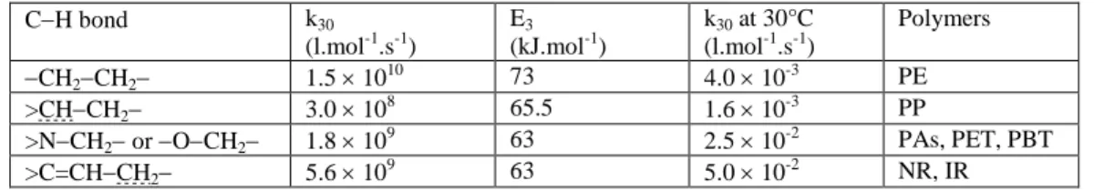
Table 2. Arrhenius parameters and orders of magnitude at 30°C of rate constant k3 for common methylenic and methynic CH bonds (Colin et al. 2004, Colin et al. 2007, Sarrabi et al. 2008, Nait-Ali et al. 2011, El-Mazry et al. 2013). Allylic and methynic CH

bonds are underlined

CH bond k30 (l.mol-1.s-1) E3 (kJ.mol-1) k30 at 30°C (l.mol-1.s-1) Polymers CH2CH2 1.5  1010 73 4.0  10-3 PE >CHCH2 3.0  108 65.5 1.6  10-3 PP >NCH2 or OCH2 1.8  10 9 ₆₃ 2.5  10-2 PAs, PET, PBT >C=CHCH2 5.6  109 63 5.0  10-2 NR, IR

Table 3. Orders of magnitude of the dissociation energy (ED) of main polymer chemical bonds

Chemical bond ED (kJ.mol-1)

aromatic C−C 510 C−F 470 aromatic C−H 465 aliphatic C−H 325−425 aliphatic C−C 300−380 C−O 340 C−Cl 320 C−Si 300 C−N 290 C−S 275 S−S 260 O−O 150

- Hydroperoxides resulting from propagation are highly unstable. Indeed, the dissociation energy of the OO bond is about 150 kJ.mol-1 against more than 250 kJ.mol-1 for all other polymer chemical bonds (Table 3).

The decomposition of hydroperoxides generates radicals:

(Iu) POOH → PO° + °OH (

G



G



-1

at 100°C)

where PO° and HO° designate alkoxy and hydroxy radicals respectively. Both free energy values can be compared to the CC scission one: (Ip) PP → 2P° (

G



All these features explain well the main characteristics of thermal oxidation processes:

a) They produce their own initiator: POOH. Because of this “closed-loop” character, oxidation starts with a very low rate, but displays an auto-accelerated behavior linked to hydroperoxide accumulation. Hydroperoxide decomposition (Iu or Ib) is expected to largely predominate over polymer decomposition (Ip) at low temperature. The Arrhenius plot of lifetime is expected to present the shape of Figure 4.

Below a certain temperature TA, depending on the polymer nature and sample thickness,

oxidation is always faster than decomposition in neutral atmosphere and displays always a lower activation energy. Let us recall that a fast and intense shearing of the molten polymer can induce mechano-chemical processes, i.e. mechanically activated reactions (Ip), which can participate to the initiation of oxidation radical chains and thus, tend to suppress the “closed-loop” character.

b) It is possible to envisage efficient ways of stabilization by introducing additives in low concentration in the molten polymer, in particular adequately chosen antioxidant molecules. There are two main types of such antioxidants:

 Preventive antioxidants, such as organic phosphites or sulfides, which reduce the initiation rate by decomposing the hydroperoxides by a non-radical way. Phosphites are generally considered as good melt processing antioxidants, even if they are not efficient against mechano-chemical reactions. In contrast, sulfides are rather efficient at lower temperature in current use conditions.

 Chain breaking antioxidants, such as hindered phenols or secondary aromatic amines, which increase the termination rate by scavenging radicals.

In practice, both types of antioxidants are associated in order to constitute synergistic blends of antioxidants. The most usual mixtures are: (phosphite + phenol) or (sulfide + phenol), plus, sometimes, a third component (a metal deactivator) aimed to prevent the eventual catalytic effects of metal impurities.

(O) (N)

Log tF

T-1 TA-1

Figure 4. Schematic shape of the Arrhenius plot of lifetime tF in the presence (O) and absence of

Table 4. Orders of magnitude of the dissociation energy (ED) of main polymer CH bonds. Allylic CH bonds are underlined

CH bond ED (kJ.mol-1) 465 CH3 414 CH2CH2 393 >CH 380 >NCH2 or OCH2 376 >C=CHCH2 335

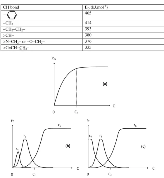
Figure 5. Effect of oxygen concentration C on global oxidation rate rox (a) and termination rates rT

without (b) and with (c) reaction (Ip).

c) The propagation rate depends essentially on the strength of the CH bond (Table 4). This order corresponds well to the observed hierarchy of polymer stabilities: polymers containing only aromatic or methyl groups (PI, PEI, PEK, PEEK, PES, PSU, PC, PDMS, etc.) are more stable than PE, whereas polymers containing methynic (PP), allylic (polydienes) or methylenic CH bonds in  position of a nitrogen or oxygen heteroatom (PAs, PET, PBT, etc.) are less stable than PE.

d) Since the propagation rate constants classify in the following order: k3 << k2, it is

easy to demonstrate that, in oxygen excess, hydrogen abstraction (III) is the rate

(a) rox C 0 Cc (b) rT C 0 Cc r5 r4 r6 (c) rT C 0 Cc r5 r4 r6

controlling step whereas, at low oxygen concentration, oxygen addition to radicals (II) becomes the rate controlling step and the whole oxidation rate becomes sharply dependent of the oxygen concentration.

In the absence of stabilizer, terminations are expected to be bimolecular:

(IV) P° + P° → inactive products (k4 = 10 8_

1012 l.mol-1.s-1)

(V) P° + PO2° → inactive products (k4 < k5)

(VI) PO2° + PO2° → inactive products + O2 (k6 < k5)

The effects of oxygen concentration C is summarized in Figure 5. Two kinetic regimes can be distinguished:

 Regime E (oxygen excess) for C > Cc. All P° radicals are quasi-instantaneously

transformed into PO2° ones, so that reactions involving P° radicals (IV and V)

are negligible. As a result, the oxidation rate is independent of oxygen concentration.

 Regime L (low oxygen concentration) for C < Cc. Reactions involving P°

radicals are not negligible and oxidation rate is oxygen concentration dependent.

The maximal (equilibrium) oxygen concentration CS in the polymer is linked to the

partial oxygen pressure pO2 in the surrounding atmosphere:

2 O 2 O S

S

p

C





where SO2 is the O2 solubility. For most of polymers, SO2 is ranged between 10-8 and 10-7

mol.l-1.Pa-1 (Van Krevelen and Te Nijenhuis 2009c).

Thus, in air under atmospheric pressure (pO2 = 0.021 MPa), CS takes a value (almost

temperature independent) ranged between 10-4 and 10-3 mol.l-1. This value must be compared to the concentration of polymer substrate, for instance:

[

PH

]



Two polymer families can be distinguished, depending on their behavior in air under atmospheric pressure (Colin et al. 2004): those for which CS > Cc such as PE, from those for

which CS < Cc such as PP. Indeed, regime E will be only observable for polymers belonging

to the first family, in thickness layers close to the air-polymer interface (Figure 6), since oxidation is expected to be oxygen diffusion controlled (Audouin et al. 1994).

e) Thermal oxidation processes lead generally to a complex mixture of reaction products among which chain scissions (S) and crosslinks (X) are especially important, from a practical point of view, because they are susceptible to modify the polymer mechanical and rheological behavior at low conversions. The most general “mechanically active” chemical events are the following:

CS z C 0 Cc z rox 0 L rox z 0 zc E L C CS Cc z 0 zc

Figure 6. Above: Profile of oxygen concentration C in a bulk sample (z is the depth from the air-polymer interface). Below: Corresponding profile of oxidation rate rox (or concentration of oxidation

products). Left: Polymer of PE type. Right: Polymer of PP type.  Scissions of alkoxy radicals

PO° radicals come from POOH decomposition or non-terminating combinations of pairs of PO2° radicals. They can initiate new radical oxidation chains by

abstracting labile hydrogen, but they can also rearrange by  scission and this latter is often (but not always) a chain scission:

POOH → PO° + °OH

POOH + POOH → PO° + PO2° + H2O

PO2° + PO2° → [PO° °OP]cage → 2PO°(escape from the cage)

C

O

P

C

O

P

R

+

P

P

R

°

°

PO° + PH → POH + P° (propagation)

 Scission of alkyl radicals

This process is favored in polymers having weak monomermonomer bonds (typically characterized by an ED < 340 kJ.mol-1) such as CC bonds involving

CO bonds (POM). Alkyl radicals can abstract labile hydrogen or terminate, but they can also rearrange by  scission (depolymerization):

C P P R C A P ° C R B C R C A P ° C R B R' R' +  scission) C R C A P ° C R B R' R' C R C A P ° C R B _R' + R' _{ scission)}

- Coupling of alkyl radicals

(IVc) P° + P° → PP (k4c)

where PP designates a carboncarbon crosslink.

This process is often in competition with disproportionation:

(IVd) P° + P° → PH + F (k4d)

where F designates a double bond.

Both reactions can occur at melt processing temperatures, disproportionation having a higher activation energy than coupling (Russel 1956) and thus, being favored by an increase in temperature.

It is thus possible to distinguish various polymer families in function of their predominant behavior in regime L. As an example, PIB, PMMA, PMS, PP and POM undergo a predominant chain scission because P° radicals rearrange easily by  scission. In contrast, PE and PET, and presumably other polymers containing polymethylenic sequences, undergo a predominant crosslinking because, in this case, P° radicals react mostly by coupling.

PVC, in which the weakest bond is CCl, is a peculiar case owing to the importance of HCl elimination according to a zip process, and the probable occurrence of crosslinking reactions involving conjugated polyenes. Since this latter polymer is easily oxidizable, one can distinguish regime E (low color, predominant chain scission) from regime L (high color, predominant crosslinking).

2.2. Stabilization against Oxidation

There are many excellent books and reviews on polymer thermal stabilization (Zweifel 2001). An exhaustive review of the main ways of stabilization would be out of the scope of this chapter. Here, we will focus only on the main families of antioxidant molecules (not specific of polymer structure), i.e. radical chain breaking antioxidants (hindered phenols and secondary aromatic amines) and hydroperoxide decomposers (organic phosphites and sulfides).

2.2.1. Chain Breaking Antioxidants

These antioxidants will be denoted AH. They scavenge PO2° radicals by transferring

them a highly labile hydrogen atom. Indeed, their functional group A−H is characterized by a very low dissociation energy of about 335355 kJ.mol-1 (Mulder et al. 1988, Bordwell and Zhang 1995, Denisov 1995, Zhu et al. 1997) against ED ≥ 380 kJ.mol

-1

for methylene and methyne C−H bonds in polyolefins:

(VII) PO2° + AH → POOH + A° (k7)

The resulting A° radical isomerises into another radical (B°) unable to initiate new radical oxidation chains, but susceptible to participate to additional terminations with PO2° radicals.

Since such terminations are extremely fast, the starting reaction (VII) is the rate controlling process. Thus, in first approach, it can be written:

(VII) PO2° + AH → POOH + inactive products (k7)

This reaction is in competition with hydrogen abstraction to the polymer substrate:

(III) PO2° + PH → POOH + P° (k3)

Thus, in a first approach, the antioxidant efficiency is linked to the following rate ratio:

]

PH

[

k

]

AH

[

k

r

r







73 must be of the order of unity (or higher) for an efficient stabilization.

For economic and technical reasons (antioxidants are expensive and poorly soluble into polymer matrices): 4

10

]

PH

[

]

AH

[



As a result, to be efficient, these antioxidants must be characterized by a rate constant:

3 4 7

10

k

k





But, k7 and k3 have distinct activation energies. As an example, in Irganox 1010

stabilized iPP: E7 = 20.5 kJ.mol -1

whereas E3 = 65.5 kJ.mol -1

(Sarrabi et al. 2010). Similarly, in Nonox WSP stabilized LDPE: E7 = 20.5 kJ.mol

-1

whereas E3 = 73 kJ.mol -1

(Gol’dberg et al. 1988). In other words, the ratio k7 /k3 is a decreasing function of temperature. That is the

reason why phenols are in general less efficient at high temperature (i.e. in processing conditions) than at low temperature close to ambient (i.e. in current use conditions).

2.2.2. Hydroperoxide Decomposers

These antioxidants will be denoted Dec. They destroy hydroperoxides by a non-radical way:

(VIII) POOH + Dec → inactive products (k8)

This reaction is in competition with thermal initiation, for instance, for a predominant unimolecular POOH decomposition:

(Iu) POOH → 2P° (k1u)

Here also, the antioxidant is expected to be efficient if the corresponding rate ratio is of the order of unity or higher:

1

k

]

Dec

[

k

r

r









Since, typically, [Dec]  10-3 mol.l-1 in polyolefins, to be efficient, these antioxidants must be characterized by a rate constant:

u 1 3 8

10

k

k





But, k8 and k1u have distinct activation energies. As an example, in Irgafos 168 stabilized

iPP: E8 = 80 kJ.mol -1

whereas E1u = 141 kJ.mol -1

(Sarrabi et al. 2010).

Similarly, in HDPE stabilized by the same phosphite antioxidant: E8 = 90 kJ.mol -1

whereas E1u = 140 kJ.mol -1

(MKacher 2012). In other words, the ratio k8 /k1u is an increasing

function of temperature. That is the reason why organic phosphites are in general efficient at high temperature (i.e. in processing conditions).

Unfortunately, to our knowledge, there are no literature data on activation energies of k8

for organic sulfides. What is well known, by practitioners, is that these latter are rather appropriate to low temperature (i.e. current use conditions) (Zweifel 2001).

2.3. Oxidation in Processing Conditions

As far as oxidation is concerned, a given processing operation is characterized by two main factors: the residence time te, as defined in section 1.2, and the mode of polymer

oxygenation. As an example, usual processing operations of thermoplastics have been distinguished according to both criteria in Table 5.

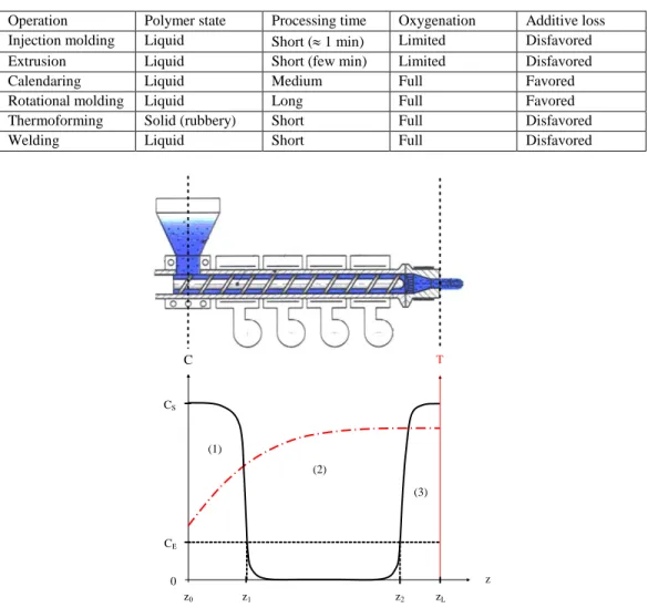
In the case of injection or extrusion molding, the molten polymer is partially confined within the pressurized zone of the reactor. Indeed, oxygenation is limited to air/molten polymer interfaces at the feeder and die. Oxygen concentration is thus highest at both extremities and decreases rapidly towards the center of the reactor because oxidation is

oxygen diffusion controlled (Audouin et al. 1994). Moreover, the temperature is not homogeneous in the reactor. Thus, thermal oxidation occurs in a non-isothermal regime.

The resulting profiles of oxygen concentration and temperature have been schematized in Figure 7.

According to this simplified scheme, two different zones can be distinguished in an injection or extrusion machine:

 “Well-oxygenated” zones (1 and 3) in which regime E (high oxygen concentration) leads to a predominant chain scission process,

Table 5. Characteristics of usual processing operations of thermoplastics

Operation Polymer state Processing time Oxygenation Additive loss Injection molding Liquid Short ( 1 min) Limited Disfavored Extrusion Liquid Short (few min) Limited Disfavored Calendaring Liquid Medium Full Favored Rotational molding Liquid Long Full Favored Thermoforming Solid (rubbery) Short Full Disfavored Welding Liquid Short Full Disfavored

z0 z CE CS z1 z2 zL 0 (1) (2) (3) C T

Figure 7. Schematization of the profiles of oxygen concentration C and temperature T in an injection or extrusion reactor. Coordinates zL and z0 are the location of the air/molten polymer interfaces at the

feeder and die respectively. Coordinates z1 and z2 are the limits between the “well-oxygenated” zones

 And “poorly oxygenated” zone (2) in which regime L (low oxygen concentration) leads to predominant chain extension and branching processes, and eventually crosslinking.

Thus, it appears that the relative predominance of both types of macromolecular changes depends on four factors:

 The screw length: L = zL – z0.

 The length of both “well-oxygenated” zones: 1 = z1 – z0 and 3 = zL – z2.  And the residence time te.

Lengths 1 and 3 depend, in turn, on five parameters:

 The equilibrium oxygen concentration CS and the rate of oxygen consumption r(CS)

at the air/molten polymer interfaces.

 The oxygen diffusivity DO2 into the molten polymer.  The temperature profile in the reactor.

 And the rate of polymer transport along the screw.

As seen in Eq. 18, CS is temperature independent. However, the ratio DO2 /r(CS) is a

decreasing function of temperature (Audouin et al. 1994). It is thus expected that: 1 > 3. It is thus possible to define two extreme types of injection or extrusion machines:

a) “Well-oxygenated” reactors, characterized by large feeder and die sections and short screw (1 > 3 >> 2), favoring chain scissions.

b) And “poorly oxygenated” reactors, characterized by narrow feeder and die sections, and long screw (2 > 1 > 3), favoring chain extensions and branchings.

PET mechanical recycling by extrusion has been recently reviewed by Nait-Ali et al. (2011). In the majority of cases (La Mantia and Vinci 1994, Paci and La Mantia 1998, Frounchi 1999, Spinacé and De Paoli 2001, Oromiehie and Mamizadeh 2004, Badia et al. 2009, Romao et al. 2009), melt re-processing leads to a large predominance of chain scissions, which results in the monotonous decreases in the weight average molar mass MW

and melt viscosity . However, in two cases (Assadi et al. 2004, Nait-Ali et al. 2012), chain extensions and branchings are also observed and can, finally, predominate over chain scissions. After a certain time of exposure, depending on the aggressiveness of the thermal exposure conditions, they lead to a re-increase in MW and . In one case (Assadi et al. 2004),

polymer gelation (by crosslinking) is even observed during the fourth extrusion cycle, causing a complete obstruction of the extruder. In this latter, the almost total confinement of the molten polymer within the pressurized zone of the reactor favors clearly the regime L.

Calendaring and, especially, rotational molding are characterized by a long exposure time of the molten polymer at high temperature in air. In the case of rotational molding, this duration takes several dozens of minutes, which constitutes extreme thermal ageing conditions for polymers. Antioxidant loss by evaporation and chemical consumption are strongly favored at the air/molten polymer interface. As an example, the formation of a

superficial oxidized layer of about 300 µm thick has been evidenced in the case of iPP (Sarrabi et al. 2010). That is the reason why this process is usually considered as the most critical from the point of view of polymer degradation.

Thermoforming is expected to be “less degrading” owing to the lower maximum temperature. In contrast, degradation at a noticeable extent can be observed in certain cases of welding (by hot air streams), where the shortness of the hot stage cannot compensate the (sometimes very high) maximum temperature of exposure.

3. P

P

3.1. Temperature



Molar Mass Maps

A given processing operation is characterized by an optimal viscosity range corresponding to values of melt flow index (MFI) typically ranged between less than 0.1 (for pipe extrusion) and more than 10 (for paper coating). Schematically, the MFI is proportional to the reciprocal of the melt viscosity, this latter being an increasing function of the polymer molar mass. In the domain of low shear rate where the viscosity can be approximated by its Newtonian value, one can write:

4 . 3 W

KM

MFI



where K is an increasing function of temperature.

It appears thus convenient to study the processability conditions in a temperaturemolar mass map. Three important boundaries can be defined in such a map:

a) The solidrubbery/liquid boundary, i.e. the glass transition temperature (Tg) for

amorphous polymers or the melting temperature (Tm) for semi-crystalline polymers.

Both temperatures are increasing functions of molar mass in the domain of low molar mass where M < MC, MC being the entanglement threshold (Fetters et al. 1999). Tg

continues to increase with Mn above MC according to the FoxFlory law (1954):

n FF g g

M

K

T

T





where KFF is the order of 10100 K.kg.mol -1

, so that Tg tends to be almost independent of

molar mass when this latter is higher than 10100 kg.mol-1. KFF is an increasing function of

Tg (which depends essentially on the chain stiffness).

Tm tends to decrease very slowly with the chain length far above MC because the

entanglements tend to perturb crystallization.

b) The rubber/liquid boundary TL, which can be more or less arbitrarily defined as the

of the complex shear modulus), the terminal relaxation time (Mark et al. 2004), etc. For a shake of simplicity, this boundary can be defined as follows: For a given shear rate , the melt viscosity can be expressed as the product of two functions:

)

M

(

g

)

T

(

f





Let us consider the high viscosity limit for the processing operation under consideration:

)

M

(

g

)

T

(

f





)

M

(

g

)

T

(

f





T

f

g

(

M

)

F

(

M

)



















Thus, for a given molar mass M, this function represents the boundary: TL = F(M) such

as:

- For T < TL, the polymer would have a melt viscosity too high to be processable,

- Whereas, for T > TL, it would be, in principle, processable.

In the case where the Newtonian viscosity obeys an Arrhenius law, one would have (for MW > MC): 4 . 3 W V 0 max

M

RT

H

exp

K

_























that leads finally to:

4 . 3 W 0 m ax V L

M

K

Ln

R

H

T





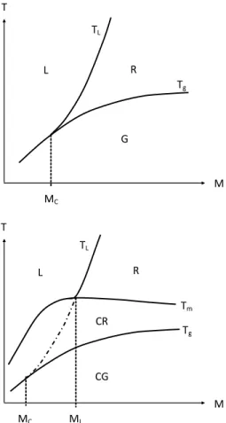
T M ML CG R L Tg TL Tm CR MC T M MC G R L Tg TL

Figure 8. Shape of the temperaturemolar mass map (in a logarithm scale for M) for an amorphous polymer (top) and a semi-crystalline polymer (bottom).

Legend: G: glassy domain; R: rubbery domain; L: liquid domain; CG: semi-crystalline polymer with amorphous phase in glassy state; CR: semi-crystalline polymer with amorphous phase in rubbery state.

In all cases, there is a critical molar mass MC corresponding to the onset of the

entanglement regime. Schematically, for an amorphous polymer:

TL Tg at M  MC (32)

TL > Tg at M  MC (33)

In this later case, (TL – Tg) is an increasing function of M.

In a same way, for a semi-crystalline polymer, there is a molar value ML higher than MC

such as:

TL Tm at M  ML (34)

ML can be defined as the molar mass for which the length of the rubbery plateau

corresponds to the distance between Tm and Tg.

Most of the processing operations for thermoplastics (except thermoforming or machining) involve, at least, one elementary step in liquid state, i.e. above TL. But, thermal

degradation limits the accessible temperature range.

3.2. Thermal Stability Ceiling

The temperature at the degradation threshold can be defined from the quantities and relationships established in section 1.2. If xD is the endlife criterion for the conversion ratio of

the degradation process, it is possible to define an “equivalent isothermal temperature” TD

such as: when Te = TD, xe = xD. In other words, degradation would just reach the endlife

criterion at the end of the processing operation if Te = TD. In this case:

0 D W

r

x

)

t

(

F



So that, according to Eq. 10:















t

r

x

Ln

R

H

T

3.3. Brittle Limit

All the polymers are brittle when their molar mass is lower than a critical value MF.

Amorphous polymers (PC, PMMA, PS, etc.) and highly or moderately polar semi-crystalline polymers, having their amorphous phase in glassy state (PA 6, PA 6-6, PA 11, PET, etc.), are characterized by a MF value close to the entanglement threshold (Kausch et al. 2001):





F

5

10

M

M





Ductility and toughness are thus essentially linked to the existence of an entanglement network.

In contrast, apolar semi-crystalline polymers, having their amorphous phase in rubbery state (PE, PP, POM, PTFE, etc.), are characterized by a considerably higher ductilebrittle transition (Fayolle et al. 2008):





F

50

60

M

M





This peculiarity seems to be linked to the fact that molar mass changes are not directly responsible for embrittlement. Indeed, in this last case, the causal chain would be rather:

Polymer oxidation → PO° radicals → Chain scissions → Chemicrystallization → Decrease in interlamellar spacing la → Embrittlement

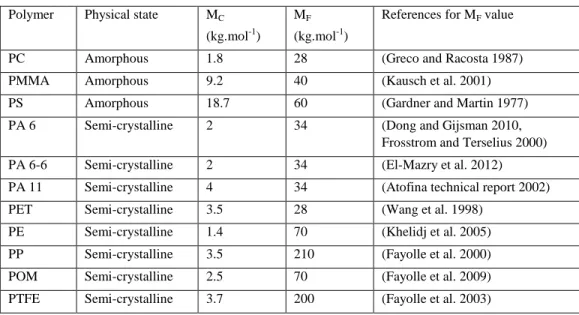
Table 6. Entanglement threshold and ductilebrittle transition of some usual amorphous and semi-crystalline polymers

Polymer Physical state MC

(kg.mol-1) MF

(kg.mol-1)

References for MF value

PC Amorphous 1.8 28 (Greco and Racosta 1987) PMMA Amorphous 9.2 40 (Kausch et al. 2001) PS Amorphous 18.7 60 (Gardner and Martin 1977) PA 6 Semi-crystalline 2 34 (Dong and Gijsman 2010,

Frosstrom and Terselius 2000) PA 6-6 Semi-crystalline 2 34 (El-Mazry et al. 2012) PA 11 Semi-crystalline 4 34 (Atofina technical report 2002) PET Semi-crystalline 3.5 28 (Wang et al. 1998)

PE Semi-crystalline 1.4 70 (Khelidj et al. 2005) PP Semi-crystalline 3.5 210 (Fayolle et al. 2000) POM Semi-crystalline 2.5 70 (Fayolle et al. 2009) PTFE Semi-crystalline 3.7 200 (Fayolle et al. 2003)

As an example, the critical value of la is about 67 nm for PE (Kennedy et al. 1994).

Indeed, using extreme crystallization conditions, these authors have shown that it is possible to obtain such a critical value laF even for PE having a molar mass significantly higher than

100 kg.mol-1.

However, in the practical case of common processing conditions, laF corresponds to a MF

value of (70  30) kg.mol-1.

MF constitutes an important vertical boundary in the temperaturemolar mass map:

Polymers are easily processable below MF, but they cannot be used, in practice, owing to their

very high brittleness. MF is of the order of 2030 kg.mol -1

for many usual amorphous polymers and polar semi-crystalline polymers. In contrast, MF is of the order of 100200

kg.mol-1 for apolar semi-crystalline polymers. Examples of values have been reported in Table 6.

3.4. Processability Window

It is then possible to build the temperaturemolar mass map for a given amorphous polymer. It must have, in the most common cases, the shape of Figure 9.

Let us consider the intersection point D between the thermal stability ceiling TD and the

“rheological threshold” TL. It corresponds to a molar mass MD which can be defined as

follows: For M > MD, processing (for the temperaturetime history under consideration) is

impossible because the material cannot be maintained in its liquid state for the desired duration without undergoing a catastrophic thermal degradation. Thus, each polymer is

characterized by a molar mass interval [MF, MD in which it is possible to process parts with

acceptable mechanical properties.

D T M MC Tg TL TD MF MD

Figure 9. Shape of the temperaturemolar mass map for an amorphous polymer. The dashed zone corresponds to the processability window.

3.5. Usual Ways to Widen Processability Window

The processability window appears as a trigonal domain for which the ductilebrittle transition MF is a material property which cannot be, in principle, shifted. There are thus only

two ways to widen the processability window, corresponding to the shifts of the two remaining boundaries (Figure 10).

Let us notice that there are cases where the thermal stability ceiling of the unstabilized polymer is so low as MD < MF. In this case, there is no way to process this polymer in the

entangled regime (Figure 12). PVC and PP, for instance, belong to this polymer family: There is no way to process these polymers without an efficient system of stabilization, which explains the large amount of literature works devoted to their thermal stabilization.

PVC is a very interesting, but complicated, case because some of its stabilizers, e.g. metal soaps, can act as lubricants whereas others, e.g. alkyltin thioglycolates, display a significant plasticizing effect. A complete understanding of these stabilization mechanisms needs, no doubt, the detailed knowledge of both chemical and physical aspects.

An interesting peculiarity of PP is its very high critical molar mass MF 210 kg.mol -1

. Thus, embrittlement can occur at an extremely low conversion of the oxidation process, practically undetectable by chemical or spectrochemical titrations (Fayolle et al. 2004). Such a characteristic explains well the relative sensitivity of this polymer to recycling by melt re-processing.

Let us notice that, in the (very frequent) case where the polymer perishes by oxidation, it is possible to envisage a significant widening of the processability window by inerting the air/molten polymer interfaces (see Figure 7 for injection and extrusion molding), especially by nitrogen. This effect could be schematized by Figure 10 (bottom) or Figure 11, TD and T’D

T M Tg TL TD T’D T M Tg TL TD T’L T’g

Figure 10. Shift of the boundaries of the processing window by modifications of an amorphous polymer composition. Top: Use of processing aids (plasticizers, oils, lubricants, etc.). Bottom: Use of thermal stabilizers. The dashed line corresponds to the starting polymer boundaries and the arrows indicate the effects of these modifications.

T M MC Tg TL T’D MF MD TD

Figure 11. Shape of the temperaturemolar mass map for a non-processable amorphous polymer: In the absence of stabilizers (TD), MD < MF, there is no way to process a ductile/tough polymer. Thanks to an

efficient system of stabilization (T’D), MD is shifted beyond MF and a processability window appears

(dashed area). The dashed line corresponds to the starting polymer boundaries and the arrow indicates the effect of this modification.

4. C

P

P

4.1. PET Characteristics

PET is a semi-crystalline polymer with a melting point Tm ranged between 240 and

250°C. The processing temperature cannot be lower than Tm. It is usually chosen between 250

and 280°C (Nait-Ali et al. 2011). The ductilebrittle transition MF of PET is about 28 kg.mol

-1

(Wang et al. 1998). For industrial grades, the weight average molar mass MW0 is ranged

between 55 and 65 kg.mol-1, and the polydispersity index p0 is close to 2 (Nait-Ali et al.

2011). Since MW0  70 kg.mol -1

, the number of chain scissions nF to reach embrittlement is

thus very low. According to Eq. 11:

70

2

M

2

n





This value must be compared to the monomer unit concentration:





CRU

m

1

CRU



where mUCR is the molar mass of the (repetitive) monomer unit: mCRU = 192 g.mol -1

.

i.e. [CRU] = 5.2 mol.kg-1

PET displays three very important characteristics at 250280°C: - The existence of ester groups extremely reactive with water.

- The existence of structural irregularities, i.e. diethylene glycol units, highly unstable at these temperatures. Although their represent only between 1 and 3.6 mol% of the total monomer units (MacDonald 2002), their thermal decomposition can significantly affect the PET rheological behavior in the absence of oxygen.

- And the existence of ethylene oxide sequences highly reactive with oxygen (see Table 2).

Thus, three main chemical processes are expected to occur in the temperature range of an injection or extrusion processing operation:

 Hydrolysis/condensation,

 Anaerobic thermal decomposition,

4.2. Hydrolysis/Condensation

The mechanistic scheme can be written:

Es + W Al + Ac

where Es designates an ester group, W the water molecule, and Al and Ac the carboxylic acid and alcohol chain ends respectively. These latter are assumed to be initially (before processing) in equal concentrations: [Al]0 = [Ac]0 = [A]0.

kH and kC are the rate constants of hydrolysis and condensation reactions respectively.

Hydrolysis is expected to predominate if the initial water concentration is higher than the equilibrium concentration: 0 2 0 H C

]

Es

[

]

A

[

k

k

]

W

[



The number of chain scissions at equilibrium is thus:

0 2 0 H C 0 0

]

Es

[

]

A

[

k

k

]

W

[

]

W

[

]

W

[

n









In fact, in polyesters, the ratio kC /kH is relatively low and [A]0 2 /[Es]0 10 -4 , so that: 0

]

W

[

n



The number of chain scissions is thus almost equal to the initial number of water molecules. As a result, [W]0 must be significantly lower than 4.3  10

-2

mol.kg-1, i.e. 770 ppm, to avoid embrittlement (see Eq. 40).

As an indication, this value (770 ppm) is about 15 times lower than the equilibrium water concentration in PET at ambient temperature.

All these characteristics are well known by practitioners. It is generally considered that hydrolysis can induce a catastrophic decrease of the melt viscosity during processing if the water concentration exceeds a critical value of about 100200 ppm (Zimmermann 1984, Scheirs 1998).

That is the reason why, to avoid totally hydrolysis, PET granules/flakes are carefully dried prior to processing. On the other hand, heating in dry state (i.e. when [W]0 < [W])

favors condensation and thus, allows to restore high molar mass values in hydrolytically degraded samples (Lamba et al. 1986).

The effects of the hydrolysis/condensation process on the polymer structure can be thus considered as reversible at long term, because it offers always the possibility to “repair” chain scissions.

kH

→ ← kC

4.3. Anaerobic Thermal Degradation

Esterification and transesterification reactions are expected to occur at high temperature in PET (Goodings 1961, Buxbaum 1968, Zimmermann 1984, Culbert and Christel 2003). It can modify the molar mass distribution until an equilibrium distribution is reached. It can also generate macrocycles as observed by MALDI TOF experiments (Ma et al. 2003). But, in the absence of oxygen, PET degrades essentially by a non-radical mechanism involving a rearrangement of the ester groups of ethylene glycol units (i.e. monomer units):

C O O CH2 CH H C OH O + H₂C CH

This mechanism can be rewritten:

(0) Es → POH=O + FV (k0)

where POH=O and FV designate carboxylic acid and vinylidene chain ends respectively.

This mechanism has been investigated by many authors (Pohl 1951, Marshall and Todd 1953, Goodings 1961, Buxbaum 1968, Zimmermann 1984, McNeil and Bounekhel 1991, Montaudo et al. 1993, Khemani 2000, Samperi et al. 2004, etc.). It can be considered, in a first approach, as irreversible. It is very slow in usual processing conditions and predominates only at long term when the hydrolysis/condensation process has reached its equilibrium (Assadi et al. 2004). The resulting changes in melt viscosity have been schematized in Figure 12.  t (2) (1) (1) + (2)

Figure 12. Shape of the changes in melt viscosity during an isothermal exposure at 280°C in dry nitrogen. The curve displays a maximum linked to the existence of two distinct contributions (dashed lines): Condensation (1) and anaerobic thermal degradation (2).

Let us return to the effects of the hydrolysis-condensation process. The equilibrium molar mass is:

 





_

A

b

2

M

2

M

where [A] is the equilibrium concentration of carboxylic acid (or alcohol) chain ends such

as:

 

   

_Es

_W

k

k

A

_













and b is the half concentration of non-condensable chain ends, e.g. vinylidene double bonds. The above described thermal degradation process would thus lead to an increase of b according to a zero-order kinetics:

t

r

b

b





where rS is the corresponding rate of chain scissions for this mechanism.

In the case of a single processing operation, this process is expected to have non-significant consequences. But, the corresponding structural defects accumulate irreversibly after several melt re-processing operations, contrarily to those induced by hydrolysis. Thus, after N mechanical recycling operations, one could reach a value of b higher than the critical number of chain scissions necessary to reach the structural embrittlement criterion nF. In other

words, the molar mass would be lower than MF, even in dry equilibrium state, and the

polymer would be permanently brittle.

PET chains can also contain weak structures, for instance diethylene glycol units which are considered as the main structural irregularities (MacDonald 2002). Ester groups belonging to these structures degrade more easily than normal esters. They can be responsible for a fast, but limited, degradation step obeying to a first-order kinetics (Nait-Ali et al. 2011):

Kt

exp

'

b

'

b





where K is the pseudo first-order rate constant for this mechanism.

4.4. Thermal Oxidation

According to well established structure-property relationships, oxidation is expected to attack preferentially methylene groups in PET (Korcek et al. 1972). Thus, the mechanistic scheme of thermal oxidation of molten PET can be derived from the “closed loop” mechanism established for common poly(methylenic) substrates at low temperature (typically for T < 200°C), in particular for PE (see section 2.1). However, at higher temperature (typically for T  250°C), this mechanistic scheme must be slightly improved and complete:

a) The hydroperoxide critical concentration [POOH]C, beyond which thermal

mode (Ib), is an increasing function of temperature (Colin et al. 2004). It is about 9.2

 10-1 mol.l-1 at 250°C (Khelidj et al. 2006). It is thus necessary to accumulate a considerable quantity of POOH groups to initiate the bimolecular mode. Thus, above 250°C, one can reasonably consider that POOH decomposition is essentially unimolecular.

b) Molecular oxygen is a bi-radical in ground state. Thus, it cannot be excluded that it reacts directly with the polymer for abstracting labile hydrogens. In a first approach, this reaction can be written (Nait-Ali et al. 2011):

(Io) PH + O2 → 4P° + 2H2O (k1o)

c) At 30°C, the reactivity of methylenes in PET is about six times higher than in PE, because of the presence of an oxygen heteroatom in  position (see Table 2). However, this difference in reactivity reduces as the temperature increases. Above 250°C, it becomes negligible.

d) Above 250°C, peroxides POOP cannot survive. Thus, disproportionation is the only way of termination of PO2° radical pairs. It leads to the formation of alcohol and

anhydride groups: C O O CH CH2 O 2 + C O O C CH2 O C O O CH CH2 OH O O2 +

e) Aldehydes are the main carboxylic chain ends formed by chain scissions. They result from the  scission of alkoxy radicals PO°. However, their hydrogen is considerably more labile (ED ≈ 368 kJ.mol

-1

) than those of methylene oxide groups (ED ≈ 376

kJ.mol-1). That is the reason why, as soon as they are formed, aldehydes oxidize quasi-instantaneously into carboxylic acids (Nait-Ali et al. 2011):

C O O CH CH2 O C O O C O O C CH2 O C O O H + CO2 C CH2 O C O O HO +  scission

 scission several oxidation steps

f) As seen in the previous section, non-radical mechanisms can also take place above 250°C and thus, superimpose to radical chain oxidation. Among these potential

mechanisms, two are the subject of a relative consensus in the literature and, for this reason, must be taken into account:

 The rearrangement of the ester groups of structural irregularities (see section 4.3):

(0i) Irreg → POH=O + FV (k0i)

 The condensation of pairs of carboxylic acid chain ends (Khemani 2000, MacDonald 2002, Lecomte and Ligat 2006, Ciolacu et al. 2006, Romao et al. 2009) leading to the formation of anhydride groups:

C CH2 C O O C CH2 O C O O OH 2 C O O CH2 C O O O H2O +

This mechanism can be rewritten:

(VII) POH=O + POH=O → O(P=O)2 + H2O (k7)

where O(P=O)2 designates anhydride groups.

From a careful FTIR real-time analysis of molten PET at 280°C under two different oxygen partial pressures (1% and 21% of atmospheric pressure), Nait-Ali et al. (2011) observed the appearance and growth of several overlapped bands in the 17601820 cm-1 region, which can be effectively attributed to the formation anhydride groups.

A very important characteristic of thermal oxidation of molten PET is that it leads to a predominant chain scission process at high oxygen concentration and a predominant chain extension and branching (and eventually crosslinking) processes at low oxygen concentration. Both regimes necessarily coexist in the case of injection or extrusion molding as the result of the oxygen concentration gradients schematized in Figure 7. Their existence has been demonstrated from rheometric experiments.

Indeed, the rheometer cavity is an ideal reactor for studying the PET macromolecular changes induced by thermal oxidation in carefully controlled (temperature, oxygenation and shearing) conditions:

 The temperature field is homogeneous and perfectly regulated.

 The atmosphere can be perfectly controlled and rapidly changed.

 The shear amplitudes are sufficiently low to ensure the absence of mechano-chemical degradation.

 The equipment gives a direct information on the weight average molar mass MW with

a high sensitivity.

1) Under a constant oxygen partial pressure: 0%, 0.6%, 1%, 9% and 21% of atmospheric pressure, in order to reproduce the local macromolecular changes (i.e. the relative predominance of chain scissions or chain extensions/branchings) at a given oxygen concentration, i.e. at a given z position in the extruder reactor. The corresponding changes in Newtonian viscosity  are presented in Figure 13. These results call for the following comments:

Figure 13. Changes in Newtonian viscosity of PET at 280°C under various oxygen partial pressure: 0% (0); 0.6% (1); 1% (2); 9% (3) and 21% of atmospheric pressure (4).

 As expected, in the absence of oxygen (0% of atmospheric pressure), PET is relatively stable. After a very slight decrease, which can be reasonably attributed to the thermal decomposition of main structural irregularities (i.e. diethylene glycol units),  reaches an asymptotic value.

 At low oxygen partial pressures (typically for pO2 < 9% of atmospheric pressure), 

increases slowly until the complete polymer gelation. Thus, chain extensions/branchings prevail on chain scissions. At higher oxygen partial pressures, however,  decreases sharply with the time of exposure. Chain scissions predominate largely over chain extensions/branchings.

 The critical oxygen partial pressure pE delimiting the “well-oxygenated” zones from

the “poorly oxygenated” zone in the extruder reactor is about 9% of atmospheric pressure, i.e. 9  103 Pa. The numerical application of Eq. 18 leads to:

CE = 4.2  10 -4

mol.l-1 for PET at 280°C (Nait-Ali et al. 2011).

2) Under a variable oxygen partial pressure, ranged between 0% and 21% of atmospheric pressure, in order to reproduce the historical background of macromolecular changes (sequences of chain scissions and chain extensions/branchings) during a complete extrusion operation. The polymer was exposed under nitrogen, but with short admissions of air under atmospheric pressure (during approximately 2 minutes). The corresponding changes in Newtonian viscosity  are presented in Figure 14. These results call for the following comments:

0.4 0.6 0.8 1.0 1.2 1.4 1.6 0 25 50 75 100 125 150 175 200  (t ) /  (t = 0) time (min) (2) (1) (3) (4) (0)

- The first stage corresponds to a phase of “stabilization” in nitrogen. After a very slight decrease, which can be reasonably attributed to the thermal decomposition of the main PET structural irregularities (i.e. diethylene glycol units),  reaches an asymptotic value.

- The second stage corresponds to a dramatic drop of  in air. In this narrow interval, nitrogen has been replaced by air under atmospheric pressure during approximately 2 minutes. Thus, chain scissions predominate largely over chain extensions/branchings. One can notice the absence of induction time, since the decreasing rate of  is maximum from the introduction of air into the rheometer cavity. This is an important argument in favor of the existence of an extrinsic initiation of thermal oxidation: The direct reaction of molecular oxygen with the polymer (Io) allows to describe, without the use of an additional assumption or adjustable parameter, this important characteristic of the thermal oxidation kinetics of molten PET at 280°C.

- The third stage corresponds to a non-monotonous change in  when the oxygen partial pressure decreases from 21% to 0% of atmospheric pressure. In this interval, air has been replaced by nitrogen, until the complete stabilization of . One observes, at first, a slowdown of the  decrease, previously initiated in air, leading to a minimum value of , presumably reached when the oxygen partial pressure equals 9% of atmospheric pressure. It is, indeed, at this critical value that chain extensions/branchings equilibrate chain scissions (see Figure 13). Once the oxygen partial pressure becomes lower than this critical value, chain extensions/branchings predominate over chain scissions and  re-increases. This final increase stops when oxygen is totally consumed in the rheometer cavity.

250 300 350 400 450 500 0 20 40 60 80 100 120 140  (Pa.s) time (min) Nitrogen Nitrogen Nitrogen Air Air

Figure 14. Changes in Newtonian viscosity of PET at 280°C during two nitrogen/air alternations under atmospheric pressure. Duration of successive exposures under nitrogen: 42 min, 53 min then 40 min. Duration of exposures under air: 2 min in both cases.