Science Arts & Métiers (SAM)
is an open access repository that collects the work of Arts et Métiers Institute of Technology researchers and makes it freely available over the web where possible.
This is an author-deposited version published in: https://sam.ensam.eu Handle ID: .http://hdl.handle.net/10985/6755
To cite this version :
Annie-Claude BAYEUL-LAINE, Sophie SIMONET, Gérard BOIS, Abir ISSA - Two-phase numerical study of the flow field formed in water pump sump: influence of air entrainment - IOP Conference Series: Earth and Environmental Science p.1-12 - 2012
Any correspondence concerning this service should be sent to the repository Administrator : archiveouverte@ensam.eu
Two-phase numerical study of the flow field formed in water
pump sump: influence of air entrainment
A C Bayeul-Lainé1, S Simonet1, G Bois1, A Issa2
1Arts et Metiers PARISTECH, LML, UMR CNRS 8107, 8, Boulevard Louis XIV 59046 LILLE Cedex, France
2Faculté de Génie Civil, Université de Damas, Baramkeh-Mazzé, Syrie E-mail: Annie-claude.bayeul-laine@ensam.eu
Abstract. In a pump sump it is imperative that the amount of non-homogenous flow and entrained air be kept to a minimum.Free air-core vortex occurring at a water-intake pipe is an important problem encountered in hydraulic engineering. These vortices reduce pump performances, may have large effects on the operating conditions and lead to increase plant operating costs. The purpose of this paper is to reproduce the flow pattern of experiments and to confirm the geometrical parameter that influences the flow structure in such a pump. The numerical model solves the Reynolds averaged Navier-Stokes (RANS) equations and VOF multiphase model. STAR CCM+ with an adapted mesh configuration using hexahedral mesh with prism layer near walls was used. Attempts have been made to calculate two phase unsteady flow for stronger mass flow rates and stronger submergence with low water level in order to be able to capture air entrainment. The results allow the knowledge of some limits of numerical models, of mass flow rates and of submergences for air entrainment. In the validation of this numerical model, emphasis was placed on the prediction of the number, location, size and strength of the various types of vortices coming from the free surface.
1. Introduction
This work is an extended study starting from 2006 (Bayeul-Lainé and al. [1], Issa [2] in LML and first published by Issa and al. in 2008 and 2009 [3-4]. Several cases of sump configuration have been numerically investigated using one specific commercial code and are based on the initial geometry proposed by Constantineascu and Patel [5]. The results, obtained with a structured mesh, were strongly dependent on main geometrical sump configuration such as the suction pipe position, the submergence of the suction pipe on one hand and the turbulence model on the other hand. Part of the results shows a good agreement with experimental investigations already published by the Iowa Institute of Hydraulic Research [6-10] to reduce non uniformities of specific flow and geometrical conditions. More basic studies have been also conducted to establish empirical criteria for vortex formation and avoidance [11-13]. More recently, CFD Benchmarks have been performed by Matsui and al. [14] in order to compare different software results with experiments. Numerical simulations were realized by Isabasoiu and al [15] with the commercial code FLUENT 6.0. These simulations didn’t take account air entrainment. The goal of the numerical approach used in this paper was to find the influence of the level upstream in the intake channel to the suction sump in the swirling flow development. Few papers were found discussing about air entrainment. The main difficulty was to take account the effect of free surface and to model it.
Lucino and al [16] verified the ability of commercial CFD (computational fluid dynamics) code to predict the formation of vortices in a pump sump with FLOW 3D using the LES (Large Eddy Simulation). The free surface was tracked by means of a split lagrangian method for the advection of the VOF (volume of fluid). The fluid was considered monophasic and incompressible. The numerical results demonstrated the capability of the model identifying the observed vortices in the physical model. The calculated vorticities with the highest values were consistent with the air-entrained vortices. The floor vortex reached the highest vorticity magnitude and suggested the possibility of a cavitating core at the operating condition of lower submergence.
Shulka and al [17] used the commercial code CFX to carry out two-phase flow simulation to capture air entrainment. They used a steady state solution. Turbulence was modelled by a k- model. The paper dealt with numerical and experimental results. The CFD model predicted the flow in sufficient details to identify the locations, size and the strength of the vortices. The air entrainments and its location were well captured. The results were in accordance with the experimental investigation.
2. Experimental geometrical models
The experimentations were realized by Issa Abir in the Hydraulic Laboratory at “Université de Génie Civil” in Damas.
The main aim of this experimental study was to detect the best position of the intake pipe which didn’t lead to troubles at the inlet of the pump. It is essential to ensure that a pump intake supply water with the most uniform velocity at the entry of the impeller. The fluid flow in pump intakes is rather complex, often with swirl-free flows.
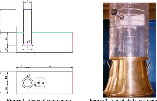
The experimental apparatus consisted of a closed loop containing a sump (Figure 1), the water-sump pump realized in transparent acrylic walls, a centrifugal pump, a metallic pipe at the outlet of the pump, a flow rate-meter (Figure 2), a valve to control the mass flow rate. The following measures were realized: the tangential velocity in the pipe, the static pressure at the wall of the inlet pipe for different angles, the pressure on different parts of the loop, the mass flow rate. Formations of free surface vortices and subsurface vortices were visually observed.
Figure 1. Shape of sump pump Figure 2. four-bladed swirl meter
192 cases were tested by combining parameters given in table 1. These parameters are given in function of baffle intake interior diameter D (D=180 mm). These parameters are the depth of the sump b, the distance l between the pipe and the back side of the sump, the clearance distance from floor z and, the submergence depth for the pipe h. All measures were realized for a constant flow rate of Qm equal to 18 kg/s and for the following non dimension numbers: Red = 1,8 105; 5.56 104 < Reh < 8.33
104; Fr = 1.45; We = 6160.
Table 1 Parameters for experimentation b/D l/D z/D
1.5 0.5 0.3
2 0.75 0.5
2.5 1 0.75
3 1.25 1
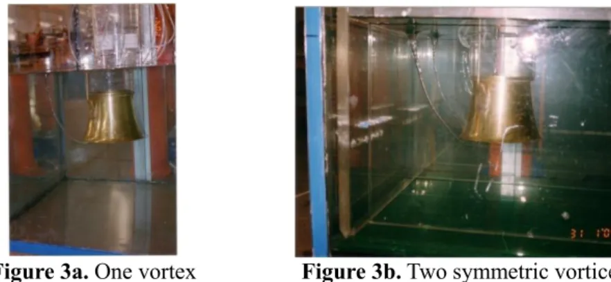
The experimental investigation revealed that there is formation of air entrainment when b and h are small. All air entrainment vortices locate along the height between the pipe and the back wall. One or two air entrainment vortices have been observed. For example, two symmetric swirls can be observed in Figure 3b for l=1,25D. If b is small, sometimes, only one air entrainment vortex appears, as can be observed in Figure 3a. This swirl is often located in the middle of the sump.
Figure 3a. One vortex Figure 3b. Two symmetric vortices
It has been found that the most important parameters that influence the occurrence of air entrainment are the depth of the sump b, the distance between the pipe and the back wall l, the submergence depth of the pipe h and the clearance distance from floor z.
Increasing the value of l increases the potential air entrainment vortices. The size and the magnitude of these swirls increase too.
When b increases, the air entrainment vortices decrease in magnitude until they become vortices with no air entrainment or decrease to finally disappear.
The beginning and the magnitude of these swirls decrease with the increase of the values of z. When z is equal to the diameter of the bell mouth D, the air entrainment swirl have a low magnitude if b is high (b/D>2.5) and l small. This is the case for low velocity at the free surface.
Increasing the value of h decreases the possibility of air entrainment vortices
3. Numerical models
The simulations were performed with the commercial code Star CCM+ V6.06. 3.1. Physics, boundary and initial conditions
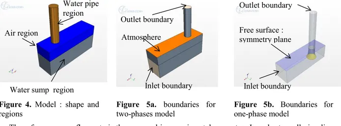
The main difficulty of such simulations is to well represent the behaviour of the free surface. In previous studies [1-4], one phase models were tested with a symmetry plane boundary at the free surface. In order to have a reference model, calculations with one phase model were also realized here too. The same calculations were done with two phases model (water and air phases) in case of steady state and in case of unsteady state (Figures 4, 5a and 5b).
In order to well represent air entrainment, according to experimental results, the next parameters were chosen as a reference numerical case: b/D=1.5; l/D=1.25; h/D=1.2; z/D=0.3. Experimentations pointed out air entrainment in this specific case. Tests with a lower submergence depth of the pipe h equal to D were also realized.
Figure 4. Model : shape and
regions
Figure 5a. boundaries for two-phases model
Figure 5b. Boundaries for one-phase model
The reference mass flow rate is the one used in experimental apparatus. In order to well visualize the air vortices, numerical tests with higher mass flow rate were also calculated.
The calculation domain was divided into three zones: the air zone, the sump zone and the pipe zone. So for the simulation of the sump pump three linked meshes were used as it can be seen in Figures 4, 5a and 5b.
The boundary condition at the inlet consisted of a mass flow rate (18 and 24 kg/s).
The boundary condition at the outlet was the same constant mass flow rate going out of the domain. This was located at the top face of the pipe.
The boundary condition at the free surface used for the single phase model is symmetry. For the two phases model, the horizontal boundary of the air region is an absolute pressure inlet equal to atmospheric pressure.
For the single phase model, the fluid (water) was considered incompressible. For the two phases model, the fluid was considered biphasic (air and water), incompressible for the water phase and as an ideal gas for the air phase, at a constant temperature of 20ºC.
Buoyant option, with density difference fluid buoyant model, is assigned to all domains. Buoyant reference density of air is assigned to all domains. The gravity acceleration was set to 9.81 m/s².
Two turbulence models were tested: the realizable two-layer k- model which combines the Realizable k-model [18] with the two-layer approach [19] and the SST k- model [20].
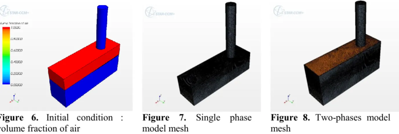
Volume of Fluid (VOF) is used to model the interaction between the two phases. It is a simple multiphase model that is well suited to simulate flows of several fluids on numerical grids capable to resolve the interface between the mixture’s phases. The two phases are assumed to share the same velocity, pressure and temperature fields. As a consequence, the same set of basic governing equations describing momentum, mass and energy transport in a single-phase flow is solved for an equivalent fluid whose physical properties are calculated as functions of the physical properties of its constituent phases and their volume fractions. The initial condition for the volume fraction of phase is given in figure 6: air for air region (in red) and water for water pipe region and water sump region (in blue).
A steady state solution can depict the formation of an air core but it is well known that the phenomena are always transient. Previous numerical studies were realized with steady one phase model, so steady one phase models were modeled here in order to make comparisons. Then steady and unsteady two phases models were calculated in different cases. The steady models are used as initial conditions for the unsteady models.
3.2. Grids and simulations
A multi-domain model allows using different target sizes. Mesh was refined in pipe zone and in the interface between air and water at free surface. A polyhedral mesh with prism layers is used for all calculations (7 prism layers in the sump and 10 in the pipe). A growth rate of 1.02 is used (Figures 7 and 8). All test cases are resumed in table 2.
Air region
Water pipe region
Water sump region
Atmosphere Outlet boundary
Inlet boundary Inlet boundary Outlet boundary Free surface : symmetry plane
Figure 6. Initial condition :
volume fraction of air
Figure 7. Single phase
model mesh
Figure 8. Two-phases model
mesh
The reference case is defined for the reference geometry and for the reference mass flow rate (cases Ai for the k- turbulence model and case Ci for the k- turbulence model)
Two influenced parameters were tested: the influence of mass flow rate (cases Bi and Di) and the influence of submergence (cases Ei and Fi)
Table 2. Calculation cases
cases Turbulence
model number Phases time h/D Qm/18 Number of cells (M cells) Reh Red Fr We A1 k- 1 steady 1,2 1 0.85 83 333 191 000 1,45 4108 A2 k- 2 steady 1,2 1 1.3 83 333 191 000 1,45 4108 A3 k- 2 unsteady 1,2 1 1.3 83 333 191 000 1,45 4108 B1 k- 1 steady 1,2 1,5 0.85 125 000 286 500 2,18 6162 B2 k- 2 steady 1,2 1,5 1.3 125 000 286 500 2,18 6162 B3 k- 2 unsteady 1.2 1.5 1.3 125 000 286 500 2,18 6162 C1 k- 1 steady 1,2 1 0.85 83 333 191 000 1,45 4108 C2 k- 2 steady 1,2 1 1.3 83 333 191 000 1,45 4108 C3 k- 2 unsteady 1,2 1 1.3 83 333 191 000 1,45 4108 D1 k- 1 steady 1,2 1,5 0.85 125 000 286 500 2,18 6162 D2 k- 2 steady 1,2 1,5 1.3 125 000 286 500 2,18 6162 D3 k- 2 unsteady 1,2 1,5 1.3 125 000 286 500 2,18 6162 E2 k- 2 steady 1 1 0.8 100 000 191 000 1,45 4108 E3 k- 2 unsteady 1 1 0.8 100 000 191 000 1,45 4108 F2 k- 2 Steady 1 1 0.8 100 000 191 000 1,45 4108 F3 k- 2 unsteady 1 1 0.8 100 000 191 000 1,45 4108 4. Results
4.1. Single phase model, steady calculations
These calculations were done only to make comparisons with two phases model calculations.
The presence of surface vortices can be seen by the examination of pressure, Z vorticity near the free surface and by the streamlines as it can be seen in Figure 9
The k- turbulence model calculations (cases A1and B1) lead to a very good convergence and to very stable results. For the two mass flow rates, two pairs of symmetric swirls can be observed: the one pair seems to be in good correlation with experimental results for the location. The other pairs are located in the back corners.
The k- turbulence model calculations (cases C1 and D1) converged hardly. In fact, it seems that the code demonstrates that the vortices are unstable and their locations are variable with iterations. It
can be seen later that the vortices obtained with k- model are unstable depending of the time. As these results are unstable, the pictures presented are instantaneous (for a given iteration). These models showed also a pair of quasi symmetric swirls but these swirls are near the back wall. One more asymmetric swirl can be seen near the pipe.
For these calculations, only results with k- turbulence model are in good agreements with experimental results.
cases Pressure (Pa) Z vorticity (s-1) Pathlines
A1
B1
C1
D1
Figure 9. One-phase model results for surface 5 mm under the level of free surface
4.2. Two phases models
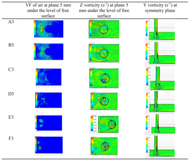
The main aspect of this research is to examine the possibilities of this commercial code to visualize the air entrainment or to detect the ability of identifying the free surface vortices. Visualizing air entrainment is easy: volume fraction (VF) of air or water can be drawn in different cut planes as can be seen later in Figure 14. Free surface vortices can be detected by the examination of pressure field, of the Z vorticity in a plane just below the interface, of the isoline of pressure surface near free surface, of the streamlines or of the air cores from free surface.
The steady calculations (A2, B2, C2, D2, E2 and F2) are used as initial conditions for unsteady calculations (A3, B3, C3, D3, E3 and F3). The steady calculations hardly converged for cases A2, B2, C2 and D2. On the contrary the convergence for the cases E2 and F2 is of good quality.
Except for low submergence (case E3), all cases lead to unstable results, whatever the turbulence model is.
For unsteady calculations, considering the time taken by a particle to go from the inlet to the center of the bellmouth in a straight way, as a characteristic time T (2,5 s for Qm=18 kg/s and 1.67 s for Qm=24kg/s), a total time of 10 s has been chosen for all cases. The time step is 5. 10-3 s.
The unsteady calculations lead to best convergences than steady calculations (residuals less than 1e-5) for the two turbulence models. The two turbulence models give unsteady and unstable results, except case E3, as it can be seen in Figures 10, 14 and 15.
For the reference geometry and the reference mass flow rate (cases A3 and C3), the calculations with k- turbulence model (A3) don’t really conduct to air entrainment. For the k- omega turbulence model, the examination of volume fraction of air at 5 mm under the level of free surface (Figure10) points out the birth of swirls but air entrainment was not pointed up. The examination of Z-vorticity in the same plane and the examination of streamlines confirm this tendency. But the streamlines don't prove air cores occurrences.
For the reference geometry, but with higher mass flow rate (1.5*initial mass flow rate), the k-
model doesn’t really show air entrainment by the examination of volume fraction of air (Figure 10). However, streamlines coming from the center of free surface vortices point up air cores (Figure 11). The air cores can be characterized by the strong density of loops as it can be seen in Figure 11. Unfortunately, the examination of isoline of pressure surface doesn't prove it.
VF of air at plane 5 mm under the level of free
surface
Z vorticity (s-1) at plane 5 mm under the level of free
surface Y vorticity (s-1) at symmetry plane A3 B3 C3 D3 E3 F3
Figure 10. Two-phases model results at time t=6s
The k- turbulence model point up air entrainment as can be observed in Figures 12, 13 and 14. Figure 12 shows the air core. In Figure 13 the beginning of the air core can be detected by the isoline of pressure surface. And finally Figure 14 points up the unsteady state of the vortex. The cut plane, in which air entrainment can be observed, allows detecting the location of a part of the vortex. All indicators of all entrainment are in good agreement. The magnitude of air core is greater in case of k-
So increasing the mass flow rate increase the probability of air entrainment as it has been demonstrated by the two turbulence models. Furthermore the behavior of water in sump pump is highly unsteady, unstable and intermittent. This conclusion wasn't drawn by our experimental results but was already published by other authors [16].
Figure 11. Air cores, case B3,
reference geometry, k-turbulence model,
Qm=24 kg/s, t=10 s
Figure 12. Air cores, case D3,
reference geometry, k-turbulence model,
Qm=24 kg/s, t=5.35 s
Figure 13. Air cores, case D3,
reference geometry, k-turbulence model, Qm=24 kg/s, t = 5.35 s
T=3.85 s T=4.35 s T=4.85 s T=5.35 s
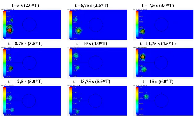
Figure 14. two phases model : air entrainment observed for the D3 model (k- turbulence model,
Qm=24 kg/s)
t =5 s (2.0*T) t =6,75 s (2.5*T) t = 7,5 s (3.0*T)
t = 8,75 s (3.5*T) t = 10 s (4.0*T) t =11,75 s (4.5*T)
t = 12,5 s (5.0*T) t = 13,75 s (5.5*T) t = 15 s (6.0*T)
(k-turbulence model)
The time chosen to observe phenomenon seems to be too small: these first results showed that the behavior of water is highly unsteady and no real periodicity appears. For the last cases the observation time was increased to 15s. For lower submergence and the reference mass flow rate, the two models allow the detection of air entrainment. On the contrary of the results of previous cases, the k-
turbulence model leads to symmetric results which are in good agreement with our experimental results (Figures 16 to 18). The k- turbulence model gives asymmetric and unstable results as it can be seen in figure 15. During the first five seconds, the two turbulence models seem to give some equivalent results. After then the k- turbulence model leads to intermittent results. The magnitude of one of the two air cores increases as the magnitude of the other increases but this phenomenon doesn't seem to be periodic. The potential air entrainment is detected by the visualization of air cores, of is pressure plane and streamlines from free surfaces (Figures 19-21). The VF of air doesn't allow this visualization probably due to the unstable position of air cores.
Figure 16. Air core
k-turbulence model at t=15 s
Figure 17. Iso pressure k-
turbulence model at t=15s
Figure 18. Streamlines from
free surface k- turbulence model at t=15 s
Figure 19. Air core k-
turbulence model at t=15 s
Figure 20. Iso pressure k-
turbulence model at t=15 s
Figure 21. Streamlines from
free surface k- turbulence model at t=15 s
5. Conclusion
The present study shows the ability of a commercial code to predict the two phase flow behaviour inside a pump sump with good agreements with experimental investigations. Unless one specific result, this study allows establishing some rules that must be applied regarding the ability of Star CCM+ code to predict air entrainment in sump pump.
Unless one specific result, all others prove that the flow basic characteristics in the sump pump are highly unsteady, unstable and intermittent whatever the turbulence model is.
Unsteady two phases flow model allows visualizing the behaviour of water in sump pump taking account the real influence of free surface. The air entrainment visualization seems to be easy by using the volume of fluid of air. But this parameter can only be caught in defined cut planes. The great difficulty is the unsteady position of the air core making the choice of cut planes not so easy.
Unsteady numerical results also show that the strength of the two vortices is not equal and changes depending on time. One vortex grows up and at the same time the second one decreases; this
phenomenon seems to have a specific frequency based on the mean stream velocity and on the diameter of the tube.
It seems that the potential air entrainment begins for the submergence equal to 1.2D (reference case) for the reference mass flow rate for the k- turbulence model.
1. Nomenclature
b1 b2 d D e Fr g H h hb l Qm Red RehPipe left wall distance [m] Pipe right wall distance [m] Pipe intake interior diameter [m] Baffle intake interior diameter [m] Pipe back wall distance [m]
Froude number for the pipe submergence (=V/(gd)1/2)
Acceleration due to gravity [m/s2]
Water level in the sump-pump [m] Submergence depth for the pipe [m] Baffle height [m]
Pipe back side distance [m] Mass flow [kg/s]
Reynolds number in the pipe (=VD/) Reynolds number in the sump (=Qm/h)
T U V W We z ν ρ σ ω 1 2 Characteristic time (s)
Mean velocity in the sump [m] Mean velocity in the intake pipe [m] Pump-sump width [m]
Weber number (=V2D/)
Clearance distance from floor [m] kinematic viscosity [m2/s]
Water density. [kg/m3]
Coefficient of surface tension [N/m] Specific dissipation rate [s-1]
Subscripts for level free surface inside sump
Subscripts for level free surface inside pipe
References
[1] Bayeul-Lainé A C, Bois G, Issa A 2010 Numerical Simulation of flow field formed in water-pump sump 25th IAHR Symp. on hydraulic Machinery and Systems september 20-24 Timisoara Romania
[2] Issa A 2009 Etudes hydrauliques de l’influence des géométries des basins sur l’alimentation des pompes Ph. D Thesis Arts et Metiers PARISTECH Ecole doctorale.
[3] Issa A, Bayeul-Lainé AC, Bois G. 2008 Numerical Simulation of Flow Field Formed in Water Pump-Sump 24h IAHR Symp. Hydraulic Machinery Systems october 27-31 Brazil.
[4] Issa A, Bayeul-Lainé AC, Bois G 2009 Numerical study of the influence of geometrical parameters on flow in water sump-pump 14th International Conference on Fluid Flow Technologies September 9-12Budapest Hungary
[5] Constantineascu G and Patel V C 1998 Numerical Model for Simulation of Pump Intake Flow and Vortices J. of hydraulic Engineering. Div ASCE vol 124 123-134
[6] Nakato T 1988 Hydraulic-Laboratory Model Studies of the Circulation-Water Pump-Intake Structure, Florida Power Corporation, Crystal River. Units 4 and 5 IIHR Rep. No.320, Iowa Inst.of Hydr. The Univ of Iowa. Iowa City.
[7] Nakato T 1989 A Hydraulic-Model Study of the Circulation-Water Pump-Intake Structure Laguna Verde Nuclear Power Station, Unit. 1, Commission Federal De Electrcidad. IIHR Rep. No.330, Iowa Inst.of Hydr. The Univ of Iowa. Iowa City
[8] Nakato T 1990 A Hydraulic-Model Study of the Proposed Pump-Intake and Discharge Flume Crystal River Cooling-Tower Project IIHR Rep. No.339 Iowa Inst.of Hydr. The Univ of Iowa. Iowa City
[9] Nakato T 1991 Improvement of pump-approach flows A hydraulic model study of Union Electric’s Meramec plane circulating-water pump intakes IIHR Rep. No 348 Iowa Inst of Hydro Res. The Univ of Iowa, Iowa City, Iowa
[10] Ettema R and Nakato T 1990 Hydraulic-Model Study of the Circulation-Water and Essential-Service-Water Pump-Intake structures: Korea Electric Power Corporation Yonggwag Station, Units 3 and 4 IIHR Limited Distribution Rep. No.33 Iowa Inst.of Hydr. The Univ. of Iowa. Iowa City. Iowa.
[12] Anwar HO and Amphlett M B 1980 Vortices at Vertically in Vertex Intake J. Hydr. Res., 18(2) 123-134
[13] Daggett LL and Keulegan G H 1972 Similitude Conditions in Free Surface Vortex Formation J. Hydr. Div. ASCE. 100(11) 1565-1580
[14] Matsui J, Kamemoto K, and Okamura T 2006 CFD Benchmrak and a Model Experiment on the Flow in Pump Sump Proc. of 23th IAHR Symp. October 17-21Yokohama 110-16
[15] Isbasoiu EC, Muntean T, Safta C A, Stanescu P 2005 Swirling flows in the suction sumps of vertical pumps, theoretical approach Workshop on vortex dominated flows June Timisoara Romania pp 17-22
[16] Lucino C, Gonzalo Dur SL 2010 Vortex detection in pump sumps by means of CFD , XXIV latin American congress on hydraulics November Punta del este Uruguay
[17] Shulka Kshirsagar JT 2008 Numerical prediction of air entrainment in pump intakes Proc. of the24th int. pump users Symp. pp 29-33
[18] Shih, Liou WW, Shabbir A, Yang Z and Zhu J 1995 A New k- Eddy Viscosity Model for High Reynolds Number Turbulent Flows: Model, Development and validation Computers and Fluids Vol 24 No 3 pp227-238
[19] Rodi W 1991 Experience with Two-Layer Models Combining the k-e Model with a One-Equation Model Near the Wall 29th Aerospace Sciences Meeting January 7-10 Reno NV AIAA 91-0216
[20] Menter FR 1994 Two-equation eddy-viscosity turbulence modeling for engineering applications AIAA Journal 32(8) pp. 1598-1605