Science Arts & Métiers (SAM)
is an open access repository that collects the work of Arts et Métiers Institute of Technology researchers and makes it freely available over the web where possible.
This is an author-deposited version published in: https://sam.ensam.eu Handle ID: .http://hdl.handle.net/10985/10919
To cite this version :
Jean-Philippe BIANCHI, Etienne BALMES, Mac Lan NGUYEN-TAJAN - Dynamic stress prediction in catenary wires for fatigue analysis - In: IAVSD, Autriche, 2015-08 - IAVSD - 2015
Any correspondence concerning this service should be sent to the repository Administrator : [email protected]
1 INTRODUCTION
Today, the main criterion used to determine the Contact Wire (CW) replacement is its wear. On high speed lines, due to their specific geometries, the wear ratio is very small compared to clas-sical lines so that the CW lifespans due to wear is more than 50 years. The traffic is very im-portant on French high speed lines: an average of 150 000 pantographs are circulating on a giv-en line each year. As a consequgiv-ence, the number of load cycles that a CW will giv-endure during its lifespan is very high, so the fatigue process must be taken in account to avoid fractures of the catenary CW, leading to traffic disruptions, passengers’ dissatisfaction and huge induced costs for SNCF.On-line crack detection is very difficult so numerical simulation can help target criti-cal areas where crack is likely to occur, but also to understand risk factors, and estimate when the crack can occur. This paper presents the fatigue simulation tools developed within the OS-CAR software.
OSCAR is the software used by SNCF and developed by SDTools to model the dynamic inter-action between pantograph and catenary [Massat 2015]. This package developed within the Structural Dynamics Toolbox for MATLAB [SDTools 2015] is a well validated tool that is used for design and validation of catenaries. The catenary is described using the finite element meth-od, meshing each wire with beam elements. A full nonlinear static taking in account beam pre-tensions and dropper unilaterality is first computed. Then a nonlinear dynamic computation is performed with a sliding contact between one or more pantographs (described from the simplest 3 lumped mass model to more accurate flexible multibody models), leading to the dynamic dis-placements of all the contact wire nodes.
Stress could be evaluated from the beam model using the Euler-Bernoulli formalism. But the uniaxial nature of beam stresses is insufficient and crack initiation typically occurs in transition areas (claws, …), where the validity of a beam model can clearly be doubted. A full volume meshing of a CW section (~1 km) is not realistic because of the associated model size, so that a volume mesh is included in the beam mesh of the CW only on a short studied area. The process
Dynamic stress prediction in catenary wires for fatigue analysis
J.P. Bianchi
SDTools, Paris, France
E. Balmes
SDTools & Arts et Métiers ParisTech, PIMM, Paris, France
M.-L. Nguyen-Tajan
SNCF Innovation & Research department, Paris, France
ABSTRACT: Fatigue cracks in the contact wire are a possible cause of fracture which can in-duce huge costs. Fatigue study is thus of a great interest but requires an accurate computations of stress distributions. OSCAR is a SNCF software used to study coupled pantograph / catenary dynamics. It is based on Euler-Bernoulli beam meshes. This formalism is accurate to study the catenary displacements, but is not sufficient to compute multi-axial stresses, in particular in parts that can concentrate stresses such as the junction claws. This paper details and illustrates the strategy developed to compute a full multi-axial transient stress field, in any point of the contact wire. The dynamic displacement computed by OSCAR is expanded and combined with a precise nonlinear static state of a mixed model of beams and volume elements.
to obtain proper 3D stresses from this model is first described. One then introduces fatigue crite-ria based on the Dang-Van theory. Finally sample results are shown for the study of a junction claw.
2 TRANSIENT STRESS COMPUTATION IN A VOLUME MESH IN OSCAR
The general method, detailed in this section and summarized in the Figure 1, aims at computing stresses at any point of a CW. Two models are defined from OSCAR standard model of catena-ry which combines beams, bar and mass elements. The first mixed model, detailed in section 2.1, combines the OSCAR model and volume mesh of an area of interest (studied area). It is used to compute 3D static stresses, detailed in section 2.2, and an expansion basis detailed in section 2.3. The second model is a standard OSCAR model refined or adapted to have a number of coincident nodes with the mixed model. This adapted model is used to compute the dynamic displacements that will be expanded to estimate the dynamic part of the 3D transient stresses.
Figure 1. General process for stress computations. 2.1 Catenary meshing
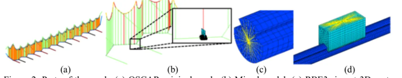
The first step of the considered strategy is to generate a standard OSCAR mesh (Figure 2a) that is composed of pre-stressed beams and mass elements. Then an area of interest, where fatigue study will be performed, is meshed in detail using volume elements: a CW segment of a few meters and all claws connected to this segment (junction claw, dropper claw…). The volume mesh is inserted in the beam mesh replacing beams (Figure 2b), connecting the CW volume mesh extremities to adjacent beams through rigid link rings (Figure 2c), and the dropper claws to the dropper through RBE3 ring (Figure 2d). This results in the mixed model of Figure 1.
(a) (b) (c) (d)
Figure 2. Parts of the mesh. (a) OSCAR original mesh. (b) Mixed model. (c) RBE3 ring at 3D part ex-tremity. (d) Dropper claw connection.
The 3D studied area is generated by automated meshing of wire and claw sections followed by an irregular extrusion. The resulting elements are pentahedra. Element size is varying in CW
section around 1 mm, and the extrusion step is typically 2 mm. The length of the 3D studied ar-ea varies from 1.5 to 2 m lar-eading to model sizes in the 500 000 to 700 000 DOF range.
The adapted model is generated from the initial OSCAR model, and the mesh of the studied area. The adaptation consists mainly in refining the beams in the studied area to have coincident nodes on the neutral fiber of the CW. The claws that are typically defined by masses are also re-placed by more accurate models. This adaptation is a key to obtain a correct expansion for the dynamic displacements: the adapted model must give an accurate beam/bar/mass representation of the mixed model.
2.2 Static 3D stresses
The second step is a nonlinear static resolution of the mixed model taking in account gravity, pre-stress in beam elements and full geometric non-linearity in the volumes. At each iteration step, one considers residuals in the “1D” (beam/bar/mass elements) and “3D” parts (volume mesh of the studied area).
In the 1D part wires the tension is adjusted leading to a change in the tangent stiffness in beam elements. This change in tangent stiffness is the only effect of geometric non-linearity. Unilateral stiffness in the droppers is also accounted for even though it is usually not activated in the static behavior. The 1D residual is thus given by
{ ( )} = [ ( )]{ } − F + − { ( )} (1)
In the volumes, the full Green-Lagrange strain
{ } = FF − I = ((I + ∇u)(I + ∇u) − I) (2)
is computed and is related to the Piola-Kirchoff stress by an elastic law
{ } = λTr(e)I + 2μe (3)
and leads to the 3D residual
{ ( )} = ∫ . − ∫ ( ) : (4)
The nonlinear solution then seeks to minimize residuals through iterations on . Linear con-straints associated with the beam/volume connections are handled by elimination. One starts from a zero state and considers displacement increments
{ } = { } − { } = [ ][ ( )] { ( )} (5)
that verify the constraints. It is noted that the current computation does consider constraints in the nominal geometry, when updating these constraints to account for the large transformation might be needed.
In some configurations, convergence was difficult. Solutions to obtain convergence involved application of tension in multiple steps, adjustment of tolerances, Jacobian updating, tuning of line-search parameters. Number of iterations can be important. A typical computation time for 3D static and expansion matrix is 2 hours.
2.3 Dynamic 3D stresses
Jacobian reassembly and factorization, while reasonably fast (320 s for a light 350 000 DOF model), is incompatible with transient simulations where the moving load of the pantograph must absolutely be accounted for as will be shown later in the paper. The passage of the panto-graph over the 1-2 meter 3D segment would require at least 250 time steps at 300 km/h (mini-mum because the convergence of such a computation will certainly need a time step far much lower than the 1D computation time step of 1e-4 s): that corresponds to more than 20 h. As it would be difficult to perform simulation on the mixed model only when pantograph is under the studied area, and then go back to 1D model elsewhere, the simulation of the train passage on a full section would take a huge amount of time, which is unrealistic. Besides geometry transition
between beam and volume meshes would be a very complex task (contact strategy, wave reflec-tions problems...) in the dynamic problem.
The proposed solution is thus to expand the response of the adapted model. The resolution of the adapted model transient is a standard OSCAR run, which is using a fixed Jacobian strategy, and takes about 12 min for a full section. The simulation uses a time step of 1e-4 s in a New-mark implicit scheme with Newton iterations, and accounts for beam pretension, dropper unilat-erality, and pantograph moving contact.
Static and dynamic solutions of the adapted mesh lead to transient solutions
( , ) = , ( ) + ( , ) (6)
decomposed in a static part , ( ) and a dynamic fluctuation ( , ). It is then assumed that
the full 3D response can be decomposed into a nonlinear static part and a linearized dynamic so-lution
( , ) = , ( ) + [ ]( ( , )) (7)
where recovery of the 3D displacements from beam motion to full 3D response is obtained us-ing the static reduction/condensation basis [ ] [Guyan 1965].
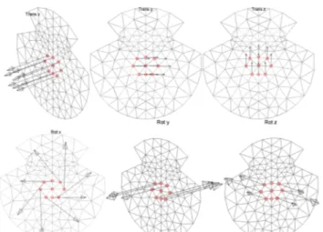
Since the rotations are not present in volumes, a strategy to couple beam rotation DOFs and volumes is needed. One thus considers six independent loads, shown in Figure 3, on a ring of nodes around the neutral axis. From these loads, one builds a series of static deformation shapes of the mixed model such that observation of translations and rotations on the adapted model mesh part correspond to unit translations and rotations, thus leading to the reduction basis.
Figure 3. Unit loads corresponding to 6 interface DOFs of Guyan condensation. Top: translations, bottom: rotations.
The Guyan condensation matrix [T] can be quite large. For example, for a simple case where study part is 2 m long, extruded with 2 mm step, there are 1000*6 master DOFs on the neutral fiber and 700 000 DOFs in the volume mesh. That leads to an expansion matrix of approximate-ly 30 GB. This matrix takes a lot of memory so that it is stored out of core.
Stresses are linearly related to displacements. It is thus possible to build an observation equa-tion for stresses at specific posiequa-tions and to use the expansion (7) to obtain
( , ) = [ ] , ( ) + ( , ) = , + [ ] ( , ) (8)
where the static stress , and the stress observation matrix [cT] can be precomputed so that the application of (8) has a very low cost.
Rich parametric studies on train configuration can thus be performed with a single time consum-ing 3D run. Examples of parameters are pantograph properties or types, distance between pan-tographs. Their impact on the fatigue criticality can be assessed. Results of such a study are pre-sented in section 3.4.
3 APPLICATION
This section illustrates the proposed method. Section 3.1 summarizes the principles used to go from stress predictions to fatigue analysis. Section 3.2 details the behavior for a junction claw. Section 3.3 justifies the need to compute full multi-axial stresses. Section 3.4 illustrates how this tool can be used to hierarchize pantograph aggressiveness in terms of fatigue damages caused to the CW.
3.1 Principle of crack prediction
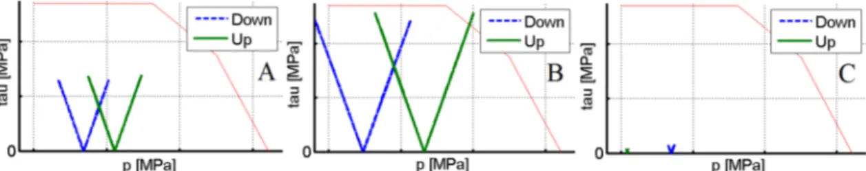
The computation of the transient stress field is meant as input to a fatigue prediction model, based on the Dang-Van theory, with enrichment and extensions. The fatigue limit domain of the common copper alloy is modeled with a multi-slope Dang Van criterion, as shown in Figure 4. The material characteristics were identified thanks to fatigue tests performed by SNCF on small specimen subjected to cyclic bending loads. In the Dang Van histogram (mesoscopic shear stresses according to hydrostatic pressure), the cyclic stresses path of any point of the CW can be plotted. The criticality of a given cycle due to a train passage is quantified by a scalar called criticality (“Cd” in the figures). This criticality Cd has been directly linked to an expected lifespan before crack initiation via an innovative method detailed in a later publication.
A negative Cd means that there is no criticality of the studied cycle, according to the number of cycles chosen to build the unlimited endurance domain (in this study, five million cycles have been retained). In Figure 4, the red (+) and blue (triangle) cycles corresponding to points located at the center and the bottom of CW have negative Cd. A positive Cd implies that the risk of fa-tigue needs to be taken in account. This is the case of the point at top of the CW in Figure 4.
Figure 4. Dang-Van cycles at 3 points of the CW section : top (green plain line with stars), center (red plain line with triangles) and bottom (blue dashed line with + markers).
3.2 Detailed behavior for a junction claw
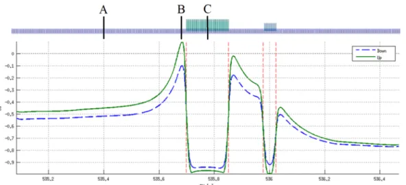
We consider here, as an example, the case of junction claw, on a French high speed catenary. The train circulates at a speed of 300 km/h and has only one pantograph. The criticality diagram representing the criticality on the upper line and on the lower line of the CW against the position on the studied area given in Figure 5. Criticality is maximum about 1.5 cm before the junction claw, on the top of the CW.
Figure 5. Criticality on a line on the top (green plain line) and on the bottom of the CW (blue dashed line) against position in the line (PK). Claws are delimited by vertical red dashed lines (left: junction claw, right: dropper claw).
Figure 6 shows more precisely the evolution of the axial stresses σxx in the studied area. In the time/space domain, the junction and dropper claws are shown by horizontal dashed lines. The pantograph position is represented by oblique dashed line. Waves that come before pantograph are visible but low. The point where stresses are the most important is located few centimeters before the junction claw and reached a little after the pantograph passage. Under the claw, stresses are low with the highest tension due to the wave arriving before the pantograph.
Displacements of the CW are shown in Figure 7. The junction claw is very stiff and has a mass of more than 1 kg so its inertia is important. That explains why the maximum stress is lo-cated before the junction claw: the bending of the CW generated by the pantograph approach is blocked before the claw is raised by the pantograph.
Figure 6. Contour color map of CW axial stresses at the upper line of the studied area (left) and at the lower line (right).
Figure 7. Displacement for different time steps during train passage.
Figure 8 shows a zoom of the transient σxx stresses at the 3 positions A, B and C (see Figure 5), at the top and the bottom of CW.
At points A and B, before the train passage, some waves induce low stress variations in the CW. When the train passes under a given point of the CW, a strong short stress peak can be ob-served at its top and bottom. Stress oscillations quickly decrease so that the dimensioning part of the stress signals is localized around the time of the train passage. To avoid missing the peak, the nominal 1.2 ms time step is divided by 100.
A 20 000 N tension is applied to the CW extremities. For a section of 151.5 mm2, the mean σxx stress is 132 MPa. Under gravity load, the CW is sagging, the top is compressed while the bottom is tensed and thus shows a higher stress. When pantograph passes and applies a vertical load around 180 N, the CW bends in the direction opposite to sag and tension increases at the top and decreases below. Figure 8 shows that maximum stresses are almost opposed to mini-mum stresses around the mean value equal to 132 MPa: due to the slots of CW, its neutral fiber is closer to its bottom than to its top so that during a same bending, σxx stress increases more at the top than it decreases at the bottom.
Point C is rather particular because it is located under the junction claw. The junction claw is clamping the CW, without sliding, so that a part of the tension of the CW is passing through the claw: static σxx stress is about 40 MPa at the top of CW and 100 MPa at the bottom of CW. When the train passes under the junction claw, there is almost no bending of the CW because the claw is very stiff, so that the stress peak is very low.
Figure 8. Transcient stresses at the 3 positions A, B and C, at the upper point and the lower point of CW. Figure 9 shows the Dang-Van paths at the top and the bottom of the 3 positions A, B and C corresponding to the stresses displayed Figure 8. The Dang-Van paths must be compared to the Dang-Van endurance limit to determine the criticality of corresponding cycles. The only critical cycle is at the top of the CW at position B. Other cycles are not critical (no risk of crack initia-tion).
At positions A and B, the Dang-Van path at the bottom of the CW has a lower hydrostatic pressure than at the top. This is due to the fact that mean stress in a cycle is lower at the bottom than at the top: when the pantograph passes, the increase of stress occurs at the top whereas stress decreases at the bottom of the CW. Besides stress increase is more important at the top of the CW than the stress decrease at the bottom. That is why upper point is more critical in simu-lations than lower point. In reality stress crack may occur at the bottom of the CW. That can be explained by neglected phenomena in simulations, such as for example electric arks due to pan-tograph CW contact losses, shocks or friction with panpan-tograph, wear....
At position C, the stress variations are very low because of the claw stiffness that prevents CW from deforming too much. There is no risk of crack initiation at this position.
Figure 9. Dang-Van paths at the 3 positions A, B and C, at the upper point and the lower point of CW. 3.3 Discussion on 3D/beam stresses relation
A full dynamic computation can be performed within the beam model in about ten minutes and transient axial stresses in Euler-Bernoulli formalism can be easily computed. In this section the interest of a full 3D stress field computation is illustrated.
The first argument to compute full 3D stress field is that Saint-Venant insures good validity of beam theory in area far enough from singularities. In our case the stresses computed are only valid few centimeters from the claws. But it has been shown by full 3D computations that these areas are critical and consequently of a main interest.
As an illustration, we compare the σxx amplitudes at the top of the CW during a train passage computed in the Euler-Bernoulli formalism and computed from the full 3D process detailed in this paper. Outside singularity areas, the two amplitudes are really close, but near the claw it is no longer the case. Figure 10 compares the two amplitudes at the level of a dropper claw: the beam stress is not regular whereas 3D stress evolution is more progressive. Differences are clearly visible.
Figure 10. σxx amplitudes at a dropper claw level, on a CW upper line. The axial component of the full 3D
computation is the dashed line and the plain line is the beam computation.
Due to stagger and Z/Y coupling, there are non axial stresses in the catenary (even if they are low), as illustrated Figure 11. At the point C, under the junction claw, there is a -30 MPa σyy stress component that is due to the tightening load.
Figure 11. Non axial stresses at positions A, B and C.
The main stress is however σxx. To select the relevant points within the section, Figure 12 displays σxx stresses map at point B and C sections. The deformation is mainly caused by verti-cal bending of the CW that justifies considering only CW top and bottom line observations. At point C, junction claw is taking a part of the CW tension because of adherence, so that σxx is lower at the top than at the bottom. We see also on the picture the 2 points where tightening load is applied (σxx stress locally negative).
Figure 12.Stress distribution. Left: critical point (point B). Right: under the junction claw (point C). 3.4 Junction claw:Pantograph damages caused to the catenary
CW cracks under a junction claw have been reported. Those claws are heavy and stiff so they induce important dynamic stresses when the pantograph is passing. In section 3.2 a nominal case of a junction claw was studied in detail. In particular Figure 5 showed the criticality on the upper and lower line of the CW: there is a visible critical point before the junction claw, on the top of the CW. Since fatigue damage is related to criticality, it is obviously interesting to com-pare the effect of different pantographs, in different setups, in order to assess the induced dam-age. This will allow the use of fatigue criteria in the selection of pantograph configurations for networks that now tend to have multiple operators.
Two realistic pantographs, named 1 and 2 in the paper are considered. Simulations are per-formed on a standard section of the high speed line that connects Paris to Le Mans. A junction claw is added near the last dropper of a span at the middle of the section. Each train is composed of a unique pantograph. A simulation is performed for different pantographs and mean contact forces (from 70 N to 300 N by 10 N steps) for a train speed of 300 km/h.
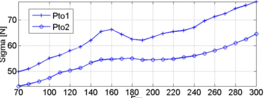
Figure 13 shows the maximum of criticality around the junction claw, on the top and the bottom line. Pantograph 1 is clearly more aggressive than pantograph 2 in terms of fatigue whatever the mean contact force Fm. The impact of Fm on criticality is also more important in the case of pantograph 1. Criticality is globally increasing in both cases with Fm. Some mean contact forces are clearly more damaging: for example there is a peak of criticality for Fm=150N for pantograph 1.
Figure 13. Maximum of criticality around the junction claw, at CW top (green dashed line) and bottom (blue dashed line) against mean contact of pantograph (Fm 70 N to 300 N). Pantograph 1 (+) and 2 (o).
The standard deviation of the contact force on the whole section can be considered as an indi-cator of current collection quality. Figure 14 shows that pantograph 2 is much better regarding the current collection than pantograph 1. The peak in fatigue aggressiveness, observed in Figure
13 around Fm=150 N, can also be found as a peak in the contact force standard deviation. Fa-tigue aggressiveness and beam dynamics are thus clearly related.
Figure 14. Standard deviation of unfiltered contact force on the whole section. Pantograph 1 (+) and 2 (o).
4 CONCLUSION
The fatigue module developed and detailed in this paper gives access to multi-axial stresses at any point of the CW. Computing the multi-axial transient stresses gives more precision on the axial component σxx that would be really approximated near the singular points, junction claws in particular, if computed from the standard beam models. The multi-axial transient stress field can be applied for advanced fatigue theories, such as the Dang-Van method that has been used and extended to compute the number of years before a crack is likely to occur. This “time to live” indicator will be the object of further publication.
A main result of this study was the confirmation that claws are the most critical points in terms of CW fatigue known this day. Details about the behavior in this area were given in the paper.
The proposed tool seems practical to help define maintenance strategies. It indeed allows de-tection of critical points and classification of the impact of different operating conditions. Con-tact force and damage were found to be strongly correlated. Using inline conCon-tact force meas-urements to build indicators of critical areas thus seems an interesting perspective.
REFERENCES
Balmes, E. & Bianchi, J.-P. & Leclère, J.-M. & Bobillot, A. & Massat, J.-P. 2015. OSCAR 2.0 User’s guide.
Massat, J.-P. & Balmes, E. & Bianchi, J.-P. & Van-Kalsbeek, G. 2015. OSCAR statement of methods. Vehicle System Dynamics.
SDTools. 2015. Structural Dynamics Toolbox & FEMLink User’s guide. SDTools, www.sdtools.com. Guyan, R.J. 1965. Reduction of Mass and Stiffness Matrices. AIAA Journal volume 3.
Nguyen-Tajan M.-L. & Mai S.H. & Massat J.-P. & Avronsard, S. & Banting J. & Bianchi J.-P. & Mai-tournam, H. 2013. Fatigue crack initiation risk analysis and crack propagation modelling in the catenary contact wire of high speed lines. WCRR.