Balancing cost and flexibility in Supply Chain

HAL Id: tel-02125192

https://pastel.archives-ouvertes.fr/tel-02125192

HAL is a multi-disciplinary open access archive for the deposit and dissemination of sci-entific research documents, whether they are pub-lished or not. The documents may come from teaching and research institutions in France or abroad, or from public or private research centers.

L’archive ouverte pluridisciplinaire HAL, est destinée au dépôt et à la diffusion de documents scientifiques de niveau recherche, publiés ou non, émanant des établissements d’enseignement et de recherche français ou étrangers, des laboratoires publics ou privés.

Balancing cost and flexibility in Supply Chain

Etienne Gaillard de Saint Germain

To cite this version:

Etienne Gaillard de Saint Germain. Balancing cost and flexibility in Supply Chain. Dynamical Systems [math.DS]. Université Paris-Est, 2018. English. �NNT : 2018PESC1113�. �tel-02125192�

École doctorale MATHÉMATIQUES ETSCIENCES ETTECHNOLOGIES DE L’INFORMATION ET DE LACOMMUNICATION

T

HÈSE DE DOCTORAT

Spécialité : Mathématiques

Présentée par

Etienne G

AILLARD DE

S

AINT

G

ERMAIN

DOCTEUR DE L’UNIVERSITÉPARIS-EST

B

ALANCING COST AND FLEXIBILITY

IN

S

UPPLY

C

HAIN

Soutenance le 17 décembre 2018 devant le jury composé de :

Mme Nadia B

M. Jean-Philippe G

Mme Safia K

-S

Mme Céline G

M. Fabrice B

M. Vincent L

Remerciements

Ces trois années de thèse écoulées, je prends conscience de la chance que j’ai eu d’être entouré par chacun d’entre vous.

Je tiens tout d’abord à remercier mes directeurs de thèse Vincent Leclère et Frédéric Meunier. Vous avez su me faire grandir personnellement et scientifiquement, m’aiguiller et m’offrir de l’autonomie sans cesser de veiller sur moi. Surtout, je vous suis reconnaissant pour avoir toujours su me rassurer, calmer mes doutes et me permettre d’effectuer ma thèse dans les meilleures conditions.

J’adresse mes sincères remerciements à Jean-Philippe Gayon et Safia Kedad-Sidhoum pour avoir accepté de rapporter ma thèse et m’avoir montré comment améliorer ce manuscrit. Je remercie également Nadia Brauner et Céline Gicquel d’être présentes pour ma soutenance.

Je souhaiterais adresser un remerciement particulier à Fabrice Bonneau, Directeur Général d’Argon Consulting pour l’intérêt des sujets proposés, sa disponibilité malgré son emploi du temps chargé et sa volonté d’investir et de s’investir dans cette recherche malgré les contraintes industrielles. Comprendre les enjeux humains qui se cachaient dernière les mathématiques fut un réel plaisir. Je remercie également toutes les personnes que j’ai pu côtoyer à Argon Consulting : celles qui m’ont transmis leur passion et leur connaissance de la Supply Chain, les fonctions supports sans qui le quotidien ne serait pas si simple, ceux avec qui j’ai pu tisser des liens d’amitié et particulièrement les membres de l’OSS 117.

Je remercie également tous les chercheurs du CERMICS pour leur disponibilité et en particulier Jean-Philippe Chancelier sans qui l’informatique aurait été beaucoup plus difficile et Bernard Lapeyre et Julien Reygner pour leur aide sur les probabilités. Je remercie également les doc-torants qui ont su créer un environnement de travail et de détente en toute circonstance. En particulier, je repense à nos conversations surréalistes à des heures tout aussi improbables, à ce séjour en Auvergne et cette “petite ballade” qui aura finalement duré cinq heures et à notre séjour au ski. Enfin, je souhaiterais adresser un remerciement tout particulier à Isabelle Simunic, la Secrétaire Générale du CERMICS. Arrivé petit stagiaire en césure, tu m’as accueilli quelques semaines dans ton bureau, pendant lesquelles ta réserve de spéculoos a grandement diminuée. Tu t’es toujours pliée en quatre pour nous rendre la vie facile et tu nous montrais toujours ta bonne humeur malgré les difficultés de ton travail.

Je remercie également mes amis qui sont là aujourd’hui et qui me rendent la vie si agréable, que ce soit lors des sorties ou des soirées Donjons et Dragons. Je me libère également aujourd’hui de toute blague sur mon statut étudiant.

Finalement, mes derniers remerciements vont à ma famille. Merci Maman pour ton soutien, ta présence ton écoute. Merci d’être aussi rock-and-roll. Merci à mes frères et sœurs, Aleth, Louise, Simon et Matthias. Merci d’être si déjantés et motivés pour tout (même le pire !) et de supporter ma maniaquerie. Merci à Natacha, la fiancée de Louise, pour nos parties de tennis hebdomadaires et pour être devenue ma troisième sœur. Enfin, tu n’es pas présent aujourd’hui malgré ton importance : merci Papa. Tu as été là à toutes les étapes de ma vie et particulièrement pendant cette thèse. Pendant deux ans et demi, j’ai pu avoir cette relation privilégiée avec toi lorsque je vivais sous ton toit. Tu remplissais tous les rôles : le père, le colocataire, l’ami, le confident. Si cette thèse a pu si bien se dérouler, je te le dois en grande partie.

Abstract

This thesis develops optimization methods for Supply Chain Management and is focused on the flexibility defined as the ability to deliver a service or a product to a customer in an uncertain environment. The research was conducted throughout a CIFRE agreement between Argon Consulting, which is an independent consulting firm in Supply Chain Operations and the École des Ponts ParisTech. In this thesis, we explore three topics that are encountered by Argon Consulting and its clients and that correspond to three different levels of decision (long-term, mid-term and short-term).

When companies expand their product portfolio, they must decide in which plants to produce each item. This is a long-term decision since once it is decided, it cannot be easily changed. More than an assignment problem where one item is produced by a single plant, this problem consists in deciding if some items should be produced by several plants and by which ones. This is motivated by a highly uncertain demand. So, in order to satisfy the demand, the assignment must be able to balance the workload between plants. We call this problem the multi-sourcing of production. Since it is not a repeated problem, it is essential to take into account the risk when making the multi-sourcing decision. We propose a generic model that includes the technical constraints of the assignment and a risk-averse constraint based on risk measures from financial theory. We develop an algorithm and a heuristic based on standard tools from Operations Research and Stochastic Optimization to solve the multi-sourcing problem and we test their efficiency on real datasets.

Before planning the production, some macroscopic indicators, such as the quantity of raw materials to order or the size of produced lots, must be decided at mid-term level. Continuous-time inventory models are used by some companies but these models often rely on a trade-off between holding costs and setup costs. These latters are fixed costs paid when production is launched and are hard to estimate in practice. On the other hand, at mid-term level, flexibility of the means of production is already fixed and companies easily estimate the maximal number of setups. Motivated by this observation, we propose extensions of some classical continuous-time inventory models with no setup costs and with a bound on the number of setups. We used standard tools from Continuous Optimization to compute the optimal macroscopic indicators. Finally, planning the production is a short-term decision consisting in deciding which items must be produced by the assembly line during the current period. This problem belongs to the well-studied class of Lot-Sizing Problems. As for mid-term decisions, these problems often rely on a trade-off between holding and setup costs. Basing our model on industrial considerations, we keep the same point of view (no setup cost and a bound on the number of setups) and

propose a new model. Although these are short-term decisions, production decisions must take future demand into account, which remains uncertain. We solve our production planning problem using standard tools from Operations Research and Stochastic Optimization, test the efficiency on real datasets, and compare it to heuristics used by Argon Consulting’s clients.

Key words: Assignment Problem, Heuristics, Lot-Sizing, Operations Research, Risk Measure, Stochastic Optimization, Supply Chain Management.

Résumé

Cette thèse développe des méthodes d’optimisation pour la gestion de la Supply Chain et a pour thème central la flexibilité définie comme la capacité à fournir un service ou un produit au consommateur dans un environnement incertain. La recherche a été menée dans le cadre d’une convention CIFRE entre Argon Consulting, une société indépendante de conseil en Supply Chain, et l’École des Ponts ParisTech. Dans cette thèse, nous étudions trois sujets rencontrés par Argon Consulting et ses clients et qui correspondent à trois différents niveaux de décision (long terme, moyen terme et court terme).

Lorsque les entreprises élargissent leur portefeuille de produits, elles doivent décider dans quelles usines produire chaque article. Il s’agit d’une décision à long terme, car une fois qu’elle est prise, elle ne peut être facilement modifiée. Plus qu’un problème d’affectation où un article est produit par une seule usine, ce problème consiste à décider si certains articles doivent être produits par plusieurs usines et par lesquelles. Cette interrogation est motivée par la grande incertitude de la demande. En effet, pour satisfaire la demande, l’affectation doit pouvoir équilibrer la charge de travail entre les usines. Nous appelons ce problème le multi-sourcing de la production. Comme il ne s’agit pas d’un problème récurrent, il est essentiel de tenir compte du risque au moment de décider le niveau de multi-sourcing. Nous proposons un modèle générique qui inclut les contraintes techniques du problème et une contrainte d’aversion au risque basée sur des mesures de risque issues de la théorie financière. Nous développons un algorithme et une heuristique basés sur les outils standard de la Recherche Opérationnelle et de l’Optimisation Stochastique pour résoudre le problème du multi-sourcing et nous testons leur efficacité sur des données réelles.

Avant de planifier la production, certains indicateurs macroscopiques doivent être décidés à moyen terme tels la quantité de matières premières à commander ou la taille des lots pro-duits. Certaines entreprises utilisent des modèles de stock en temps continu, mais ces modèles reposent souvent sur un compromis entre les coûts de stock et les coûts de lancement. Ces derniers sont des coûts fixes payés au lancement de la production et sont difficiles à estimer en pratique. En revanche, à moyen terme, la flexibilité des moyens de production est déjà fixée et les entreprises estiment facilement le nombre maximal de lancements. Poussés par cette observation, nous proposons des extensions de certains modèles classiques de gestion de stock en temps continu, sans coût de lancement et avec une limite sur le nombre de lancements. Nous avons utilisé les outils standard de l’Optimisation Continue pour calculer les indicateurs macroscopiques optimaux.

quels articles doivent être produits par la ligne de production pendant la période en cours. Ce problème appartient à la classe bien étudiée des problèmes de Lot-Sizing. Comme pour les décisions à moyen terme, ces problèmes reposent souvent sur un compromis entre les coûts de stock et les coûts de lancement. Fondant notre modèle sur ces considérations industrielles, nous gardons le même point de vue (aucun coût de lancement et une borne supérieure sur le nombre de lancements) et proposons un nouveau modèle. Bien qu’il s’agisse de décisions à court terme, les décisions de production doivent tenir compte de la demande future, qui demeure incertaine. Nous résolvons notre problème de planification de la production à l’aide d’outils standard de Recherche Opérationnelle et d’Optimisation Stochastique, nous testons l’efficacité sur des données réelles et nous la comparons aux heuristiques utilisées par les clients d’Argon Consulting.

Mots-clés: Heuristique, Lot-Sizing, Mesure de Risque, Optimisation Stochastique, Problème d’affectation, Recherche Opérationnelle, Supply Chain Management.

Contents

Remerciements i

Abstract ii

Résumé iv

List of figures xi

List of tables xiii

1 Introduction 1

1.1 Multi-sourcing of production . . . 1

1.2 Continuous-time inventory models . . . 3

1.3 Discrete-time inventory models . . . 4

1.4 Extensions . . . 6

1 Introduction (version française) 7 1.1 Multi-sourcing de la production . . . 7

1.2 Modèles de stock en temps continu . . . 9

1.3 Modèles de stock en temps discret . . . 11

1.4 Extensions . . . 13

2 Business context 15 2.1 Supply Chain objectives . . . 15

2.2 Supply Chain organizations . . . 17

2.3 Presentation of Argon Consulting . . . 17

2.4 Argon Consulting’s clients cases . . . 18

2.4.1 Production planning . . . 18

2.4.2 Production multi-sourcing . . . 20

2.5 Assumption of the models . . . 21

I Continuous-time inventory models 23 3 Production on a single line 25 3.1 Motivations . . . 25

Contents 3.2.1 Problem . . . 26 3.2.2 Bibliography . . . 27 3.2.3 Unconstrained EPQ-BS . . . 28 3.2.4 Integer EPQ-BS . . . 30 3.3 Stochastic settings . . . 31 3.3.1 Problem . . . 31 3.3.2 Bibliography . . . 32

3.3.3 Unconstrained stochastic EPQ-BS . . . 33

3.3.4 Integer stochastic EPQ-BS . . . 35

4 Production on several lines 37 4.1 Motivations . . . 37

4.2 Problem . . . 37

4.3 Bibliography . . . 39

4.4 Solving the multi-line EPQ-BS . . . 40

II Discrete-time inventory models 43 5 Deterministic CLSP-BS 45 5.1 Introduction . . . 45 5.1.1 Motivations . . . 45 5.1.2 Problem . . . 46 5.1.3 Main results . . . 46 5.2 Bibliography . . . 46 5.3 Model formulation . . . 47 5.4 Theoretical results . . . 48 5.4.1 NP-completeness . . . 49 5.4.2 Relaxations . . . 49 5.4.3 Valid inequalities . . . 51 5.4.4 Extended formulations . . . 51 5.5 Solving the CLSP-BS . . . 56 5.5.1 Off-the-shelf solver . . . 56

5.5.2 Dynamic programming with fixedI . . . 56

6 Stochastic CLSP-BS 59 6.1 Motivations and problem . . . 59

6.2 Bibliography . . . 60

6.3 Model . . . 61

6.3.1 Model with service level constraint . . . 61

6.3.2 Model with backorder costs . . . 62

6.4 Solving method and theoretical results . . . 64

6.4.1 Solving method . . . 64

6.4.2 Bounds . . . 67

6.5 Discussion about modeling . . . 67 viii

Contents

7 Numerical experiments 69

7.1 Simulation . . . 69

7.2 Heuristics . . . 70

7.3 Instances and probabilistic model . . . 72

7.3.1 Datasets . . . 72

7.3.2 Demand distribution . . . 72

7.4 Use of K -means algorithm . . . . 75

7.5 Numerical results . . . 75

III Production multi-sourcing 79 8 Deterministic multi-sourcing 81 8.1 Introduction . . . 81 8.1.1 Motivations . . . 81 8.1.2 Problem statement . . . 81 8.1.3 Main results . . . 82 8.2 Bibliography . . . 82 8.3 Model formulation . . . 83 8.4 NP-completeness . . . 84 9 Stochastic multi-sourcing 87 9.1 Introduction . . . 87 9.1.1 Motivations . . . 87 9.1.2 Problem statement . . . 87 9.1.3 Main results . . . 88 9.2 Bibliography . . . 88 9.3 Model formulation . . . 89 9.3.1 Average-Value-at-Risk . . . 89 9.3.2 Model . . . 90

9.4 Solving method and theoretical results . . . 90

9.4.1 Linearization of Average-Value-at-Risk . . . 91

9.4.2 Solving method . . . 91

9.4.3 Heuristic to solve mixed integer program (9.8) . . . 92

9.4.4 Bender decomposition . . . 94

9.5 Discussion on expectation, robust, probabilistic and Average-Value-at-Risk con-straints . . . 95 9.5.1 Small example . . . 96 9.5.2 Discussion . . . 97 10 Numerical experiments 99 10.1 Simulation . . . 99 10.2 Instances . . . 99 10.2.1 Datasets . . . 99 10.2.2 Demand distribution . . . 100

Contents

10.3 Numerical results . . . 101

10.4 Discussion . . . 103

10.5 Comparison with the current multi-sourcing of Argon Consulting’s client . . . 105

IV Extensions 107 11 Production planning using cover-sizes 109 11.1 Introduction . . . 109 11.1.1 Motivations . . . 109 11.1.2 Problem statement . . . 109 11.1.3 Main results . . . 110 11.2 Model formulation . . . 110 11.3 Numerical experiments . . . 111

12 Multi-sourcing problem with budget constraint 113 12.1 Introduction . . . 113 12.1.1 Motivations . . . 113 12.1.2 Problem statement . . . 113 12.1.3 Main results . . . 114 12.2 Model formulation . . . 114 12.3 NP-completeness . . . 115 Conclusion 119 Bibliography 121 Appendix 129 A Probabilistic model for scenarios generation 131 A.1 Reminders on Gamma and Dirichlet distributions . . . 131

A.1.1 Gamma distributions . . . 131

A.1.2 Dirichlet distributions . . . 131

A.2 Proofs of Section 7.3.2 . . . 133

A.3 Fitting the parameters to the probabilistic model . . . 134

B Complete computational experiments on discrete-time inventory models 137

List of Figures

1.1 Decision horizon . . . 2

1.2 Multi-sourcing of production of four items in two plants . . . 2

1.3 Continuous-time inventory model for a line producing two items . . . 4

1.4 Production planning of four items for five weeks . . . 5

1.1 Horizon de décision . . . 8

1.2 Multi-sourcing de la production de quatre articles sur deux usines . . . 8

1.3 Modèle de stock en temps continu pour une ligne produisant deux articles . . . . 10

1.4 Planification de la production de quatre articles sur cinq semaines . . . 11

2.1 Supply Chain organizations and lead times (fromArnold et al.(2007)) . . . 18

2.2 Inventory decomposition . . . 19

3.1 Inventory of item i depending on time for a given cover-sizeτi . . . 27

5.1 Example of definition of the variables¡zi ` ¢ `for four periods . . . 56

6.1 Scheme of the reduction of the scenario space . . . 65

7.1 Scheme of the run of the simulation . . . 70

7.2 Computation of produced quantities using lot-size and cover-size heuristics . . . . 71

List of Tables

7.1 Instance characteristics . . . 73

7.2 Results for L1 . . . 77

9.1 Parameters of the counterexample . . . 94

9.2 Solutions returned by an iteration of Algorithm 2 forα ∈ {1,1.1,1.2} . . . . 95

9.3 Indicator values depending the number of open plants . . . 96

9.4 Comparison of constraint properties . . . 97

10.1 Instance characteristics . . . 100

10.2 Results for Mel dataset (frontally solved with the solver) . . . 102

10.3 Results for Mel dataset (solved with Algorithm 2) . . . 103

10.4 Results for Lux dataset (solved with Algorithm 2) . . . 104

B.1 Results for L0 . . . 138 B.2 Results for L1 . . . 139 B.3 Results for L2 . . . 140 B.4 Results for L3 . . . 141 B.5 Results for L4 . . . 142 B.6 Results for L5 . . . 143 B.7 Results for L6 . . . 144

1

Introduction

The research made in this CIFRE thesis deals with Supply Chain Management. It was funded by Argon Consulting which is an independent consulting firm whose mission is to help its clients improve every part of their Supply Chain (from the procurement of raw materials to the delivery of final products) and conducted throughout an industrial partnership with the École des Ponts ParisTech. The goal is to model and develop methods to manage specific parts of the Supply Chain in an optimal way.

The common thread of the three topics developed in this thesis is the flexibility. We define the flexibility as the ability to deliver a service or a product to a customer in an uncertain environment. Depending on the level of decision, the flexibility is either a constraint (like the ability of an assembly line to easily switch from the production of one item to another) or a decision variable (like deciding between specialization and versatility). In general, the flexibility of a system relies on long-term (and sometimes mid-term) decisions.

In order to help to the global understanding of these topics, we choose to introduce the three topics beginning by the long-term decisions, then the mid-term decisions, and finally the short-term decisions. However, this manuscript follows a different order prescribed by the introduction of notions and results reused in following parts. The long-term decisions studied in this thesis (Part III) deal with multi-sourcing of production that aims at deciding the flexibility of means of production at a reasonable cost. The mid-term decisions (Part I) and the short-term decisions (Part II) both deal with the reduction of inventories subject to flexibility decisions that were already made. More specifically, the mid-term decisions we are interested in aim at computing indicators that drive several Supply Chain processes whereas short-term decisions aim at deciding the production that must be launched.

The three topics of this thesis and other examples are placed on Figure 1.1 depending on their decision horizon.

1.1 Multi-sourcing of production

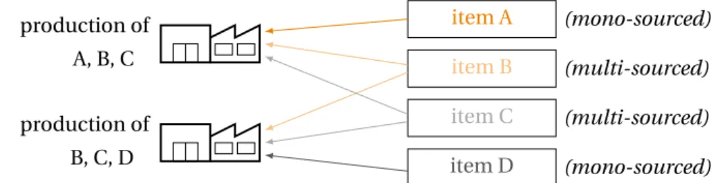
Multi-sourcing of production is a strategic decision in Supply Chain Management (i.e., a long-term decision). It consists in deciding if a plant should have the ability to produce an item. For example, in Figure 1.2, the first plant can produce items A, B and C while the second one can produce items B, C and D. Then, items A and D are said to be mono-sourced since each can

Chapter 1. Introduction L on g ter m S hor t ter m

Strategic Tactical Operational Execution

Capacity-sizing

Multi-sourcing (Part III)

Assignment models

Lot-sizing (Part I)

Continuous-time inventory models

Production planning (Part II)

Discrete-time inventory models

Scheduling

Figure 1.1 – Decision horizon

be produced by only one plant whereas items B and C are said to be multi-sourced since they can be produced by at least two plants. The first characteristic of multi-sourcing decisions is their horizon. They take time to be implemented and have long-term impact on Supply Chain Management. Second, multi-sourcing decisions are taken in a highly uncertain environment. Among others, the future customer demand, the reliability of means of production and the future availability of raw materials are imperfectly known. Finally, multi-sourcing decisions will constrain future production decisions (i.e., mid-term decision). Precisely, they determine the flexibility of the plants and the ability to balance the workload between them.

production of A, B, C production of B, C, D item A (mono-sourced) item B (multi-sourced) item C (multi-sourced) item D (mono-sourced)

Figure 1.2 – Multi-sourcing of production of four items in two plants

Considering its applications, Argon Consulting chooses to model the demand as the main source of uncertainty with a fixed and known total volume of demand. (In its applications, Argon Consulting is interested by the ability to face variations in the product mix and not in the volume of demand.) In Chapter 9, we model the problem as a stochastic program with recourses where first-stage variables are the assignment of items to plants and second-stage variables are the production decisions. In order to deal with randomness and to capture the long-term impact and the risk of assignment decisions, we rely on risk measures, which are tools from financial theory used to quantify the risk of a financial position. We choose to use the Average-Value-at-Risk (A V@R) applied to the inventory level of items. To the best of our knowledge, it is almost the first time that such a tool is used in Supply Chain applications. High inventory level is expensive but enables an easy satisfaction of the demand. Reducing inventory is then risky and Average-Value-at-Risk aims at quantifying the risk of this decision.

The Average-Value-at-Risk atα% (also known as Expected Shortfall or

Conditional-Value-at-Risk) can be interpreted as the expectation restricted to theα% worst cases, i.e., α% lowest

values of inventory. It enables the decision maker to have an indicator that captures both the shortfall probability and the undelivered quantity (which are strongly linked to two indicators 2

1.2. Continuous-time inventory models

used to measure service level: the cycle service level and the fill rate service level). Moreover, the

parameterα provides a simple way to address the control of the risk level and the

Average-Value-at-Risk can be linearized. We apply a classical approximation scheme to solve the stochastic program by doing first a two-stage approximation and then a sampling of scenarios in order to get a mixed integer linear program (MILP), which leads to a tractable formulation.

Real datasets given by Argon Consulting’s clients contain only historical values of production and sales. Since we do not know the actual demand, we propose in Chapter 7 a probabilistic model to generate possible realizations of demand from historical values. This model is based on Dirichlet distributions and aims at being easy to use while being reasonable. Its only input is a forecast demand (which can be the historical sales or the historical forecast) and a volatility which is a percentage standing for the accuracy of the forecast. (The smallest the volatility the most accurate the forecast.) Our probabilistic model provides scenarios of demand such that the total volume of demand is the same in each scenario, such that the expectation of a realization is equal to the forecast and such that the standard deviation divided by the expectation is close to the volatility. This model meets the assumption made by Argon Consulting on the demand, has few parameters and is easy to simulate (even conditionally to the past).

Finally, on real datasets, computation times may be long. Up-to-date solvers are often unable to find a feasible solution of the problem. Then, we propose a heuristic that enables us to quickly find a feasible solution of the multi-sourcing problem. The returned solution can be directly used by Argon Consulting’s clients or as an initial solution of a generic solver.

The experimentations made in Chapter 10 already prove that the company that provides the datasets can reduce its proportion of multi-sourced items (thus reduce its costs) while keeping a good ability to satisfy demand. However, computer performances and real dataset sizes prevent us from dealing with more than a hundred of scenarios. Thus, the method is dependent on the sampling methods and the choice of a representative set of scenarios is critical. We propose a concrete way to reduce this dependence on the sampling methods based on clustering methods (such as K -means).

1.2 Continuous-time inventory models

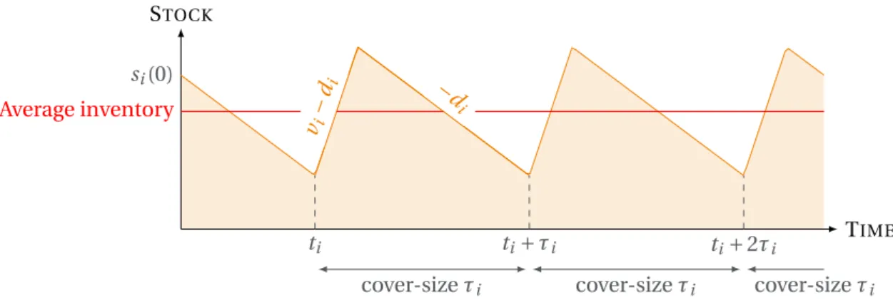
Argon Consulting uses continuous-time inventory models to compute macroscopic parameters at a tactical level (mid-term decisions). Classical examples are the lot-size and the cover-size. The lot-size gives the quantity of a same item produced at each production launch. The cover-size gives the number of time units following a production launch during which inventory must be positive. These parameters are used as input for other decision processes in Supply Chain such as the Material Requirement Planning (MRP). For example, having an estimate of the lot-sizes or the cover-sizes allows to decide the quantity of raw materials that must be ordered. They are also used as input to plan the production since they give the sizes of produced lots. (When studying discrete-time models, we will propose to remove this constraint from the models.) Continuous-time inventory models assume a continuous vision of time. The seminal model

known as the Economic Order Quantity (EOQ) model fromHarris(1913) gives the optimal

Chapter 1. Introduction

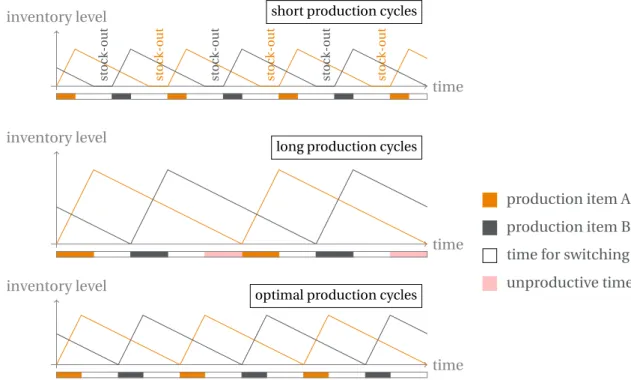
and holding costs are difficult to compare. Argon Consulting aims at finding the optimal lot-sizes (or cover-lot-sizes) from the flexibility of its assembly lines, which is considered as fixed and defined by previous Supply Chain processes. An assembly line can produce several items but loses time when switching from the production of one item to another. Considering a constant demand rate, Figure 1.3 shows the consequences of several lengths of production cycles. Too short production cycles lead to stock-out since too much time is spent switching between the production of two items whereas too long production cycles lead to unnecessary high inventory and unproductive time. In real datasets, assembly lines produce a lot of items and time lost due to switching between different items is modeled by a maximal number of setups.

time inventory level st ock-o ut st o c k-o ut st ock-o ut st o c k-o ut st ock-o ut st ock-o ut time inventory level time inventory level production item A production item B time for switching unproductive time

short production cycles

long production cycles

optimal production cycles

Figure 1.3 – Continuous-time inventory model for a line producing two items

Replacing the ordering costs by an upper bound on the number of setups, we propose in Chapter 3 generalizations of the classical EOQ formula for multiple items. They have already been useful for Argon Consulting. Specifically, we study continuous and integer numbers of setups in deterministic and stochastic settings. Moreover, we also study in Chapter 4 an extension that considers several parallel assembly lines and show that the problem can be stated as a concave minimization problem over a polyhedron (for which it exists an extensive literature).

1.3 Discrete-time inventory models

Discrete-time inventory models (also called dynamic lot-sizing problems) assume that time is decomposed into discrete periods. They are used by companies to plan their short-term production. A classical model is the Capacitated Lot-Sizing Problem (CLSP). It considers an assembly line producing several items during a finite number of periods. The demand for each 4

1.3. Discrete-time inventory models

item is deterministic and given for each period. It aims at minimizing the sum of the holding costs (due to inventory carried from a period to the following) and the setup costs (fixed cost due to launch of the production) subject to the capacity of the assembly line.

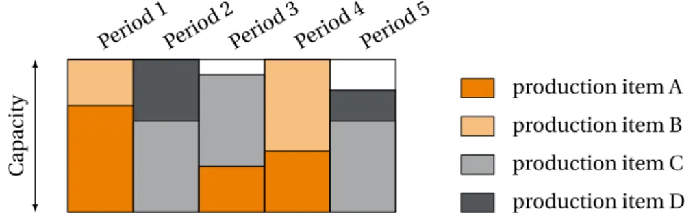
As already mentioned in Section 1.2, the drawback of this formulation according to Argon Consulting and its clients is the difficulty to estimate the value of the setup costs. On the other hand, estimating the maximal number of setups for a period is an easy task for Argon Consulting’s clients. We propose in Chapter 5 a model derived from the Capacitated Lot-Sizing Problem that replaces the setup costs by an upper bound on the number of setups. Figure 1.4 shows an example of production planning of four items when at most two items can be produced during a period. To the best of our knowledge, this model is new and has not been studied in the literature. Period 1 Period 2 Period 3 Period 4 Period 5 C ap acit y production item D production item C production item B production item A

Figure 1.4 – Production planning of four items for five weeks

Our lot-sizing problem can be written as a mixed integer linear program (MILP). We get several theoretical results in the deterministic setting that show the difficulties of the problem. As ex-pected, this problem is NP-hard. A classical method to help solve mixed integer linear programs consists in relaxing some constraints to get a bound on the optimal value of the problem. We show that several natural formulations all yield the same continuous relaxation. Finally, we were left with the following question: what is the complexity status of our lot-sizing problem when there is no capacity constraints and when the maximal number of setups per period is equal to 1? Mathematically, it can be formulated as follows. Consider the problem

min T X t =1 X i ∈I his_ti s. t. s_ti= si_{t −1}+ qti− dti ∀t ∈ [T ], ∀i ∈I, qi_t6M xi_t ∀t ∈ [T ], ∀i ∈I, X i ∈I xti61 ∀t ∈ [T ], xti∈ {0, 1} ∀t ∈ [T ], ∀i ∈I, qit, sit>0 ∀t ∈ [T ], ∀i ∈I, (P)

where M is a big positive number, and for each period t and each item i , the demand d_tiand

the holding cost hiare given nonnegative real numbers, and the inventory si_t, the produced

Chapter 1. Introduction

Open question. What is the complexity status of (P)?

In practice, the demand is not always deterministic. We propose in Chapter 6 a stochastic version of our lot-sizing problem based on Stochastic Programming (see Section 1.1). The difference is that we do not use a risk-averse constraint (A V@R) but stick to the classical risk-neutral vision (the expectation). Indeed, production is a repeated decision and a failure at one period is easy to compensate with another period.

Moreover, in a stochastic setting, we must allow backorder because production resources are limited and it may be impossible to cover every single possible realizations of demand. Here, they come with costs in the objective function. Except when they are enshrined through contracts with the customers, backorder costs can be hard to estimate. We adapt from the literature a method based on the news-vendor problem (one of the oldest stochastic models) to link the backorder cost and the desired portion of satisfied demand.

As in Section 1.1, our stochastic lot-sizing problem is also solved by doing first a two-stage approximation and then a sampling of scenarios in order to get a mixed integer linear program. Since scenarios were not provided by our partner, we generate them using the probabilistic model mentioned in Section 1.1.

The experimentations made in Chapter 7 seem to show that the company that provides the datasets can reduce its inventory costs while keeping a good ability to satisfy the demand. However, as in Section 1.1, computer performances, real dataset sizes and limited time to return a production planning prevent from dealing with more than twenty scenarios. Since the method is dependent on the sampling methods, we propose again a concrete way to reduce this dependence on the sampling methods based on clustering methods (such as K -means).

1.4 Extensions

In Part IV, we present two extensions of our work. The first is an alternative version of the multi-sourcing problem addressed in Part III. The difference is that the company has a limited budget to invest in flexibility. In this case, the company aims at deciding an assignment which maximizes the demand that can be satisfied. We model this alternative problem and show that it is NP-hard in several simple cases.

The second is an extension of the inventory models addressed in Part I and II. We aim at computing the cover-sizes at mid-term horizon using a model relying on production planning at short-term. We model this alternative problem and experimentally show that it has many drawbacks compared to the continuous-time inventory models.

1

Introduction (version française)

La recherche effectuée dans le cadre de cette thèse CIFRE porte sur la gestion de la Supply Chain. Elle a été financée par Argon Consulting, cabinet de conseil indépendant dont la mission est d’aider ses clients à améliorer l’ensemble de leur Supply Chain (de l’approvisionnement en matières premières à la livraison des produits finis) et est menée dans le cadre d’un partenariat industriel avec l’École des Ponts ParisTech. L’objectif est de modéliser et de développer des méthodes pour gérer de manière optimale certaines fonctions spécifiques de la Supply Chain. Le point commun des trois sujets développés dans cette thèse est la flexibilité. Nous définissons la flexibilité comme la capacité à fournir un service ou un produit à un client dans un environ-nement incertain. Selon le niveau de décision, la flexibilité est soit une contrainte (comme la capacité d’une ligne de production à passer facilement de la production d’un article à un autre) soit une variable de décision (comme décider entre spécialisation et polyvalence). En général, décider de la flexibilité d’un système est une décision à long terme (et parfois à moyen terme). Afin d’aider à la compréhension globale des sujets, nous avons choisi d’introduire les trois sujets en commençant par les décisions à long terme, puis les décisions à moyen terme, et enfin les décisions à court terme. Cependant, ce manuscrit suit un ordre différent dû à l’introduction de notions et de résultats réutilisés d’une partie sur l’autre. Les décisions à long terme étudiées dans cette thèse (Partie III) portent sur le multi-sourcing de la production qui vise à décider de la flexibilité des moyens de production tout en gardant un coût raisonnable. Les décisions à moyen terme (Partie I) et les décisions à court terme (Partie II) traitent toutes deux de la réduction des stocks sous la contrainte des décisions de flexibilité déjà prises. Cependant, les décisions à moyen terme qui nous intéressent visent à calculer des indicateurs qui pilotent plusieurs processus de la Supply Chain alors que les décisions à court terme qui nous intéressent visent à décider de la production qui doit être lancée.

Les trois sujets de cette thèse et d’autres exemples sont placés sur la Figure 1.1 en fonction de leur horizon de décision.

1.1 Multi-sourcing de la production

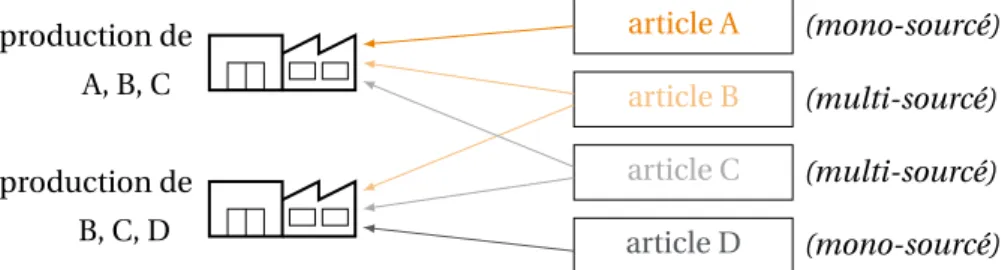
Le multi-sourcing de la production est une décision stratégique dans la gestion de la Supply Chain (i.e. une décision à long terme). Elle consiste à décider si une usine doit avoir la capacité de produire un article. Par exemple, dans la Figure 1.2, la première usine peut produire les

Chapter 1. Introduction (version française) Lo n g ter me C our t ter me

Stratégique Tactique Opérationnel Exécution

Dimensionnement de capacité

Multi-sourcing (Part III)

Modèles d’affectation

Dimensionnement de lot (Part I)

Modèles de stock en temps continu

Plan de production (Part II)

Modèles de stock en temps discret

Ordonnancement

Figure 1.1 – Horizon de décision

articles A, B et C tandis que la seconde peut produire les articles B, C et D. Les articles A et D sont dits mono-sourcés puisque chacun peut être produit par une seule usine alors que les articles B et C sont dits multi-sourcés puisqu’ils peuvent être produits par au moins deux usines. La première caractéristique des décisions de multi-sourcing est leur horizon. Leur mise en œuvre prend du temps et a un impact à long terme sur la gestion de la Supply Chain. Deuxièmement, les décisions de multi-sourcing sont prises dans un environnement très incertain. Entre autres, les demandes futures des clients, la fiabilité des moyens de production ou la disponibilité future des matières premières sont mal connues. Enfin, les décisions de multi-sourcing contraignent les décisions de production futures (décision à moyen terme). Plus précisément, elles déterminent la flexibilité des usines et la capacité à équilibrer la charge de travail entre elles.

production de A, B, C production de B, C, D article A (mono-sourcé) article B (multi-sourcé) article C (multi-sourcé) article D (mono-sourcé)

Figure 1.2 – Multi-sourcing de la production de quatre articles sur deux usines

Considérant ses applications, Argon Consulting choisit de modéliser la demande comme princi-pale source d’incertitude avec un volume total de demande fixe et connu. (Dans ses applications, Argon Consulting s’intéresse à la capacité de faire face aux variations du mix produit et non du volume de la demande.) Dans le Chapitre 9, nous modélisons le problème comme un

pro-gramme stochastique avec recours où les variables de première étape sont l’affectation des

articles aux usines et les variables de deuxième étape sont les décisions de production. Afin d’intégrer le caractère aléatoire et de prendre en compte l’impact à long terme et le risque des décisions d’affectation, nous nous appuyons sur les mesures de risque, qui sont des outils de la théorie financière utilisés pour quantifier le risque lié à une position financière. Nous choisis-sons d’utiliser l’Average-Value-at-Risk (A V@R) appliquée au niveau de stock des articles. À’ notre connaissance, un tel outil a rarement été utilisé dans des applications Supply Chain. Un niveau de stock élevé est coûteux mais permet de satisfaire facilement la demande. La réduction des stocks est alors risquée et l’Average-Value-at-Risk vise à quantifier le risque lié à cette décision.

L’Average-Value-at-Risk àα% (aussi connue sous le nom d’Expected Shortfall ou de

1.2. Modèles de stock en temps continu

Value-at-Risk) peut être interprétée comme l’espérance restreinte auxα% pires cas, i.e. au α%

plus basses valeurs du stocks. Elle permet au décideur de disposer d’un indicateur qui saisit à la fois la probabilité de rupture et la quantité non livrée (qui sont fortement liés à deux indicateurs utilisés pour mesurer le niveau de service : le cycle service level et le fill rate service level). De

plus, le paramètreα fournit un moyen simple de contrôler le niveau de risque et

l’Average-Value-at-Risk peut être linéarisée. Nous appliquons un schéma d’approximation classique pour résoudre le programme stochastique en faisant d’abord une approximation en deux étapes, puis un échantillonnage de scénarios afin d’obtenir un Programme Linéaire en Nombres Entiers

(PLNE) menant à une formulation tractable.

Les jeux de données réelles fournies par les clients d’Argon Consulting ne contiennent que les valeurs historiques de production et de ventes. Comme nous n’avons pas la demande réelle, nous proposons dans le Chapitre 7 un modèle probabiliste pour générer des réalisations possibles de la demande à partir de valeurs historiques. Ce modèle est basé sur les distributions

de Dirichlet et vise à être facile à utiliser tout en gardant une certaine vraisemblance. Sa seule

entrée est une demande prévisionnelle (qui peut être l’historique des ventes ou l’historique des prévisions) et une volatilité qui est un pourcentage représentant l’exactitude de la prévision. (Plus la volatilité est faible, plus la prévision est précise.) Notre modèle probabiliste fournit des scénarios de demande de sorte que le volume total de la demande soit le même dans chaque scénario, de sorte que l’espérance de chaque réalisation soit égale à la prévision et que l’écart type divisé par l’espérance soit proche de la volatilité. Ce modèle répond aux hypothèses faites par Argon Consulting sur la demande, a peu de paramètres et est facile à simuler (même conditionnellement au passé).

Enfin, sur des jeux de données réelles, les temps de calcul peuvent être longs. Les solveurs modernes sont souvent incapables de trouver une solution réalisable au problème. Nous pro-posons une heuristique qui permet de trouver rapidement une solution réalisable au problème du multi-sourcing. La solution retournée peut être utilisée directement par les clients d’Argon Consulting ou comme solution initiale d’un solveur générique.

Les expérimentations faites dans le Chapitre 10 prouvent d’ores et déjà que l’entreprise qui fournit les jeux de données peut réduire sa proportion d’articles multi-sourcés (réduisant ainsi ses coûts) tout en conservant une bonne capacité à satisfaire la demande. Cependant, les performances des ordinateurs et la taille réelle des jeux de données empêchent de traiter plus d’une centaine de scénarios. La méthode dépend donc de l’échantillonnage et le choix d’un ensemble représentatif de scénarios est essentiel. Nous proposons une façon concrète de réduire cette dépendance vis-à-vis de l’échantillonnage basées sur les méthodes de clustering (telles

K -means).

1.2 Modèles de stock en temps continu

Argon Consulting utilise des modèle de stock en temps continu pour calculer des paramètres macroscopiques au niveau tactique (décisions à moyen terme). Les exemples classiques sont la taille de lot et la taille de la couverture. La taille de lot donne la quantité d’un même article produite à chaque lancement de production. La taille de la couverture indique le nombre d’unités de temps suivant un lancement de production pendant lequel le stock doit être positif.

Chapter 1. Introduction (version française)

Ces paramètres sont utilisés comme entrée pour d’autres processus de décision dans la Supply Chain comme pour la planification des besoins en composants (MRP). Par exemple, avoir une estimation des tailles de lot ou des tailles de couverture permet de décider de la quantité de matières premières qui doit être commandée. Ils sont également utilisés comme entrées pour planifier la production puisqu’ils donnent les tailles de lot à produire. (Lors de l’étude des modèles en temps discret, nous proposerons de supprimer cette contrainte des modèles.) Les modèle de stock en temps continu présupposent une vision continue du temps. Le modèle

fondateur connu sous le nom de Formule de Wilson et développé parHarris(1913) permet

de calculer le compromis optimal entre les coûts de commande et les coûts de stockage. En pratique, la formule de Wilson est difficile à utiliser car les coûts de commande et de stockage sont difficiles à comparer. Argon Consulting cherche à trouver les tailles de lot (ou tailles de couverture) optimales à partir de la flexibilité de ses lignes de production, qui est considérée comme fixe et définie par les processus amont de la Supply Chain. Une ligne de production peut produire plusieurs articles mais perd du temps lorsqu’elle change de la production d’un article à un autre. En considérant un taux de demande constant, la Figure 1.3 montre les conséquences de plusieurs longueurs de cycles de production. Des cycles de production trop courts entraînent des ruptures de stock car trop de temps est perdu dans les changements de production, alors que des cycles de production trop longs entraînent des sur-stocks et des temps improductifs. Dans les jeux de données réelles, les lignes de production produisent beaucoup d’articles et le temps perdu dû au changement entre différents éléments est modélisé par un nombre maximal de changements. temps niveau de stock rupt u re rupt u re rupt u re rupt u re rupt u re rupt u re temps niveau de stock temps niveau de stock production article A production article B temps de changement temps improductif

cycles de production courts

cycles de production longs

cycles de production optimaux

Figure 1.3 – Modèle de stock en temps continu pour une ligne produisant deux articles

En remplaçant les coûts de changement par une borne supérieure sur le nombre de change-ments, nous proposons dans le Chapitre 3 des généralisations de la formule classique de Wilson pour des cas avec plusieurs articles. Elles sont désormais utilisées par Argon Consulting. En 10

1.3. Modèles de stock en temps discret

particulier, nous étudions les cas où les tailles de couverture sont continues ou entières dans des contextes déterministes et stochastiques. De plus, nous étudions également dans le Chapitre 4 une extension qui prend en compte plusieurs lignes de production parallèles et montre que le problème peut être décrit comme un problème de minimisation concave sur un polyèdre (pour lequel il existe une vaste littérature).

1.3 Modèles de stock en temps discret

Les modèles de stock en temps discret (également appelés dynamic lot-sizing problem) sup-posent que le temps est décomposé en périodes discrètes. Ils sont utilisés par les entreprises pour planifier leurs productions à court terme. Un modèle classique est le Capacitated Lot-Sizing

Problem (CLSP). Il s’agit d’une ligne de production produisant plusieurs articles pendant un

nombre fini de périodes. La demande pour chaque article est déterministe et donnée pour chaque période. Il vise à minimiser la somme des coûts de stockage (dus aux stocks reportés d’une période à l’autre) et des coûts de lancement (coûts fixes liés au lancement de la production) sous contrainte de capacité de la ligne de production.

Comme déjà mentionné en Section 1.2, l’inconvénient de cette formulation selon Argon Con-sulting et ses clients est la difficulté d’estimer la valeur des coûts de lancement. D’autre part, l’estimation du nombre maximal de lancements pour une période donnée est une tâche facile pour les clients d’Argon Consulting. Nous proposons dans le Chapitre 5 un modèle dérivé du Capacitated Lot-Sizing Problem qui remplace les coûts d’installation par une borne supérieure sur le nombre de lancements. La Figure 1.4 montre un exemple de planification de la production de quatre articles sous contrainte qu’au plus deux éléments peuvent être produits pendant une période. À notre connaissance, ce modèle est nouveau et n’a pas été étudié dans la littérature.

Période 1 Période 2 Période 3 Période 4 Période 5 C ap acit é production article D production article C production article B production article A

Figure 1.4 – Planification de la production de quatre articles sur cinq semaines

Notre problème de taille de lot peut être écrit comme un Programme Linéaire en Nombres

Entiers (PLNE). Nous obtenons plusieurs résultats théoriques dans le cadre déterministe qui

montrent les difficultés du problème. Comme prévu, ce problème est NP-hard. Une méthode classique pour aider à résoudre les programmes linéaires en nombres entiers consiste à relâcher certaines contraintes pour obtenir une borne sur la valeur optimale du problème. Nous mon-trons que plusieurs formulations naturelles produisent toutes la même relaxation continue. Enfin, nous n’avons pas pu répondre à la question suivante : quelle est la complexité de notre problème de Lot-Sizing lorsqu’il n’y a pas de contraintes de capacité et que le nombre maximal de changements par période est égal à 1 ? Mathématiquement, il peut être formulé comme suit.

Chapter 1. Introduction (version française) Considérons le problème min T X t =1 X i ∈I hisi_t s. t. si_t= s_{t −1}i + qit− dti ∀t ∈ [T ], ∀i ∈I, qi_t6M xi_t ∀t ∈ [T ], ∀i ∈I, X i ∈I xi_t61 ∀t ∈ [T ], xi_t∈ {0, 1} ∀t ∈ [T ], ∀i ∈I, qi_t, si_t>0 ∀t ∈ [T ], ∀i ∈I, (P)

où M est un grand réel positif et pour chaque période t et chaque article i , la demande d_ti et

le coût de stockage hisont des nombres réels positifs et le stock si_t, la quantité produite qi_t et

l’indicateur de lancement xi_tsont les variables de décision.

Question ouverte. Quelle est la complexité de (P) ?

En pratique, la demande n’est pas toujours déterministe. Nous proposons dans le Chapitre 6 une version stochastique de notre problème de taille de lot basée sur la programmation stochastique. (voir Section 1.1). La différence est que nous n’utilisons pas une contrainte d’aversion au risque (A V@R) mais nous nous en tenons à la vision classique de neutralité au risque (l’espérance). En effet, la production est une décision répétée et un échec lors d’une période est facile à compenser par une autre période.

De plus, dans un contexte stochastique, nous devons autoriser le backorder (i.e. les commandes livrées en retard) parce que les capacités de production sont limitées et qu’il peut être impossible de couvrir toutes les réalisations possibles de la demande. Ici, le backorder vient avec des coûts dans la fonction d’objectif. À moins qu’ils ne soient contractualisés avec les clients, les coûts de backorder peuvent être difficiles à estimer. Nous adaptons une méthode de la littérature basée sur le problème du vendeur de journaux (l’un des plus anciens modèles stochastiques) pour lier le coût de backorder et le niveau souhaité de la demande satisfaite.

Comme dans la Section 1.1, notre problème de taille de lot stochastique est également résolu en faisant d’abord une approximation en deux étapes, puis un échantillonnage de scénarios afin d’obtenir un programme linéaire en nombres entiers. Comme les scénarios de demande n’ont pas été fourni par notre partenaire, nous les générons en utilisant le modèle probabiliste mentionné en Section 1.1.

Les expérimentations faites dans le Chapitre 7 tendent à montrer que l’entreprise qui fournit les jeux de données peut réduire ses coûts de stockage tout en conservant une bonne capacité à satisfaire la demande. Cependant, comme dans la Section 1.1, les performance des ordinateurs, la taille réelle des jeux de données et le temps limité pour retourner un plan de production empêchent de traiter plus de vingt scénarios. Puisque la méthode dépend de l’échantillonnage, nous proposons encore une fois une façon concrète de réduire cette dépendance, fondée sur les méthodes de clustering (comme K -means).

1.4. Extensions

1.4 Extensions

Dans la Partie IV, nous présentons deux extensions de notre travail. La première est une version alternative du problème de multi-sourcing abordé dans la Partie III. La différence est que l’entreprise a un budget limité à investir dans la flexibilité. Dans ce cas, l’entreprise cherche à décider d’une affectation qui maximise la demande qui peut être satisfaite. Nous modélisons ce problème alternatif et montrons qu’il est NP-difficile dans plusieurs cas simples.

La seconde est une extension des modèles de stock abordés dans la Partie I et II. Notre objectif est de calculer les tailles de couverture à moyen terme à l’aide d’un modèle s’appuyant sur la planification de la production à court terme. Nous modélisons ce problème alternatif et mon-trons expérimentalement qu’il présente de nombreux inconvénients par rapport aux modèles de stock en temps continu.

2

Business context

A Supply Chain is a system of organizations, people, activities, information, and resources in-volved in producing, transforming or moving a product or a service from suppliers to customers. It can be considered for a subsidiary, a whole company or for multiple companies working together. Its activities extend from the procurement of raw materials to their transformation into finished products and their delivery to the costumer.

Supply Chain can fulfill several functions. Most common are procurement, production, distri-bution, storage, shipping, sales and billing, and customer relationship. The work of this thesis deals with production and storage optimization within companies.

2.1 Supply Chain objectives

Supply Chain management consists in finding the right balance between conflicting objectives. They can be classified into three categories: costs, stocks and service.

Costs are the expenses paid by companies as a part of their activities. It can be fixed or variable and direct or indirect. Fixed costs, like rent, insurance and investment costs (such as buying ma-chines), do not depend on the volume of the business activity. On the other hand, variable costs, like shipping or energy costs, directly increase with the volume of the business activity. Direct costs concern resources entirely dedicated to the product manufacturing like procurement of raw materials or worker salaries. Indirect costs support functions that are not directly involved in production like marketing or administration.

Stocks, also called inventory, induce costs for storage space, insurance, broken or stolen goods, and work time to keep registered stock accurate. The main characteristic of inventory is that it is locked-in money until it is transformed (for raw materials) or sold (for finished products). Thus, it prevents from investing this capital in developments like R&D or geographic expansion. Stocks are more comparable to working capital and because of this specificity, they must form their own category in optimization process.

Service or service level measures the ability of the Supply Chain to deliver the right product to the customer while respecting the deadlines. There are many indicators to measure the service level but we can identify two main ones: the cycle service level and the fill rate service level. Both rely on stock-out (i.e., the unavailability of a product at a given time) and on the replenishment cycle which is the time between two consecutive replenishments of the stock. The cycle service

Chapter 2. Business context

level is the probability of not hitting a stock-out during the next replenishment cycle, and thus, also the probability of not losing sales. The fill rate service level represents the fraction of the demand that is delivered without delays or lost sales. The choice of the indicator depends on the industry. Indeed, in the case of complex products like in aeronautics, if one component is missing in the command, it can delay the whole project. Thus delivering the whole command is more important and this makes the cycle service level more relevant. In case of simple products like in mass distribution, it is more relevant to measure the part of demand delivered at due date and this makes the fill rate service level more relevant.

Automotive and luxury industries are good examples of these conflicting objectives. In auto-motive industry, high stock is impossible because of depreciation and diversity of products. However, the service level must be high due to high competition. In luxury industry, availability of the right product in the right store is more critical than production costs but high stocks are still impossible.

In general, industrial agility, which is the ability to face variations in customers’ demand is an efficient way to be competitive if two conditions are satisfied. First, the cost of agility should stay reasonable and second, agility should not be achieved thanks to high stocks. For a company, defining its agility is therefore finding a balance between cost, stock and service.

Industrial agility can be split in two parts: capacitative reactivity and flexibility. Capacitative reactivity is the ability to face variations of the global volume, by being able to produce more products than the estimated demand for example. This concerns over-capacitated industries or industries being able to outsource part of the production. Capacitative reactivity is more critical in sector like process industry since adding overcapacity is extremely expensive and outsourcing can be extremely hard. Flexibility is the ability to face variations of the product mix. Multi-sourcing the production, which means giving to several plants the ability to produce the same product, enables more flexibility but decreases productivity. Increasing stocks would be another way to increase flexibility. Among other, flexibility enables to adapt to an unexpected cannibalization of a product by another. Luxury industry and mass distribution are probably the sectors where being flexible is the most critical due to the vast number of products.

The exact definition of the agility depends on the industrial context but also on the decision level: strategic (long-term), tactical (mid-term) or operational (short-term). At the strategic level, the executive committee has expressed the desired agility and wants to decide an investment in production capacities. Thus, agility is a constraint, cost is an objective to minimize and stock is not really considered. Just between strategic and tactical levels, capacitative reactivity cannot be changed, S&OP (Sales and Operations Planning) process has expressed a desired service level and wants to decide multi-sourcing. Thus, service level is a constraint and cost is an objective. At the tactical and operational levels, service level is an input for the production planning and stock and production are the lever. Thus, service level is a constraint, stock is an objective to minimize and production are the decisions. At very short term horizon, e.g., for scheduling decisions, last-minute optimizations can still be made in order to reach the service level objectives. 16

2.2. Supply Chain organizations

2.2 Supply Chain organizations

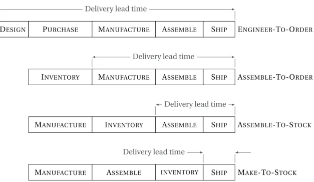
Supply Chain organizations can be classified into four main models described byArnold et al.

(2007) (among others). They are represented in Figure 2.1.

• Engineer-To-Order (ETO). The customer is involved in the design and gives engineering requirements and specifications which enables a lot of customization and a specific design. Due to purchasing of raw materials and to designing, the consequences are long delivery lead times. Classical domains are aeronautic or aerospace industries.

• Make-To-Order (MTO). Products are made from standard components but with

custom-designed components. Therefore, inventory are only composed of raw materials and delivery lead time are still long. For example, marine energy turbines can be produced with a MTO organization.

• Assemble-To-Order (ATO). Customer involvement is limited to selection of component

options. Thus, inventory is only composed of semi-finished products ready for assembly components and delivery lead time are short. Production of laptops partially follows this organization.

• Make-To-Stock (MTS). Customer has very little involvement in the design. Products are en-gineered and manufactured to fill stocks which supply clients demand. This organization enables the shortest delivery lead time. The majority of mass distribution products uses this organization.

For some products, the best organization is obvious due to size of series. For example, a French aeronautic company produces engines of an aircraft carrier with an ETO organization, but turboshafts of choppers with MTO organization. For other industries, identifying the best organization also depends on the commercial strategy (laptops may also be produced with MTS organization) and it is critical to define which decisions are short-term, mid-term or long-term and to know when costs, stock and service can be impacted.

2.3 Presentation of Argon Consulting

Argon Consulting is an international, independent consulting firm whose mission is to help its clients achieve sustainable competitive advantages through operational excellence. It began its consultancy activity in 2001 and employs over 230 consultants in six offices: Paris, London, Atlanta, Singapore, Melbourne and Mumbai.

Argon Consulting has supported many companies in operational transformation projects (R&D, Procurement, Manufacturing, Supply Chain, Distribution, Services, SG&A, Performance Man-agement, Change Management). Industries served cover Aerospace & Defense (Latécoère, Safran, Thales) and Discrete Manufacturing (Alstom, SNCF, DCNS) which have small-series and large program logic as well as Retail (ADEO, Carrefour, Cdiscount) which sells products or services to large number of customers through multiple channels of distribution. In the mid of these extremes, we also find Automotive (Michelin, PSA, Valeo) where innovation performance and diversity of products are challenging, Consumer Packaged Goods (Bel, Danone, L’Oréal) where decreasing consumption and fluctuation of production costs reduce profitability, and Textile (Galeries Lafayette, Camaïeu, Kiabi) where fast product renewal and fast evolution of sourcing are critical at an operational level. Among other sectors with specific rules, Luxury Goods has a

Chapter 2. Business context

DESIGN PURCHASE MANUFACTURE ASSEMBLE SHIP ENGINEER-TO-ORDER Delivery lead time

INVENTORY MANUFACTURE ASSEMBLE SHIP ASSEMBLE-TO-ORDER Delivery lead time

MANUFACTURE INVENTORY ASSEMBLE SHIP ASSEMBLE-TO-STOCK Delivery lead time

MANUFACTURE ASSEMBLE INVENTORY SHIP MAKE-TO-STOCK Delivery lead time

Figure 2.1 – Supply Chain organizations and lead times (fromArnold et al.(2007))

highly erratic demand and is extremely competitive, Pharmaceutical Industry (Merck, Sanofi, Servier) has an economic pressure applied by state authorities due to imbalance of the health insurance systems and Energy & Utilities (EDF, ENGIE) is capital-intensive, highly cyclical, fully globalized and at the heart of geostrategic issues.

Argon Consulting began as a consultancy company specialized in logistic. Growing, it acquired expertise in every level of the Supply Chain. Argon Consulting describes itself as a multi-specialized firm whose competitive advantage comes from its ability to quantify their studies. Through this thesis, the objective is to find an unified framework for some recurrent problems. Moreover, Argon Consulting wants to test scientifically the accuracy and the efficiency of the developed models.

2.4 Argon Consulting’s clients cases

Argon Consulting’s clients cases considered in this thesis fall into Assemble-To-Order and Make-To-Stock organizations. We study two cases in this thesis. The first case is both tactical and operational. It occurs when flexibility of means of production is already defined and we aim at deciding which stocks and production levels would enable the company to achieve the desired service level. The second case is more strategic. It occurs when capacity reactivity is already defined and we aims at deciding the multi-sourcing of production which will ensure enough flexibility at tactical and operational levels.

2.4.1 Production planning

Production planning is part of the production function of the Supply Chain and occurs at tactical and operational levels when the flexibility of means of production is already defined. In 18

2.4. Argon Consulting’s clients cases

Assemble-To-Order and Make-To-Stock organizations, stocks are the last levers on flexibility and there must be enough of them to serve the demand at due dates. Then, production planning problem consists in deciding the orders of production, i.e., when production starts and how much is produced, which defines stocks and allows to achieve the desired service level.

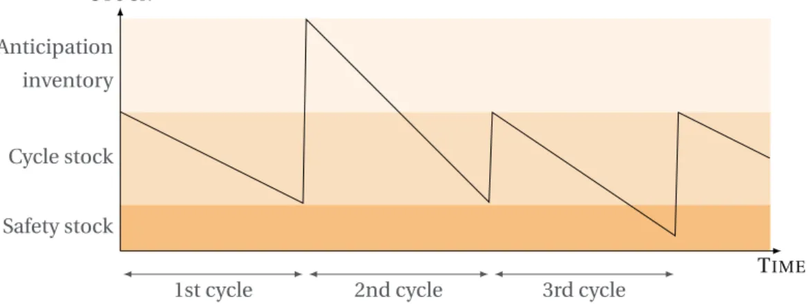
Difficulties of this problem come from the many constraints that prevent last minute production. First, production capacities are limited. Thus, production must be anticipated in order to deliver during peak selling season, promotion program, vacation shutdown, etc. It leads to inventory called anticipation inventory. Second, demand and lead time have random variations. If demand or lead time are greater than forecast, a stock-out can occur. To prevent it, safety stocks are kept as a reserve. Finally, since the flexibility of the means of production is limited, lot-size inventories also called cycle stocks are needed. They form the portion of stocks that varies over time due to production and demand fulfillment. The different parts of the inventory are represented in Figure 2.2. Safety stock Cycle stock Anticipation inventory TIME STOCK

1st cycle 2nd cycle 3rd cycle

In the first cycle, cycle stock enables the company to satisfy perfectly the demand. In the second cycle, an increase in the demand is announced. So, an anticipation inventory is produced in addition to the cycle stock. In the third cycle, the demand is bigger than expected. Thus part of the demand is satisfied using the safety stock.

Figure 2.2 – Inventory decomposition

Production planning aims at minimizing cumulative stocks subject to constraints defined at a higher level.

Service level is the first constraint. In our case, Argon Consulting’s clients want to reach a desired service level which depends on the strategy of the company. It is a trade-off between several objectives as loss of reputation, intended costs, risk, benefits, etc. Production planning problems take it as an input since service level is a long-term decision whereas production decisions are mid-term decisions. Since we are interested in Assemble-To-Order and Make-To-Stock models, we will consider mainly the fill rate service level as defined in Section 2.1.

Most of industrial costs are already fixed. In our case, they are modeled by the capacity and the flexibility. Indeed, capacities of plants or assembly lines and their flexibility are strategic decisions whereas production decisions are tactical or operational decisions. Thus, when production planning problems occur, they cannot be changed. Capacity constraints are easy to