Science Arts & Métiers (SAM)
is an open access repository that collects the work of Arts et Métiers Institute of Technology researchers and makes it freely available over the web where possible.
This is an author-deposited version published in: https://sam.ensam.eu Handle ID: .http://hdl.handle.net/10985/6756
To cite this version :
Abir ISSA, Annie-Claude BAYEUL-LAINE, Gérard BOIS - Numerical Simulation of Flow Field Formed in Water Pump-Sump - In: IAHR - 24th Symposium on Hydraulic Machinery and Systems, Argentina, 2008-10 - IAHR 24th Symposium on Hydraulic Machinery and Systems - 2008
IAHR
24th Symposium on Hydraulic Machinery and Systems OCTOBER 27-31,FOZ DO IGUASSU
RESERVED TO IAHR
NUMERICAL SIMULATION OF FLOW FIELD FORMED IN
WATER-PUMP SUMP
Issa Abir. Bayeul Annie- Claude. Bois Gerard LML-ENSAM
8,bd LouisXII 59000 Lille
ISSA@etudiants.ensam.eu annie-claude.bayeul@ensam.eu Gerard.Bois@ensam.eu
ABSTRACT
Two fundamental types of flow problems besetting water intakes are swirling flow problems in the pump sump and sediment problems at entrance or within intakes. Both problems reduce intake performance and lead to increased plant operating costs.
Experiments were conducted in a laboratory** in order to select best positions of the suction pipe of a water-intake sump. These experiments show qualitative results concerning flow disturbances in the pump-intake related to sump geometries and position of the pump intake. The purpose of the paper is to reproduce the flow pattern and confirm the geometrical parameter influences of the flow behavior in such a pump.
The numerical model solves the Reynolds averaged Navier-Stokes (RANS) equations with a near- wall turbulence model. In the validation of this numerical model, emphasis was placed on the prediction of the number, location, size and strength of the various types of vortices.
The paper mainly focuses first, on mesh geometry turbulence model, closures and boundary conditions. Secondly, a comparison of different flow patterns for several intake locations in the sump will be presented.
KEY WORD: Pump sump-Open channel flow- Free surface vortices-submerged vortices-air entraining- CFD-Turbulent model- Numerical simulation-
INTRODUCTION
Several types of plants use hydraulic pumps to withdraw water from a reservoir or a river. Water pumps intakes generally leads to a vertical tube placed in a sump which geometrical characteristics are generally imposed by the immediate pump environment, with geometrical constrains, resulting in a poor design of the intake or in a channel surroundings or finally insufficient pump intake submerge depth.
These geometrical constrains may cause strong non uniformities inside the sump and at pump intake sections. Low intake submerge depth could also result in the formation of the air entraining free surface vortices that could as well promote cavitation.
Non uniform inlet flow field at sump entrance even far from pump intake section can also leads to accumulative effects due to 3D boundary layers development on the side-wall creating corners vortices that can be strength by local strong streamline curvature when approaching pump intake.
All these non uniformities cause flow instabilities, vibration and other undesirable phenomena that can cause operating difficulties and frequent maintenance of the whole pump arrangements.
Experimental investigations have already been made for example in the Iowa institute of hydraulic research (Nakano1988, 1989, 1990, 1991; Ettema and Nakato1990) to reduce non uniformities of specific flow and geometrical conditions. More basic studies have been also conducted to establish empirical criteria for vortex formation and avoidance, (for example Anwar1966; Anwar and Amphlett1980; Daggett and Keulegan1972).
The use of numerical approach starts with Tagomori and Gotoh (1989) in order to study the effects of non uniform inlet flow on vortex generation and the effects of additional devices to prevent vertical flow formation. They have used a finite volume method to solve the RANS equations with the k-ε model. Takata et al (1992) report large eddy simulations of pump intake flows at low Reynolds number (104). More recently, CFD benchmarks have been performed by Matsui et al. (2006) in order to compare different software results with experiments.
Constantinescu and Patel (1998) have developed a CFD model to solve RANS equations and two turbulence model equations. Their case study was selected according to a commonly used design criteria and also corresponds to experimental configurations previously studied in the laboratory** of the first author of this paper. This is the reason why the geometrical configuration proposed in this last paper has been chosen for the present work in order to study the influence of submergence and inlet boundary layer thickness on flow pattern in a particular sump and intake tube of the pump.
INFLUENCE PARAMETERS ON FLOW PATTERN
Most of flow uniformities caused by what have been developed in the introduction, lead to different kind of vortices that have been generally observed in previous studies.
parts of the vortices are usually formed on the free surface and may transform on air entraining vorticies. Others are formed on side walls and on the floor.
As reported by Constaintinescu and Patel (1998) “the strength of vortices increases with increase of vorticity in the approach flow; the intensity of the free surface and floor-attached vortices increases with asymmetry in the approach flow in the horizontal plane; the intensity of the side-wall attached vortices grows with asymmetry in the approach flow in the vertical plane; back-wall and corner vortices are due to secondary flows; the intensity of floor-attached vortices decreases while that of side-wall and back-wall vortices increases as the floor clearance is increased”. There is a general agreement among the various studies that free-surface vortices are observed as the submergence decreases and air-entraining vortices appear at low submergence. This last aspect has been recently studied and report by Shula and Kshirsagar (2008).
It is also generally assume that the surface tension effects could be neglected owing to the successive studies done by Jain et al (1978), Anwar (1966), Anwar and Amphlett (1980), Padmanabhan and hecker (1984), and Odgaard (1986).
Flow resulting structure inside the sump and in the pump intake generally depends on the following geometrical parameters as shown in figure 1.
Fig. 1 : geometrical parameters Table 1:tests cases and geometrical dimensions Other parametres must be added concerning flow characteries. They are:
¾ Tube Reynolds number, Re=VD/υ
¾ The Froude number related to submergence=U/√gS.
D=0.1m Constant parameters x1=0.9D x2=6.5D l1=l2=1.3D Cases S C H Fr a1 2.25D 0.5D 2.75D 0.023 b1 2D 0.75D 2.75D 0.025 c1 0.75D 2D 2.75D 0.04 d1 0.75D 0.85D 1.6D 0.064 b2 2D 0.75D 2.75D 0.025
¾ The Weber number, we=V2ρD/σ.
This leads to numerous parameters that all influence the flow.
Constantinescu and Patel (1998) point out that it is important to understand clearly the flow pattern using well established numerical methods and good experiments. They have developed a CFD model to solve RANS equations and two turbulence model equations. Their case study was selected, according to commonly used design criteria and also corresponds to experimental configurations previously studied in the laboratory** of the first author of this paper.
This is reason why the geometrical configuration proposed in this last paper has been chosen for the present work. The corresponding velocity profile is a contribution to the knowledge of the flow pattern using a commercial code FLUENT. Specific attention was given to study submergence effects and initial flow conditions at sump entrance as suggested in Constantinescu and Patel conclusions. The chosen geometry is a symmetric one (see fig.1) as well as the inlet flow conditions. Two different boundary layers thicknesses have been applied as inlet flow conditions named respectively as 1 and 2. The corresponding velocity profiles are shown in fig. 2. For some test cases, both k-ε, and k-ω turbulence model were used. This will be discussed further in the paper.
SUMP GEOMETRY TEST CASES
The geometric characterics of the sump are shown in figure1.It has to noted that the intake pipe is placed in the middle of sump (l1=l2=1.3D), at a fixed value of x1(x1=0.9D) from the back wall.
Only the submergence S is variable, for cases a, b, and c. For case d1 the submergence is equivalent
to case c but with a different water level (H). All informations about geometry parameters are represented in table1.
Index 1, 2, present two different boundary layers thicknesses applied as inlet plane flow conditions (see table 1); in case 1, boundary layer is thin; in case 2, boundary layer is thick. The velocity profiles at inlet plane sump (l=7.4D) are given on fig. 2.
Case-1-1 Case-2-1 Case-2-2 Fig. 2: velocity profiles at the entrance of sump. Case1: for boundary layer thin (y=0).
GRID, CALCULATIONS AND BOUNDARY CONDIONS
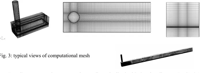
The calculation domain is divided into 3 blocks, as illustrate in figure3. The first block presents the part of sump which is below the tube intake; the second one is the rest of sump which includes the submergence tube intake, assuming an infinity thin tube wall, last one contains the upper part of tube up to the free surface. The resulting computational grid is a structured hexahedral grid with 592050 cells, for cases a1, b1, c1, and 390770 cells for case d1. In order to archive boundary layer
thick, a four block grid far enough was added at the entrance of the sump, as shown in figure3.
Fig. 3: typical views of computational mesh
For all tests cases, the geometry is non-dimensionlized with the pipe diameter D, (D=0.1m). The mean velocity in the pipe is fixed at V=0.286m/s. For all cases, Reynolds, and Weber numbers are respectively: Re=28600, we=115. The values of Froude number are noted in table 1. K-ε turbulence model has been used for all first calculations for all tests cases, but for the cases d1, and b2, k-ω turbulence model has been used in order to test the role of the turbulence model of flow pattern in sump pump, the formation of vortices and their strength.
Concerning boundary conditions, the free surface is a symmetrical condition. Hydrostatic pressure is assumed constant in the entrance plane, and the velocity is imposed in the outlet plane of the tube..
NUMERICAL RESULTS
One way to get qualitative insight views of the flow pattern is to plot what is generally called “particle path”. We can see the particle paths come from either free surface, side walls and/or floor. Among all the test cases, only a few of them are presented here for comparisons because it was impossible to show all tested configurations. Vorticity distributions are also shown generally in some particular planes in order to quantify the different configuration levels.
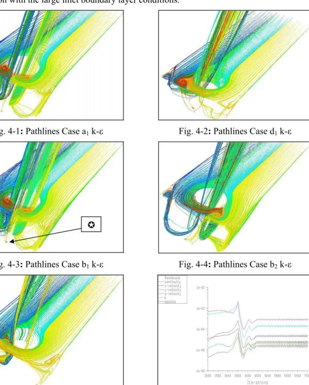
Figures [(4-1) - (4-5)] present the particle path for test cases-1 with the k-ε turbulence model. They show that only the first two test cases give symmetrical results (a1 and b1). Noting that test
c1 and d1 correspond to the smaller submergence cases and b2, corresponding to case b
configuration with the large inlet boundary layer conditions.
Fig. 4-1: Pathlines Case a1 k-ε Fig. 4-2: Pathlines Case d1 k-ε
Fig. 4-3: Pathlines Case b1 k-ε Fig. 4-4: Pathlines Case b2 k-ε
Fig. 4-5: Pathlines Case c1 k-ε Fig. 4-6: convergence history Case c1 k-ε
However, the next figures [(5-1)-(5-3)] corresponding to the same calculation with the k-ω turbulence model, show symmetric results for test cases d1 and b2. All these results can be only
obtained using the free surface as a symmetry plane condition for the calculations. For any other type of boundary conditions, vortices cannot be captured by the calculation method.
From these results, it could be noticed that for low submergences and low values of water level in the sump, flow pattern numerical results using k-ε model may be wrong. In fact, the convergence history gives a good idea of no stable result an example that may occur in such application (fig 4-6).
In case of strong vortices generation, both due to small submergences and thick inlet boundary layers, it is better to use k-ω model. The resulting convergence history, that can be assumed to be the correct one, is shown in figure 5-3.
Fig. 5-1: Pathlines Case b2 k-ω Fig 5-2: Pathlines Case d1 k-ω
Fig. 5-3: convergence Case b2 k-ε
All cases however, show free-surface vortices that can be combined with other vortices coming from side walls. An example of it can be seen in fig. 4-3 and fig 6-1 for some vortices that are created on thebackwall, and another one coming from the side wall (see fig. 6-2).
Fig. 6-1: Pathlines Case b1 k-ε Fig. 6-2: Pathlines Case b1 k-ε
The whole flow structure is rather complicate, but it can be seen, using several view planes that the main two vortices which are on the free surface on both sides of the pump inlet tube goes down to the inlet tube and it seems to vanish inside the tube boundary layers due to the strong curvature and acceleration effects in between the free surface plane and the intake tube section. Corner
vortices also exist due to side wall boundary layers and corner interactions. These vortices can be called as secondary flow pattern and the associated streamlines seems to be captured by the main flow inside the pump intake tube.
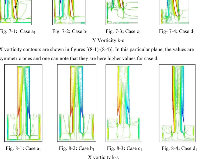
Concerning quantitative aspects, vorticity distributions, they are shown for the same test cases, on the free surface plane and in the vertical mid-plane (corresponding to y=0) and the plane perpendicular to the previous one (corresponding to x=0) using appropriate same scales [(-15)-(+15)] s-1 for comparisons [figs (7-1)-(7-4)]. Both planes also give information inside the vertical intake tube. Looking at cases a and b, the more the submergence decreases, the more the vorticity level is greater (note that the white parts* in the intake tube corresponds to higher value of vorticity (±15 s-1). Lower values appear in case c with non symmetries. Main flow goes to the left part of the tube for cases c and d corresponding to low submergences.
Fig. 7-1: Case a1 Fig. 7-2: Case b1 Fig. 7-3: Case c1 Fig- 7-4: Case d1
Y Vorticity k-ε
X vorticity contours are shown in figures [(8-1)-(8-4)]. In this particular plane, the values are symmetric ones and one can note that they are here higher values for case d.
Fig. 8-1: Case a1 Fig. 8-2: Case b1 Fig. 8-3: Case c1 Fig. 8-4: Case d1
X vorticity k-ε *
CONCLUSIONS
Steady state RANS calculations have been performed on a given geometry already studied in open literature.
Specific attention has been pointed on the effects of submergence and inlet boundary layers for both symmetric sump geometry and inlet flow conditions. Sump grid configuration was also in a pure symmetrical way.
The complex flow pattern that has been already observed experimental can be captured by the numerical method used. However, depending on the turbulence model closure used, one can get non symmetrical results. The k-ω model seems to be the most appropriate one to be able to fit the real flow field if it is assumed that it has to be symmetric.
However it is well known that non symmetrical flow can be obtained with symmetric geometries, using non structured grid for example, or with a week asymmetry on the horizontal plane in flow inlet conditions, or for unsteady calculations. This could be the next step of the present work in order to evaluate the numerical results that are very often observed in real experimental cases.
BIBLIOGRAPHICAL REFERENCES
[1] ANWAR, H. O. (1966). Formation of a weak vortex. Journal of Hydraulic Engineering. Res 4(1), 1-16.
[2] ANWAR.H. O and AMPHLETT, M. B, (1980). Vortices at vertically inverted intake. Journal of Hydraulic Engineering. Res, 18 (2), 123-134.
[3] CONSTANTINEASCU,G, and PATEL, V. C. (1998). Numerical model for simulation of
pump-intake flow and vortices. Journal of Hydraulic Engineering. Div, ASCE, Vol 124, 123-134.Iowa Inst
of Hydr Res. The Univ of Iowa, Iowa City, Iowa
[4] DAGGETT, L. L, and KEULEGAN, G. H. (1972).Similitude conditions in free surface vortex
formulation. Journal of Hydraulic Engineering. Div, ASCE, 100(11), 1565-1580.
[5] ETTEMA, R, NAKATO, T. (1990). Hydraulic model studies of the circulating-water and
essential-service water pump-intake structures. Korea Electric Power Corporation Yonggwang
Station, Units3 and 4. IIHR Limited Distribution Rep. No 173. Iowa Inst of Hydr Res. The Univ of Iowa, Iowa City, Iowa
[6] JAIN, A, K, RAJU, K, G, R, and Grade, R. J. (1978). Vortex formation at vertical pipe intakes. Journal of Hydraulic Engineering. Div, ASCE, 104(10), 1429-1445.
[7] MATSUI, J, KAMEMOTO. K and OKAMURA. T. (2006). CFD benchmark and a model
[8] NAKATO, T. (1988). Hydraulic-laboratory model studies of the circulating-water pump-intake
structure. Florida Power Corporation, Crystal River Units 4and 5. IIHR Rep. No 320, Iowa Inst of
Hydr Res. The Univ of Iowa, Iowa City, Iowa
[9] NAKATO, T. (1989). A hydraulic model study of the circulating-water pump-intake structure. Laguna Verde Nuclear Power station, Unit 1, Commission Federal De Electricidad. IIHR Rep, No 330, Iowa Inst of Hydr Res. The Univ of Iowa, Iowa City, Iowa
[10] NAKATO, T. (1990). A hydraulic model study of the proposed pump-intake and discharge
flume. Florida Power Corporation’s, Crystal River Cooling-Tower Project. IIHR Rep. No 339, Iowa
Inst of Hydr Res. The Univ of Iowa, Iowa City, Iowa
[11] NAKATO, T. (1991). Improvement of pump-approach flows. A hydraulic model study of Union Electric’s Meramec plane circulating-water pump intakes. IIHR Rep. No 348, Iowa Inst of Hydro Res. The Univ of Iowa, Iowa City, Iowa
[12] ODGAAD, J. A. (1986). Free surface air core vortex. Journal of Hydraulic Engineering, ASCE, 112(7), 610-620.
[13] PADMANABHAN, M, and HECKER, G. E. (1984). Scale effects in pump sump models. Journal of Hydraulic Engineering, ASCE, 110(11), 1540-1556.
[14] SHUKLA, S, and KSHIRSAGAR, J.T. (2008). Numerical prediction of a air entrainment in
pump intakes. Corporate Research and Engineering Division. Kirloskar Brothers Limited, Pune,
India.
[15] TAGOMORI, M, and GOTOCH, M. (1989). Flow patterns and vortices in pump-sumps. Proc, Int Symp on Large Hydr Machinery, China press, Beijing. China, 13-22.
[16] TAKATA, I, KAWATA, Y, KOBAYASHI, T, and MORINISHI, Y. (1992) Large eddy
simulation of unsteady turbulent swirl flow in a pump intake. Proc Inst Computational Fluid Dyn.
Elsevier Applied Science, New York, 255-261.
SYMBOLS USED
a1= model test of sump-pump with S=2.25D, C=0.5D, and boundary layer thin
b1= model test of sump-pump with S=2D, C=0.75D, and boundary layer thin
b2= model test of sump-pump with S=2D, C=0.75D, and boundary layer thick.
c1= model test of sump-pump with S=0.75D, C=2D, and boundary layer thin
C= clearance distance from floor
d1= model test of sump-pump with S=0.75D, C=0.85D, and boundary layer thin
D= tube diameter
Fr= Froude number with submergence depth S as length scale. g= acceleration due to gravity.
H= water level in the sump-pump. k= turbulent kinetic energy.
l1, l2= distance from center of pipe to the two side wall.
l= the sump-pump width L= the sump-pump length.
Re= Reynolds number with tube diameter as length scale. S= submergence depth.
U= mean velocity in approach channel. V= mean velocity in the tube.
We= Weber number
x1= clearance from back wall to the axe of tube.
x2= clearance from the entrance of the sump-pump to the axe of tube.
x= Cartesian coordinate. y= normal distance from wall z= vertical distance from floor; ε= rate of turbulent energy dissipation υ= kinematic viscosity
ω= the ratio of ε to k ρ= water density
σ= coefficient of surface tension.