Analyse statistique de données fonctionnelles à
structures complexes
par
ADJOGOU ADJOBO FOLLY DZIGBODI
Département de mathématiques et de statistiqueFaculté des arts et des sciences
Thèse présentée à la Faculté des études supérieures en vue de l’obtention du grade de
Philosophiæ Doctor (Ph.D.) en Statistique
01 Mai 2017
c
Faculté des études supérieures Cette thèse intitulée
Analyse statistique de données fonctionnelles à
structures complexes
présentée par
ADJOGOU ADJOBO FOLLY DZIGBODI
a été évaluée par un jury composé des personnes suivantes :Pierre Duchesne (président-rapporteur) Alejandro Murua (directeur de recherche) Mylène Bédard (membre du jury)
Abbas Khalili (Université McGill) (examinateur externe)
Benoît Perron
(représentant du doyen de la FAS)
Thèse acceptée le 29 Septembre 2017
RÉSUMÉ
Les études longitudinales jouent un rôle prépondérant dans des domaines de recherche va-riés et leur importance ne cesse de prendre de l’ampleur. Les méthodes d’analyse qui leur sont associées sont devenues des outils privilégiés pour l’analyse de l’étude temporelle d’un phénomène donné. On parle de données longitudinales lorsqu’une ou plusieurs variables sont mesurées de manière répétée à plusieurs moments dans le temps sur un ensemble d’in-dividus. Un élément central de ce type de données est que les observations prises sur un même individu ont tendance à être corrélées. Cette caractéristique fondamentale distingue les données longitudinales d’autres types de données en statistique et suscite des méthodo-logies d’analyse spécifiques. Ce domaine d’analyse a connu une expansion considérable dans les quarante dernières années. L’analyse classique des données longitudinales est basée sur les modèles paramétriques, non-paramétriques et semi-paramétriques. Mais une importante question abondamment traitée dans l’étude des données longitudinales est associée à l’ana-lyse typologique (regroupement en classes) et concerne la détection de groupes (ou classes ou encore trajectoires) homogènes, suggérés par les données, non définis a priori de sorte que les individus dans une même classe tendent à être similaires les uns aux autres dans un certain sens et, ceux dans différentes classes tendent à être non similaires (dissemblables). Dans cette thèse, nous élaborons des modèles de clustering de données longitudinales et contribuons à la littérature de ce domaine statistique en plein essor. En effet, une méthodologie émer-gente non-paramétrique de traitement des données longitudinales est basée sur l’approche de l’analyse des données fonctionnelles selon laquelle les trajectoires longitudinales sont per-çues comme étant un échantillon de fonctions (ou courbes) partiellement observées sur un intervalle de temps sur lequel elles sont souvent supposées lisses. Ainsi, nous proposons dans cette thèse, une revue de la littérature statistique sur l’analyse des données longitudinales et développons deux nouvelles méthodes de partitionnement fonctionnel basées sur des mo-dèles spécifiques. En effet, nous exposons dans le premier volet de la présente thèse une revue succinte de la plupart des modèles typiques d’analyse des données longitudinales, des modèles paramétriques aux modèles non-paramétriques et semi-paramétriques. Nous pré-sentons également les développements récents dans le domaine de l’analyse typologique de
ces données selon les deux plus importantes approches : l’approche non paramétrique et l’ap-proche fondée sur un modèle. Le but ultime de cette revue est de fournir un aperçu concis, varié et très accessible de toutes les méthodes d’analyse des données longitudinales. Dans la première méthodologie proposée dans le cadre de cette thèse, nous utilisons l’approche de l’analyse des données fonctionnelles (ADF) pour développer un modèle très flexible pour l’analyse et le regroupement de tout type de données longitudinales (balancées ou non) qui combine adéquatement et simultanément l’analyse fonctionnelle en composantes principales et le regroupement en classes. La modélisation fonctionnelle repose sur l’espace des coeffi-cients dans la base des splines et le modèle, conçu dans un cadre bayésien, est basé sur un mélange de distributions de Student. Nous proposons également un nouveau critère pour la sélection de modèle en développant une approximation de la log-vraisemblance margi-nale (MLL). Ce critère se compare favorablement aux critères usuels tels que AIC et BIC. La seconde méthode de regroupement développée dans la présente thèse est une nouvelle procédure d’analyse de données longitudinales qui combine l’approche du partitionnement fonctionnel basé sur un modèle et une double pénalisation de type Lasso pour identifier les classes homogènes ou les individus avec des tendances semblables. Les courbes individuelles sont approximées dans un espace dérivé par une base finie de splines et le nombre optimal de classes est déterminé en pénalisant un mélange de distributions de Student. Les paramètres de contrôle de la pénalité sont définis par la méthode d’échantillonnage par hypercube latin qui assure une exploration plus efficace de l’espace de ces paramètres. Pour l’estimation des paramètres dans les deux méthodes proposées, nous utilisons l’algorithme itératif espérance-maximisation.
Mots clés : Données longitudinales, partitionnement fonctionnel, classification non supervisée, modèles de mélange pour classification, analyse des données fonctionnelles, algorithme EM, statistique bayésienne.
ABSTRACT
Longitudinal studies play a salient role in many and various research areas and their rele-vance is still increasing. The related methods have become a privileged tool for analyzing the evolution of a given phenomenon across time. Longitudinal data arise when measurements for one or more variables are taken at different points of a temporal axis on individuals involved in the study. A key feature of such type of data is that observations within the same subject may be correlated. That fundamental characteristic makes longitudinal data different from other types of data in statistics and motivates specific methodologies. There has been remarkable developments in that field in the past forty years. Typical analysis of longitudinal data relies on parametric, non-parametric or semi-parametric models. However, an important question widely addressed in the analysis of longitudinal data is related to cluster analysis and concerns the existence of groups or clusters (or homogeneous trajecto-ries), suggested by the data, not defined a priori, such that individuals in a given cluster tend to be similar to each other in some sense, and individuals in different clusters tend to be dissimilar. This thesis aims at contributing to that rapidly expanding field of clustering lon-gitudinal data. Indeed, an emerging non-parametric methodology for modeling lonlon-gitudinal data is based on the functional data analysis approach in which longitudinal trajectories are viewed as a sample of partially observed functions or curves on some interval where these functions are often assumed to be smooth. We then propose in the present thesis, a succinct review of the most commonly used methods to analyze and cluster longitudinal data and two new model-based functional clustering methods. Indeed, we review most of the typical longitudinal data analysis models ranging from the parametric models to the semi and non parametric ones, as well as the recent developments in longitudinal cluster analysis according to the two main approaches : non-parametric and model-based. The purpose of that review is to provide a concise, broad and readily accessible overview of longitudinal data analysis and clustering methods. In the first method developed in this thesis, we use the functional data analysis approach to propose a very flexible model which combines functional principal components analysis and clustering to deal with any type of longitudinal data, even if the
observations are sparse, irregularly spaced or occur at different time points for each indivi-dual. The functional modeling is based on splines and the main data groups are modeled as arising from clusters in the space of spline coefficients. The model, based on a mixture of Student’s t-distributions, is embedded into a Bayesian framework in which maximum a posteriori estimators are found with the EM algorithm. We develop an approximation of the marginal log-likelihood (MLL) that allows us to perform an MLL based model selection and that compares favourably with other popular criteria such as AIC and BIC. In the second method, we propose a new time-course or longitudinal data analysis framework that aims at combining functional model-based clustering and the Lasso penalization to identify groups of individuals with similar patterns. An EM algorithm-based approach is used on a functional modeling where the individual curves are approximated into a space spanned by a finite basis of B-splines and the number of clusters is determined by penalizing a mixture of Student’s t-distributions with unknown degrees of freedom. The Latin Hypercube Sampling is used to efficiently explore the space of penalization parameters. For both methodologies, the estimation of the parameters is based on the iterative expectation-maximization (EM) algorithm.
Keywords : Longitudinal data, functional clustering, model-based clustering, functional data analysis, EM algorithm, Bayesian framework.
TABLE DES MATIÈRES
Résumé. . . iii
Abstract . . . . v
Liste des tableaux . . . . x
Liste des figures . . . xi
Dédicace. . . xiii
Remerciements . . . xiv
Chapitre 1. Introduction . . . . 1
Bibliographie . . . . 6
Chapitre 2. A review of longitudinal data analysis and clustering methods 9 Abstract . . . 9
2.1. Introduction . . . 10
2.2. Analysis methods for longitudinal data . . . 11
2.2.1. Parametric models for analysis of longitudinal data . . . 12
2.2.1.1. Linear models for longitudinal data . . . 12
2.2.1.2. Generalized linear models for longitudinal data . . . 14
2.2.1.3. Non-linear models for longitudinal data . . . 16
2.2.2. Non-parametric and semi-parametric models for longitudinal data analysis . . . 16
2.2.2.1. Kernel-based non parametric methods . . . 17
2.2.2.2. Splines-based non parametric methods . . . 19
2.2.2.3. Semi-parametric methods . . . 20
2.2.2.4. The estimation of the covariance in longitudinal data analysis . . . 21
2.3.1. Non-parametric clustering methods. . . 23
2.3.2. Model-based clustering methods . . . 24
2.3.3. Recent developments in longitudinal cluster analysis . . . 27
2.3.3.1. Longitudinal cluster analysis in gene expression data . . . 27
2.3.3.2. Clustering methods using the functional data analysis approach . . . 35
2.3.3.3. Software-implemented clustering methods . . . 39
2.3.3.4. Some comparison studies among longitudinal data clustering methods 40 2.4. Conclusions and discussion . . . 40
Bibliographie . . . 43
Chapitre 3. Functional model-based clustering for longitudinal data. . . 52
abstract. . . 52
3.1. Introduction . . . 53
3.2. Functional data analysis and clustering . . . 55
3.2.1. The model . . . 55
3.2.2. Extension to multiple dimensions. . . 58
3.2.3. Parameter estimation . . . 60
3.2.4. Model selection . . . 63
3.3. Experiments with simulated and real data . . . 64
3.3.1. Simulation study for the one-dimensional model . . . 64
3.3.2. Simulation study for the two-dimensional model . . . 67
3.3.3. Comparison study with real datasets . . . 68
3.3.3.1. The Rats data . . . 68
3.3.3.2. Growth data . . . 69
3.3.3.3. ECG data. . . 71
3.3.3.4. The yeast cycle data . . . 71
3.4. Application to the PRRS viremia dataset. . . 73
3.5. Conclusions and discussion . . . 84
Bibliographie . . . 86
Chapitre 4. Functional model-based clustering with Lasso-type penalization for longitudinal data . . . 90
Abstract . . . 90
4.1. Introduction . . . 91
4.2. Functional model-based clustering with Lasso penalization . . . 93
4.2.1. Fundamentals of the model. . . 93
4.2.2. The penalized log-likelihood . . . 94
4.2.3. Choosing the penalty parameters by cross-validation. . . 95
4.2.4. The Bayesian Lasso functional clustering model . . . 97
4.2.5. EM algorithm : Expectation and Maximization steps . . . 98
4.3. Model selection . . . 100
4.4. Simulation study . . . 103
4.5. Chronic obstructive pulmonary disease . . . 108
4.6. Conclusion . . . 110
Bibliographie . . . 111
Chapitre 5. Conclusion . . . 114
Bibliographie . . . 117 Annexe A. Some analytical details on partitioning and EM steps . . . A-i
A.1. Partitioning of an incomplete multivariate Gaussian data . . . A-i A.2. Analytical developments for EM expectation step : . . . A-i A.3. The updating EM equations for the mixed-effects model for PRRSV . . . A-v
Annexe B. An illustration of the code for the functional model-based clustering analysis. . . B-i Bibliographie . . . B-i
LISTE DES TABLEAUX
3.1 Partition matrix for Growth data . . . 70 3.2 Illustration of the partition matrices for the computation of the kappa coefficient 77 4.1 Values of postulated number of clusters according to G . . . 104
LISTE DES FIGURES
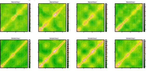
3.1 Yeast cycle data. The observed (top row) and estimated (bottom row) variance-covariance matrices by cluster. The clusters are arranged from left to right,
starting with Cluster 1. . . 58
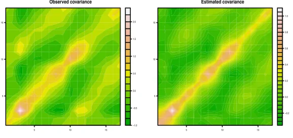
3.2 Yeast cycle data. The overall observed (left) and estimated (right) variance-covariance matrices.. . . 59
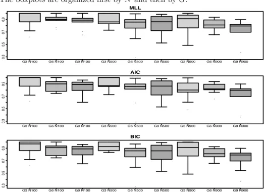
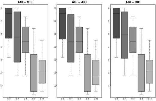
3.3 One-dimensional model. Boxplots of the ARI scores for the models selected by MLL (top), AIC (middle) and BIC (bottom). The light grey boxes correspond to G= 3, whereas the darker grey ones correspond to G = 9. The middle grey boxes correspond to G = 6. N stands for sample size. The boxplots are organized first by N and then by G.. . . 66
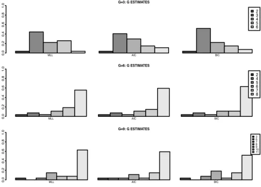
3.4 One-dimensional model. Proportion of times each criteria chose a particular number of clusters.. . . 67
3.5 Two-dimensional model. Box plots of the ARI scores for the models selected by MLL (left), AIC (middle) and BIC (right). . . 68
3.6 Two-dimensional model. Example of a dataset with six clusters . . . 69
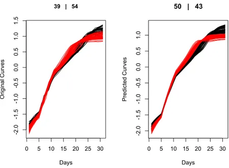
3.7 Original (left) and Predicted (right) curves for the Rats dataset . . . 70
3.8 Original (left) and Predicted (left) curves for the Growth dataset . . . 71
3.9 Model selection results for yeast cell cycle data . . . 72
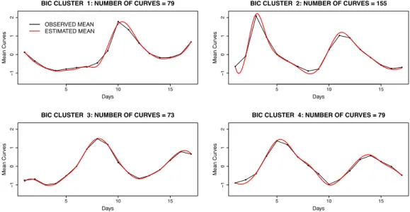
3.10 Yeast cycle data. Observed and model-estimated mean curves for the four clusters yielded by the MLL and BIC criteria . . . 73
3.11 Yeast cycle data. Observed and model-estimated mean curves for the five clusters found by Cho et al. [7] . . . 74
3.12 Yeast data. Overall mean curves (left) and distribution of the νi associated with the error term distribution of the data. . . 74
3.13 Illustration of the difference at days 40 and 42. . . 75
3.15 The M114G-partition mean curves by Wur category . . . 79
3.16 The M13G-partition mean curves by Wur category . . . 79
3.17 The M23G-partition mean curves by Experiment category . . . 81
3.18 The M12 3G-partition mean curves by Wur and Experiment for cluster 1 . . . 81
3.19 The M12 3G-partition mean curves by Wur and Experiment for cluster 2 . . . 82
3.20 The M12 3G-partition mean curves by Wur and Experiment for cluster 3 . . . 82
3.21 MLL Comparison for model selection. . . 83
4.1 Comparison of the three criteria for model selection.. . . 106
4.2 Similarity ratio and model performance.. . . 107
4.3 Influence of postulated G . . . 107
4.4 Comparison of True and estimated number of clusters . . . 108
4.5 Cluster mean curves for the three partitions found by the Bayesian Lasso clustering model. The first row displays the clusters in the two-dimensional space of functional principal components (FPC) scores. The bottom row shows the cluster mean-curves.. . . 109
DÉDICACE
Je dédie ce travail à mon épouse Ange Christelle et mes enfants Ékoué Émidèl et Ayélé Asséna.
REMERCIEMENTS
« Le temps met tout en lumière. » (Thalès)
En premier lieu et par dessus toute considération, je veux dire Merci à Dieu le Père Tout-puissant qui a permis la réalisation (et enfin, la fin) de cette thèse. À toi, Père Éternel : « Mes faibles mots te sanctifient et mon esprit te magnifie. Seigneur, je te dis Merci » (ex-trait du chant Dans ton sanctuaire de GAEL).
Plusieurs personnes ont vécu avec moi, ces longues années de doctorat.
Sur le plan familial et du haut de cette liste, je remercie ma charmante et douce épouse : « Chérie, Merci de tout coeur pour l’amour et le soutien. Merci également pour ces bonheurs immenses qui ont jalonné cette thèse, notamment ces deux magnifiques bébés ». Ensuite, je rends un vibrant hommage à mes parents, à ma très chère maman et à mon père pour leurs prières, conseils et rigueur. « C’est vous qui avez semé cette graine, l’avez arrosée et entretenue pendant toutes ces années ». Spécialement pour toi Tonton, j’ajoute ces vers de Alfred de Vigny : « A voir ce que l’on fut sur terre et ce qu’on laisse, seul le silence est grand, tout le reste est faiblesse ». Je veux également dire un gros gros Merci à ma mère Tanty et à mes soeurs chéries Amélé, Akwavi et Enyonam : « Oui, la distance nous joue des tours mais l’amour survit à tout ». Merci également à ma merveilleuse et bienveillante belle-famille au Canada et en Côte d’Ivoire.
Sur le plan académique et professionnel, j’ai beaucoup de reconnaissance et d’admiration à témoigner à mon directeur de recherche. Je n’en rajoute pas et peut-être même n’en dis-je pas assez en affirmant que je n’aurais pu rêver un meilleur directeur de thèse. « Disponible, tu as su valoriser ce qui est bien, et transformer ce qui l’est moins. Merci Alejandro pour tout ce que tu m’a appris, pour ton sens sourcilleux, ta générosité et ta sensibilité à mon contexte personnel. Ta compétence, ta rigueur scientifique et ta clairvoyance m’ont beau-coup édifié. J’aime à penser qu’au fil des années nous sommes devenus de bons amis ».
Je remercie également tous les professeurs et tout le valeureux personnel du Département de mathématique et statistique de l’Université de Montréal. Je ne saurais oublier tous mes collègues de la Direction de la modélisation des systèmes de transport du Ministère des Transports. Merci à tous pour vos encouragements notamment dans le sprint final. Et enfin, Merci à Amhos. Merci à tous mes amis. Merci à tous mes étudiants du DMS.
INTRODUCTION
Dans plusieurs domaines de recherche, notamment dans les sciences sociales, les études lon-gitudinales sont devenues un outil essentiel pour analyser l’évolution d’un phénomène donné
dans le temps, qui peut revêtir un caractère plus important que la simple connaissance du
moment d’apparition d’un tel phénomène. Elles sont constituées de mesures répétées d’une ou de plusieurs variables, prises sur un ensemble d’individus, à différents points d’un axe temporel. Une caractéristique fondamentale de ce type de données est que les observations recueillies sur un même sujet tendent à être corrélées. Il s’agit de la corrélation intra-sujet. En effet, la connaissance de la valeur observée de la variable réponse à une date donnée four-nit de l’information sur sa valeur probable à date future (voir Fitzmaurice and Ravichandran [9]). La corrélation entre les mesures répétées va à l’encontre de l’hypothèse fondamentale d’indépendance qui constitue la pierre angulaire de plusieurs techniques standard en statis-tique (test t, régression linéaire, anova). Cette particularité des données longitudinales est décrite dans plusieurs articles et ouvrages traitant du sujet et notamment dans Fitzmaurice et al. [8] qui présente également les différentes sources et nature de la corrélation dans ce type de données ainsi que les conséquences potentielles lorsque celle-ci n’est pas prise en compte dans l’analyse statistique. De plus, les données longitudinales diffèrent des autres types de données en statistique telles que les données multivariées, les études transversales, les séries temporelles, et leur analyse requiert par conséquent des méthodologies spécifiques. La méthodologie statistique d’analyse des données longitudinales a connu au cours des trente dernières années un développement considérable, qui a été facilité par l’émergence de technologies nouvelles qui favorisent les applications numériques sur des ordinateurs de plus en plus puissants. Les méthodes les plus couramment utilisées dans l’analyse des données longitudinales sont basées sur des modèles paramétriques tels que les modèles linéaires à effets mixtes proposés par Laird and Ware [14] pour l’étude des variables réponses conti-nues observées au fil du temps. Ces méthodes reposent sur une décomposition explicite de
la variation dans les données en variabilité inter et intra-sujet (Verbeke and Molenberghs [28]). La classe des modèles paramériques comprend également les modèles marginaux et les modèles linéaires généralisés à effets mixtes (McCullagh and Nelder [16]) qui sont deux généralisations importantes des modèles linéaires aux cas où la variable réponse est discrète, ainsi que les modèles non linéaires à effets mixtes. Plusieurs exemples d’applications empi-riques telles que Zeger and Diggle [32], Brumback and Rice [2], Lin and Ying [15] et Diggle et al. [5] montrent que les hypothèses paramétriques ne sont pas toujours appropriées pour modéliser la dynamique temporelle entre une variable d’intérêt et des variables explicatives dans une étude longitudinale. Ainsi, les méthodes non-paramétriques et semi-paramétriques ont émergé dans la littérature statistique afin de proposer des formes fonctionnelles plus flexibles dans l’analyse des données longitudinales. Il s’agit essentiellement d’adapter les méthodes par noyaux (Wand and Jones [30], Fan and Gijbels [6]) et les méthodes de lissage par splines (Wahba [29], Green and Silverman [11], Stone et al. [24]) qui ont été élaborées pour l’étude de données indépendantes, aux spécificités des données longitudinales notam-ment la corrélation intra-sujet entre les mesures répétées dans le temps.
Une autre méthodologie non paramétrique de la modélisation des données longitudinales est fournie par l’approche de l’analyse de données fonctionnelles (ADF) selon laquelle les mesures répétées recueillies auprès des individus sont considérées comme des portions de courbes (Ramsay and Silverman [21]). En effet, les trajectoires longitudinales sont perçues comme étant un échantillon de fonctions (ou courbes) partiellement observées sur un inter-valle de temps sur lequel elles sont souvent supposées lisses. En d’autres termes, les données longitudinales sont considérées comme des données fonctionnelles irrégulièrement observées. L’objectif de cette approche est donc d’utiliser les outils de l’analyse de données fonction-nelles pour prédire chaque trajectoire individuelle à partir des mesures effectuées, en tenant compte des mesures provenant de tous les autres individus impliqués dans l’étude longitu-dinale.
Depuis quelques années, des méthodes d’extension des techniques de l’analyse de données fonctionnelles aux données longitudinales font l’objet d’un champ de recherche en pleine expansion. L’émergence de ce nouveau paradigme repose sur l’idée fondamentale que les méthodes de l’ADF peuvent constituer un outil remarquable pour optimiser l’analyse des données longitudinales (Zhao et al. [33], Rice [22]), notamment en ce qui concerne le regrou-pement en classes (partitionnement ou classification non supervisée ou encore clustering en anglais) tel qu’illustré dans Ullah and Finch [27] qui présente les récentes applications majeures de l’approche par l’ADF. Le regroupement en classes a toujours été une méthode
d’analyse de données priviliégiée dans le cas des données longitudinales et porte sur l’identi-fication de groupes, non définis a priori et suggérés par les données, de sorte que les individus dans un même groupe tendent à être similaires dans un certain sens (défini par le critère de regroupement) et ceux dans différents groupes tendent à être non similaires. Par exemple, le partitionnement des données d’expression génétique est un enjeu important en bioinfor-matique car la compréhension des gènes qui se comportent de façon similaire conduit à la découverte d’importantes informations biologiques (McNicholas and Subedi [18]). Les tra-vaux qui s’inscrivent dans le contexte d’extension de l’ADF utilisent essentiellement l’analyse fonctionnelle en composantes principales (AFCP) qui a émergé comme un outil majeur en ADF et qui permet de réduire la dimensionalité d’un ensemble de données fonctionnelles en identifiant les modes de variation les plus significatifs. Ramsay and Silverman [21] propose une excellente présentation de la théorie de l’AFCP, des techniques de calcul des compo-santes principales telles que la discrétisation des fonctions observées et l’expansion dans une base de fonctions, ainsi qu’une étude comparative de ces différentes approches de l’AFCP. L’objectif de cette thèse est de contribuer à l’élaboration de nouveaux modèles plus flexibles, basés sur l’approche de l’analyse des données fonctionnelles pour l’analyse et le regroupe-ment en classes des données longitudinales ou des courbes d’évolution corrélées. La théorie classique de l’ADF s’intéresse aux données de dimension infinie telles que les courbes ou les images. Elle est donc essentiellement appropriée pour l’étude des données longitudinales
balançées c’est à dire des mesures prises à intervalles réguliers (grille temporelle
uniformé-ment graduée), de sorte que tous les sujets sont évalués aux mêmes périodes de temps et admettent donc le même nombre de mesures. Mais dans la réalité, la plupart des études longitudinales résultent très souvent en des données non balançées (mesures irrégulières, prises à des périodes de temps assez différentes pour les individus, et de plus, tous les sujets peuvent ne pas avoir le même nombre de mesures).
Nous présentons dans le cadre de cette thèse, deux nouveaux modèles de classification non-supervisée de données longitudinales basés sur l’approche de l’analyse des données fonction-nelles, qui tiennent compte de la forme générale des variables-trajectoires et qui constituent des contributions notoires dans la panoplie des méthodes d’analyse disponibles dans ce do-maine. Ces modèles font l’objet d’articles scientifiques et se démarquent non seulement par leur flexibilité, la pertinence et l’originalité de leurs hypothèses et lois a priori, mais aussi et surtout par le fait qu’ils sont conçus pour convenir à tous les types de données longi-tudinales, aussi bien balançées que non balançées. Par exemple, la première méthodologie proposée réalise le partitionnement de données longitudinales à partir d’une seule variable
(1D) ou de deux variables conjointement (2D) mais reste facilement extensible au regroupe-ment en classes basé sur 3 ou plus de 3 variables avec prise en compte possible d’effets fixes. Par ailleurs, une contribution majeure dans la deuxième méthodologie proposée dans cette thèse est cette idée d’utiliser une pénalisation du type Lasso comme loi a priori, dans le sens qu’au lieu de chercher le paramètre optimal Lasso, il est incorporé directement comme paramètre du modèle et il faut impérativement estimer la constante de normalisation qui lui est associée. Nous présentons également dans cette thèse, une revue assez concise de la littérature existante sur les différents modèles d’analyse et de partitionnement des données longitudinales.
Le premier chapitre non introductif de cette thèse présente un aperçu général des différentes méthodes de traitement des données longitudinales selon une perspective historico-évolutive, en examinant les approches paramétrique, semi-paramétrique et non-paramétrique. Une em-phase particulière est mise sur les méthodes et procédures de regroupement en classes (mo-dèles de clustering) qui constituent une question importante et largement discutée dans la littérature sur les données longitudinales. En effet, depuis quelques décennies, plusieurs tra-vaux méthodologiques ont porté sur l’extension aux données longitudinales, des différentes méthodes de partitionnement bien développées en matière de données indépendantes et qui ne sont pas adaptées au traitement des mesures répétées. La synthèse proposée dans ce chapitre se démarque d’autres études similaires existantes (Fitzmaurice et al. [7], Gibbons et al. [10], Jacques and Preda [12], Bouveyron and Brunet [1]) par sa diversité (différentes méthodologies selon différents angles de traitement des données longitudinales) et son inté-gration des méthodes et algorithmes de partitionnement plus récents.
Dans le deuxième chapitre de cette thèse, nous présentons le modèle flexible développé pour l’analyse et le partitionnement de données longitudinales (balancées ou non). Le modèle combine l’analyse fonctionnelle en composantes principales et le regroupement en classes, qui repose sur l’espace des coefficients dans la base des splines et un modèle de mélange de distributions de Student de degrés de liberté inconnus. Nous développons une approxima-tion de la log-vraisemblance marginale (MLL) pour la sélecapproxima-tion de modèles qui se compare favorablement aux critères usuels (AIC et BIC). Nous considérons également une extension du modèle aux courbes multidimensionnelles. Des études de simulations et de comparaison avec d’autres modèles du genre, ainsi que des applications sur des données réelles ont été menées pour évaluer la pertinence et la performance du modèle. En effet, la méthodologie a été appliquée sur plusieurs jeux de données assez connus tels que les données de rats publiées dans Crowder and Hand [4] et étudiées dans McNicholas and Murphy [17] dans un contexte longitudinal, les données de croissance provenant des études de croissance de
Berkeley (Tuddenham and Snyder [26]), les données d’activité électrique cardiaque étudiées dans Olszewski [19], l’ensemble de données génétiques sur le cycle cellulaire de Cho et al. [3] et les données sur le virus du syndrome respiratoire et de reproduction chez les porcs (voir Rowland et al. [23]). James and Sugar [13] avaient proposé un modèle similaire mais notre modèle présente l’avantage d’être plus précis et exact par rapport à la structure imposée sur les courbes individuelles et la procédure pour identifier les groupes suggérés par les données. L’estimation des paramètres est effectuée à partir de l’algorithme EM, de plus en plus utilisé et modifié en analyse de données longitudinales.
Dans le troisième chapitre, nous présentons une nouvelle procédure de partitionnement fonctionnel (functional clustering) pour l’analyse des données longitudinales. L’idée origi-nale du modèle proposé est inspirée des récents travaux dans le domaine de la sélection de variables pour le partitionnement de données à très grande dimension dont une revue est présentée par Bouveyron and Brunet [1], dans laquelle une emphase particulière est mise sur le critère de pénalisation dans la classification non supersivée. Il s’agit en effet d’introduire, à l’instar de Pan and Shen [20] et Wang and Zhou [31], des termes de pénalité du type L1
ou L∞ dans la fonction de log-vraisemblance. La méthode que nous proposons diffère de celles existantes par son approche. Au lieu de simultanément partitionner les données et en réduire la dimensionalité en déterminant les variables les plus pertinentes pour le processus de regroupement, notre procédure de partitionnement basée sur un modèle utilise l’approche fonctionnelle et une pénalisation double du type Lasso (Tibshirani [25]) pour simultanément déterminer la dimension appropriée de la base finie de fonctions (reduction de la dimension) et le nombre approprié de groupes homogènes (partitionnement). La performance et l’utilité de la procédure sont démontrées par la simulation et l’application sur des données réelles, notamment les données d’exposition des rats à la fumée de tabac dans le cadre d’études cliniques.
[1] Bouveyron, C. and C. Brunet (2014). Model-based clustering of high-dimensional data : A review. Computational Statistics and Data Analysis 71, 52–78.
[2] Brumback, B. and J. Rice (1998). Smoothing spline models for the analysis of nested and crossed samples of curves. Journal of the American Statistical Association 93, 961–976. [3] Cho, R. J., M. J. Campbell, E. A. Winzeler, L. Steinmetz, A. Conway, L. Wodicka, T. G. Wolfsberg, A. E. Gabrielian, D. Landsman, D. J. Lockhart, and R. W. Davis (1998). A genome-wide transcriptional analysis of the mitotic cell cycle. Molecular Cel L 2, 65–73. [4] Crowder, M. J. and D. J. Hand (1990). Analysis of Repeated Measures. London :
Chapman and Hall.
[5] Diggle, P. J., P. J. Heagerty, K.-Y. Liang, and S. L. Zeger (2002). Analysis of Longitudinal
Data, 2nd Ed. Oxford : Oxford University Press.
[6] Fan, J. and I. Gijbels (1996). Local Polynomial Modelling and Its Applications. London, Chapman Hall.
[7] Fitzmaurice, G., M. Davidian, G. Verbeke, and G. Molenberghs (2008). Longitudinal
Data Analysis. Chapman & Hall CRC Handbooks of Modern Statistical Methods.
[8] Fitzmaurice, G. M., N. M. Laird, and J. H. Ware (2012). Applied Longitudinal Analysis. John Wiley and Sons, Second edition.
[9] Fitzmaurice, G. M. and C. Ravichandran (2008). A primer in longitudinal data analysis.
Circulation 118, 2005–2010.
[10] Gibbons, R., D. Hedeker, and S. DuToit (2010). Advances in analysis of longitudinal data. Annual Review of Clinical Psychology 6, 79–107.
[11] Green, P. J. and B. Silverman (1994). Nonparametric Regression and Generalized Linear
Models A Roughness Penalty Approach. London, Chapman Hall.
[12] Jacques, J. and C. Preda (2014). Functional data clustering : a survey. Advances in
Data Analysis and Classification, Springer Verlag 8(3).
[13] James, G. and C. A. Sugar (2003). Clustering for sparsely sampled functional data.
[14] Laird, N. M. and J. H. Ware (1982). Random-effects models for longitudinal data.
Biometrics 38, 963–974.
[15] Lin, D. and Z. Ying (2001). Semiparametric and nonparametric regression analysis of longitudinal data. Journal of the American Statistical Association 96, 103–126.
[16] McCullagh, P. and J. A. Nelder (1989). Generalized Linear Models, 2nd Edition. Lon-don : Chapman and Hall.
[17] McNicholas, P. D. and T. B. Murphy (2010). Model-based clustering of longitudinal data. Canadian Journal of Statistics 38, 153–168.
[18] McNicholas, P. D. and S. Subedi (2012). Clustering gene expression time course data using mixtures of multivariate t-distributions. Journal of Statistical Planning and
Infe-rence 142, 1114–1127.
[19] Olszewski, R. (2001). Generalized feature extraction for structural pattern recognition in time-series data. Ph.D. thesis, Carnegie Mellon University.
[20] Pan, W. and X. Shen (2007). Penalized model-based clustering with application to variable selection. Journal of Machine Learning Research 8, 1145–1164.
[21] Ramsay, J. and B. Silverman (2005). Functional Data Analysis. New York : Springer. [22] Rice, J. (2004). Functional and longitudinal data analysis : Perspectives on smoothing.
Statistica Sinica.
[23] Rowland, R., J. Lunney, and J. Dekkers (2012). Control of porcine reproductive and respiratory syndrome (prrs) through genetic improvements in disease resistance and tole-rance. Front. in Gen. 3 :260.
[24] Stone, C., M. Hansen, C. Kooperberg, and Y. K. Truong (1997). Polynomial splines and their tensor products in extended linear modeling (with discussion). Annals of Statistics 25, 1371–1470.
[25] Tibshirani, R. (2011). Regression shrinkage and selection via the lasso : a retrospective.
Journal of the Royal Statistical Society Series B 73, 273–282.
[26] Tuddenham, R. and M. Snyder (1954). Physical growth of california boys and girls from birth to eighteen years. Universities of California Public Child Development 1, 188–364. [27] Ullah, S. and C. F. Finch (2013). Applications of functional data analysis : A systematic
review. BMC Medical Research Methodology 1471-2288, 13–43.
[28] Verbeke, G. and G. Molenberghs (2000). Linear Mixed Models for Longitudinal Data. Springer series in statistics. New York.
[29] Wahba, G. (1990). Spline Models for Observational Data. Philadelphia : CBMS-NSF Regional Conference Series, SIAM.
[30] Wand, M. P. and M. C. Jones (1995). Kernel Smoothing. London : Monographs on Statistics and Applied Probability, Chapman & Hall.
[31] Wang, S. and J. Zhou (2008). Variable selection for model-based high dimensional clustering and its application to microarray data. Biometrics 64, 440–448.
[32] Zeger, S. L. and P. J. Diggle (1994). Semiparametric models for longitudinal data with application to cd4 cell numbers in hiv seroconverters. Biometrics 50, 689–699.
[33] Zhao, X., J. Marron, and M. Wells (2004). The functional data analysis view of longi-tudinal data. Statistica Sinica 14, 789–808.
A REVIEW OF LONGITUDINAL DATA ANALYSIS
AND CLUSTERING METHODS
Abstract
We review the recent developments in longitudinal cluster analysis according to the two main approaches, non-parametric and model-based. We deemed it useful and relevant to present at first, most of the typical longitudinal data analysis methods ranging from the parametric models to the semi and non parametric ones. Then, the clustering methods are discussed. The main purpose of this review is to provide a concise, broad and readily accessible overview of the most important and available methods for analyzing and clustering longitudinal data.
Key words : Longitudinal data, model-based clustering, sparse longitudinal data,
2.1. Introduction
Longitudinal studies have become an essential tool for studying the evolution in time of a given phenomena as they play a salient role in many various research areas. Longitudinal data arises when one or more outcomes are measured at a sequence of observation times on multiple subjects (Diggle et al. [23]). For each subject, the measurements are taken at different times during a certain period leading to a sequence of observations. That funda-mental characteristic of possible correlation between observations coming from the same subject (within-subject correlation) makes longitudinal data different from other types of data in statistics (such as multivariate data, cross-sectional data, time series data) and calls for specific methodologies. For example, longitudinal data differ from classical time series data because they consist of a large number of independent trajectories that are sparsely and potentially irregularly sampled over time, rather than a few random processes that are uniformly sampled over time (Heggeseth [51]). Similarly, historical development of ideas re-lated to longitudinal studies and their advantages over cross-sectional studies are presented in many books or papers such as Rajulton [100] ; Hedeker and Gibbons [50] and Rindfleisch et al. [105].
The statistical methodology for the analysis of longitudinal data is essentially based around three axes : parametric models, non-parametric models and semi-parametric models. In the past forty years, that statistical methodology has evolved remarkably, due to increasingly so-phisticated technologies which allow numerical applications on high performance machines. Therefore, several new avenues have been explored. For example, the works of Zhao et al. [134] and Rice [103] have shown that longitudinal data can be viewed as a type of functional data. As a consequence, a non-parametric methodology for modeling longitudinal data and based on the functional data analysis (FDA) approach has emerged. In the FDA approach pioneered by Ramsay and Silverman [101], longitudinal trajectories are viewed as a sample of partially observed functions or curves on some interval where these functions are often assumed to be smooth.
In this review, we are particularly interested in an important question widely addressed in the analysis of longitudinal data : the issue of cluster analysis (Hennig et al. [52] ; Bruckers [8]). It concerns the existence of groups or clusters (or homogeneous trajectories), suggested by the data, not defined a priori, such that individuals in a given cluster tend to be simi-lar to each other in some sense, and individuals in different clusters tend to be dissimisimi-lar. The extension of cluster analysis to longitudinal data has been the focus of a lot of metho-dological work. These methods range from heuristic approaches such as k-means (Hartigan and Wong [47] ; Tarpey [117] ; Genolini and Falissard [41]), distances or dissimilarities-based
algorithms (Komarek and Komarkova [65] ; Hennig et al. [52]) to model-based procedures (Fraley and Raftery [33] ; Fraley and Raftery [35] ; James and Sugar [60]). Most methods can be categorized into one of two approaches : nonparametric and model-based methods. The first section of the this paper, along the same lines as reviews such as Fitzmaurice et al. [31] and Gibbons et al. [44], highlights the longitudinal data analysis methods ranging from the parametric models to the semi and non parametric models. We present herein the most notable developments with an emphasis on the main characteristics of each model. The second section is mainly dedicated to the review of the two clustering categories including methods based on the functional data analysis approach.
2.2. Analysis methods for longitudinal data
The most popular and extensively used methods in the analysis of longitudinal data are based on the parametric models which often contain random effects, such as the linear
mixed-effects model proposed by Laird and Ware [67] for continuous responses. The
para-metric models also include marginal models, generalized linear mixed models for discrete responses and non-linear mixed-effects models. Many examples of empirical applications such as Brumback and Rice [9], Zeger and Diggle [131], Lin and Ying [72] and Diggle et al. [23] demonstrate that parametric assumptions are not always appropriate to modelize the temporal dynamic between a response variable and covariates in longitudinal studies. Hence, non-parametric and semi-parametric methods have emerged in the statistical literature in order to propose more flexible functional forms in the analysis of longitudinal data. This mainly relates to extending and adapting kernel methods (Wand and Jones [124] ; Fan and Gijbels [29]) and smoothing splines methods (Green and Silverman [45] ; Wahba [122] ; Stone et al. [114]), originally developed for independent data, to the particularities of longitudinal data, especially the within-subject correlation among repeated measures over time. Another non parametric methodology in modeling longitudinal data is provided by the functional data analysis (FDA) approach in which the sequence of measurements collected for each individual are considered as portions of curves. The observed measurements correspond to values of a random trajectory corrupted by measurement error. The objective is to use FDA tools to predict individual trajectories from the measurements made for a subject, borro-wing strength from the entire sample of subjects (Fitzmaurice et al. [31, chap. 10]). The research associated with the extension of FDA methodology to the analysis of longitudinal data, especially the use of functional principal components analysis (FPCA), is an area in great expansion.
2.2.1. Parametric models for analysis of longitudinal data
Parametric models, which often contain random effects, represent an analysis approach commonly used by statisticians. There is a large variety of such models, depending on the type of the response variable or the objective of the statistical analysis. Amongst others, there are linear models, generalized linear models and non linear models.
2.2.1.1. Linear models for longitudinal data
Linear parametric models are essentially based on normality assumptions and are useful for continuous longitudinal data. Introduced by Laird and Ware [67], the linear mixed-effects model is probably the most popular method in this class of models. In general, a linear mixed-effects model is specified as (Verbeke and Molenberghs [121]) :
⎧ ⎪ ⎪ ⎨ ⎪ ⎪ ⎩ Yi= Xiβ+ Zibi+ ϵi bi∼ Nq(0, D) ; ϵi∼ Nni(0, Σi) b1, ...,bN, ϵ1, ..., ϵN are independent (2.2.1) where Yiis the ni-dimensional vector of measurements of the subject i with 1 ≤ i ≤ N ; and
N being the total number of subjects in the longitudinal study. Xi and Ziare respectively,
the covariates matrices of dimensions (ni, p) and (ni, q). β is a p-dimensional vector
repre-senting the fixed effects ; bi is a q-dimensional vector representing the random effects ; ϵi is
the ni-dimensional vector corresponding to the errors. The matrices D and Σirepresent the
variance-covariance matrices of random effects and errors, respectively.
Conditionally to the random effects bi, Yi has a multivariate normal distribution of mean Xiβ+ Zibiand variance-covariance matrix Σi. Unless the model is estimated using a
Baye-sian approach (Gelman et al. [39]), the parameter estimation and the inference are based on the marginal distribution of Yi which is provided by :
p(yi) =
%
p(yi|bi)p(bi)dbi.
Given the Gaussian distribution of the random effects bi, it is demonstrated that the
res-ponse vector Yiof each individual follow a multivariate normal distribution with mean Xiβ
and variance-covariance matrix Vi= ZiDZTi + Σi.
Many models are proposed in the statistical literature depending on the choice of the cova-riance structure of the errors Σi. Most models are special cases of the general model proposed
by Diggle et al. [23]. These authors propose the general linear model with the assumption that the covariance structure of the sequence of measures collected on each individual can be specified by a certain number of unknown parameters represented by the vector α. Indeed, if yi= (yi1, ..., yini) is the ni-dimensional vector of measurements of the individual i and the
vector ti= (ti1, ..., tini) represents the measurement time points, then the yiare assumed to
be realizations of independent Gaussian vectors Yi∼ Nni(Xiβ, Vi(ti, α)). The originality of
the presentation in Diggle et al. [23] relies on two important points. First, they make an ex-plicit distinction between the mean and covariance structures by stipulating Yi= Xiβ+ εi
with εi ∼ Nni(0, Vi(ti, α)). Second, they propose an additive formulation of the different
sources of random variation in longitudinal data which are : random effects, within-subject
variability and measurement errors. Formally, the vector εi and the term εij associated to
the jthmeasurement of individual i are defined as follows :
⎧ ⎨ ⎩ εi= Zibi+ Wi(ti) + ϵi εij = ZTi(j,·)bi+ Wi(tij) + ϵij; i= 1, ..., N; j= 1, ..., ni. (2.2.2) In this decomposition, the birepresent the random effects and are a set of N q-dimensional
independent Gaussian vectors with mean vector zero and covariance matrix D. The Zi(j,·)
are q-dimensional vectors of explanatory variables attached to individual measurements and represent the jthrow of the (n
i, q)-dimensional matrix Zi. The terms {Wi(tij)} represent the
within-subject serial correlation and are N independent realizations of a Gaussian stationary process of mean zero and variance σ2 with correlation function ρ(u). The ϵ
ij represent
measurement errors and are a set of M mutually independent normal random variables with mean zero and variance τ2 where M = [&N
i=1ni]. Let Ri be the (ni, ni)-dimensional
matrix with the (j, k)th element being the correlation h
ijk between Wi(tij) and Wi(tik)
defined as hijk= ρ(|tij− tik|). Let Ini be the (ni, ni)-identity matrix. The covariance matrix
of εi= (εi1, ..., εini) is defined as :
V ar(εi) = ZiDZTi + σ2Ri+ τ2Ini. (2.2.3)
With this specification of the covariance structure for longitudinal data, it is up to the analyst to introduce one or several sources of variability in the linear model according to the context of the experience or study. One can see that the linear mixed-effects model in Equation (2.2.1) corresponds to the particular case of Equation (2.2.2) where the within-subject serial correlation is omitted and a diagonal covariance structure is imposed on the measurement errors.
The inference and parameter estimation of these models (Verbeke and Molenberghs [121] ; Diggle et al. [23] ; Fitzmaurice et al. [32] ; Molenberghs and Verbeke [92] ; Fitzmaurice et al. [31]) are based on the well-known principle of maximum likelihood (ML) or the restricted maximum likelihood (REML) estimations. The REML is used to adjust the bias introduced by the maximum likelihood estimation of the covariance components.
or REML estimators. Laird and Ware [67] showed how the expectation-maximization (EM) algorithm proposed by Dempster et al. [22] can not only be applied to obtain ML estimators, but can be useful to compute REML estimators through an empirical Bayesian approach. Other alternative procedures such as the Newton-Raphson algorithm, the quasi-Newton algorithm or the simplex algorithm of Nelder and Mead (1965) are used very often. Howe-ver, a Bayesian approach through determination of the posterior probability distribution is sometimes preferred to estimate the random effects bi in the linear mixed-effects models
(Molenberghs and Verbeke [92, chap. 10]).
2.2.1.2. Generalized linear models for longitudinal data
Generalized linear models (McCullagh and Nelder [82]) are a class of regression models on the independent observations of a discrete or continuous variable. Statisticians have then developed extensions of generalized linear models for longitudinal data in order to take into account the context of correlated observations. We present three main extensions : marginal
models, generalized linear mixed-effects models and transition models.
Marginal models : In a marginal model, the regression of a response variable on some
explanatory variables and the within-subject correlation are analyzed separately according to the following assumptions :
(1) The mean of each response E(Yij|Xij) = µij depends on the explanatory variables Xij through γ(µij) = XTijβwhere γ(·) is a known link function such as the logit for
binary responses.
(2) The variance of each Yij given the covariates, is assumed to depend on the mean
through V ar(Yij|Xij) = ϕv(µij) where ϕ is a scale parameter and v is a known
variance function.
(3) The correlation between Yij and Yik is a function of the corresponding means and
additional parameters α through Cor(Yij, Yik) = ρ(µij, µik; α) where ρ is a known
function.
It is the third component of the marginal model specification, the within-subject correlation between measurements collected for the same individual, that represents the main extension of generalized linear models to longitudinal data.
Generalized linear mixed-effects models : In a certain sense, marginal models take
into account the within-subject correlation but they provide no explanation about the po-tential source of that correlation. An alternative approach that takes into account that within-subject correlation and provides its source consists in the introduction of random
effects in the model. This is the case of generalized linear mixed-effects models defined by the following assumptions :
(1) Conditionally to the random effects vector bi, the Yij are independent and have
distributions from an exponential family with a conditional mean that depends on fixed effects as well as random effects according to γ{E(Yij|bi)} = XTijβ+ZTijbiwhere
γ(·) is a known link function.
(2) The conditional variance is a function of the conditional mean through :
V ar(Yij|Xij) = ϕv{E(Yij|bi)} where v is a known variance function and ϕ is a scale
parameter known or to be estimated.
(3) The random effects bi are independent from explanatory variables Xij and follow a
multivariate normal distribution with mean zero and covariance matrix G of dimen-sion (q, q).
The interpretation of the regression parameters is distinct in the marginal models and in the generalized linear mixed-effects models due to the difference in the target of inference. Generalized linear mixed-effects models are more appropriate when the study objective is to make inference on individuals rather than on whole population (Fitzmaurice et al. [31, chap. 2]).
Transition models : In a transition model, each realization Yij of a longitudinal
se-quence Yi is defined as a function of past responses and covariates. The dependence
bet-ween repeated measures is modeled as resulting from the influence of past values on the present observation. Thus, in transition models, one assumes that γ (E{Yij|Xij,Hij}) = XT
ijβ+
&s
r=1αrηr(Hij), where Hij = (Yi1, ..., Yij−1) represents the history of measures
col-lected before the jth occasion, and the η
r are known functions (often linear but not
neces-sarily). With generalized linear mixed-effects models and transition models, it is possible to estimate unknown parameters using traditional maximum likelihood methods (Diggle et al. [23]). The most commonly used methods for estimation in generalized linear mixed-effects models are : maximum likelihood (ML), penalized quasi-likelihood (PQL) and Monte Carlo Markov chain methods (MCMC). For example, to obtain ML estimates, the numerical in-tegration or the Monte Carlo inin-tegration is combined to optimization algorithms such as Newton-Raphson, Fisher Scoring or EM algorithm (Fitzmaurice et al. [31]). For parameter estimation in marginal models, the most commonly used approach is the generalized es-timating equations (GEE) method developed by Zeger and Liang [132]. Molenberghs and Verbeke [92] present a standard iterative procedure for estimation using GEE.
2.2.1.3. Non-linear models for longitudinal data
Non-linear models are an important class of longitudinal data analysis models. Unlike ge-neralized linear models where a certain restricted form of non-linearity can be introduced through the link function, non-linear models are fundamentally non-linear. Indeed, in mar-ginal and generalized mixed-effects models, a non-linear link function γ(·) determines an appropriate scale on which the transform of the mean of a measurement Yij is linear in the
regression parameters (and random effects according to the underlying model). However, in a non-linear model, the concept of linear predictor is abandoned and one obtains, in the case of marginal model for example :
E(Yij|Xij) = η(Xij, β), (2.2.4)
where η(·) is an arbitrary function of covariates and parameters. All three types of genera-lized linear models can be extended to non-linear models. Mixed-effects non-linear models are the most commonly used. An excellent description of those models is presented in Mo-lenberghs and Verbeke [92] and Fitzmaurice et al. [31].
2.2.2. Non-parametric and semi-parametric models for longitudinal data analysis
In longitudinal data analysis, one is usually interested in the estimation of the underlying curve that generate the observed measures. For that purpose, parametric models are very often proposed. However, the main problem with parametric modeling is the quest of a suitable model with a limited number of parameters and that is the best fit to the data. Furthermore, these models suffer from an inflexibility to analyze structures sometimes very complicated and challenging in longitudinal data. It would then be more appropriate that the relationship between the mean of a response variable and covariates does not rely completely on parametric assumptions. Non-parametric and semi-parametric models then represent an alternative to parametric models and have encountered very significative developments in the past years. Non-parametric and semi-parametric models for independent data have then been extended to longitudinal data where the presence of within-subject correlation is a major challenge to take up.
Let’s consider a longitudinal study with a single explanatory variable X. Let (Yij, Xij) be the
dependent variable and the covariate for individual i (i = 1, ..., N) measured at time point tij
(j = 1, ..., ni). The dependent variable can be continuous or discrete. The marginal mean and
the marginal variance of Yij are given by : µij = E(Yij|Xij) and V ar(Yij|Xij) = ϕ−1v(µij)
mean depends on Xij according to :
γ(µij) = θ(Xij), (2.2.5)
where θ(·) is an unknown smooth function and γ(·) is a known link function. The commonly used link functions include the identity link [γ(µ) = µ] for Gaussian realizations ; the logit
link [γ(µ) = log{µ/(1 − µ)}] or the probit link [γ(µ) = Φ−1(µ)] for binary realizations
(Φ is the cumulative distribution function of a Gaussian distribution) ; and the log link [γ(µ) = log(µ)] for Poisson type realizations. Among non-parametric models, which are distinct according to the method of estimation of the θ function, there are models based on kernel methods and models based on spline methods.
2.2.2.1. Kernel-based non parametric methods
There are two main methods : the local polynomial kernel generalized estimating equations (GEE) estimator and the kernel-seemingly unrelated estimator (kSUR). The LPK-GEE estimator (Lin and Carroll [73]) is an extension of the conventional local polynomial kernel (Fan and Gijbels [29]) estimator to longitudinal data through the introduction of a covariance matrix in a way similar to the method of generalized estimating equations for generalized linear models. Specifically, at a target point x, θ(Xij) is locally approximated
by a dth-order polynomial as :
θ(Xij) ≈ α0+ · · · + αd(Xij− x)d= XTi(j,·)α (2.2.6)
where Xi(j,·) = {1, ..., (Xij − x)d} and α = (α0, ..., αd)T. The estimation equation of the
symmetric LPK-GEE estimator is :
N ' i=1 XT i∆iK1/2ih V−1i K 1/2 ih {Yi− µi} = 0 (2.2.7)
where Xi is the matrix whose jth row is Xi(j,·); ∆i = diag{δij} with δij = 1/γ′(µij) ; Kih = diag{Kh(Xij− x)}. Note that Kh(s) = h−1K(s/h) where h is a bandwidth and K(·)
is a kernel function that is often chosen as a symmetric probability density function of mean zero. The matrix Viis a “working” covariance matrix defined as Vi=
(
S1/2i Ri(ξ)S1/2i
) with
Si = diag{ϕ−1v(µij)} and Ri is an invertible correlation matrix, which possibly depends
on a vector of parameters ξ that can be estimated using the method of moments. Also,
µi = {µi1, ..., µini}T with µij = γ−1(XTi(j,·)α). Most commonly used kernel functions K(·)
include the Gaussian kernel, the uniform kernel and the Epanechnikov kernel.
Note that Ri is a user-specified working correlation matrix. It is used to account for the
within-subject correlations of responses and to estimate the true correlation structure which is unknown. The three most common used working correlation structures are Independent
(Cor(Yij, Yik) = 0, j ̸= k), Exchangeable or Compound symmetry (Cor(Yij, Yik) = ρ, j ̸= k)
and AR(1) or First-order autoregressive (Cor(Yij, Yik) = ρ|j−k|, j ̸= k). Hu et al. [54], among
others, discussed the choice of a good working correlation structure and develop a nonpa-rametric and data-adaptive method for selecting the correlation structure.
Equation (2.2.7) can be solved using the Fisher Scoring algorithm via iteratively re-weighted least squares. Let ˆα be the solution of that equation. Then, the estimator LPK-GEE of θ(x) is ˆθK(x) = ˆα0. Lin and Carroll [73] have also considered a non-symmetric LPK-GEE
es-timator by replacing (K1/2ih V−1i K 1/2 ih ) by (V−1 i Kih )
and the asymptotic performance of the estimator is similar to the symmetric case. In Chen and Jin [15], the authors have propo-sed an improved version of the LPK-GEE estimator which uses a degenerate local working covariance matrix. Unlike the original LPK-GEE estimator which is more efficient while the within-subject correlation is ignored (Wu and Zhang [127]), the efficiency of the kernel estimator of Chen and Jin [15] is the same, no matter whether one ignores correlation or accounts for correlation.
A heuristic explanation concerning the failure of the LPK-GEE estimator to efficiently account for the within-subject correlation is that it is based on the principle of local likeli-hood (Fitzmaurice et al. [31, chap. 9]). The design of a kernel-based estimator that accounts for the correlation in longitudinal data should then not rely on the traditional local likeli-hood. Thus, Wang [125] proposed the kernel-based seemingly unrelated (kSUR) estimator. Specifically, let’s consider a dth-order polynomial kernel estimator using the approximation
in Equation (2.2.7). If ˆθ[l]
K(x) represents the kSUR estimator of θ(x) at the lthiteration, then
at the (l + 1)thiteration, one has ˆθ[l+1]
K (x) = ˆα0where ˆα = (ˆα0,ˆα1, ...,ˆαd)Tis solution to the
following equation : N ' i=1 ni ' j=1 Kh(Xij− x)XTiV−1i {Yi− µi(j)} = 0. (2.2.8)
In Equation (2.2.8), Vi is the working covariance matrix ; Xi is a (ni, d+ 1)-dimensional
matrix of zeros except at the jth row which is {1, (X
ij− x), ..., (Xij− x)d}T; Khis a kernel function and µi(j) = * ˆθ[l] K(Xi1), ..., ˆθ[l]K(Xi,j−1), d ' k=0 (Xij− x)kαk, ˆθ[l]K(Xi,j+1), ..., ˆθ[l]K(Xini) +T .
The kSUR estimator ˆθ∗
K(x) = ˆα0 is obtained at the convergence. The Fisher Scoring
algo-rithm can be used to iteratively solve Equation (2.2.8). The kSUR estimator is convergent and effectively accounts for the within-subject correlation. Simulation results showed that it is more efficient than the kernel-based GEE estimator in term of the quadratic mean
error (Wang [125]). Lin and Carroll [75] have extended the kSUR method to the likelihood principle.
2.2.2.2. Splines-based non parametric methods
An alternative method to non-parametrically estimate the function θ(x) in Equation (2.2.5) consists in the use of smoothing splines. A smoothing spline estimates the non-parametric regression function θ(x) using a piecewise polynomial function with all the observed covariate values Xiused as knots, where smoothness constraints are assumed at those knots (Wahba
[122], Green and Silverman [45]). For longitudinal data, there are essentially, the generalized smoothing splines estimator, the P-splines estimator and the regression splines estimator. To illustrate key features of the generalized smoothing splines estimator, let’s consider the Gaussian realizations (identity link), thus the model :
Yij= θ(Xij) + ϵij, (2.2.9)
where the ϵi = (ϵi1, ..., ϵini)
T are independent with zero mean and covariance matrix Σ.
By assuming a working covariance matrix Vi, the rth-order smoothing splines estimator
minimizes −2N1 N ' i=1 {Yi− θi}TV−1i {Yi− θi} − 1 2λ % {θ(r)(x)}2dx (2.2.10) = −2N1 'N i=1 {Yi− θi}TV−1i {Yi− θi} − 1 2λθTΩθ (2.2.11)
where θi = {θ(Xi1), ..., θ(Xini)} ; λ is a tuning parameter controlling the trade-off between
the fitting quality and smoothing level of the curve θ(·) ; Ω is the smoothing matrix (Green and Silverman [45]). Consequently, the rth-order smoothing splines estimator of θ(x) is :
ˆθS = ( ˜V−1+ NλΩ)−1V˜−1Y , (2.2.12)
where ˜V = diag(V1, ...,VN) and Y = (YT1, ...,YTN)T. Lin et al. [76] have studied the
theo-retical properties of the smoothing splines estimator and demonstrated that it is asympto-tically equivalent to the kernel SUR estimator. Their results indicated that the generalized smoothing splines estimator is a higher order kernel SUR estimator (for example, the cubic smoothing splines estimator (r = 2) is a fourth-order kernel SUR estimator). In addition, the generalized smoothing splines estimator is convergent and the most efficient estimator ˆθS is obtained when the within-subject correlation is accounted for.
Smoothing splines use all measurement points as knots. Hence, for very large datasets their computations can be long and complex. Regression splines (Stone et al. [114]) that use a small number of knots have been proposed for non-parametric regression on longitudinal
data under the model in Equation (2.2.9) (Rice and Wu [104] ; Huang et al. [56]). A regres-sion spline approximates θ(·) by θ(x) =&L
l=0Bl(x)αlwhere the number of knots is small and
{Bl(·)}Ll=0 is a set of L basis functions such as B-splines. The coefficients αl are estimated
by weighted least squares.
Another alternative consists in using the P-splines (Eilers and Marx [26] ; Ruppert et al. [107]) that require a moderate number of knots (usually smaller than the sample size but greater than the number of knots in the regression splines case). If {(x−x1)3+, ...,(x−xM)3+}
refers to a plus functions basis built from the M knots x1, ..., xM (a+ = a if a > 0 and 0
otherwise), then θ(·) can be approximated by
θ(x) = α0+ α1x+ α2x2+ α3x3+ M ' m=1 (x − xm)3+αm+3= B(x)Tα (2.2.13) where B(x) = {1, x, x2, x3,(x − x
1)3+, ...,(x − xM)+3}T and α = (α0, ..., αM)T. Note that
in this case, L = M + 3 + 1. Under the model in Equation (2.2.9), the coefficients α are estimated using the penalized log-likelihood.
2.2.2.3. Semi-parametric methods
Semi-parametric models have parametric as well as non-parametric components. Let’s as-sume that Yij is the jth measurement (j = 1, ..., ni) of individual i (i = 1, .., N). Equation
(2.2.14) represents a marginal semi-parametric model where Xij is a p-dimensional vector
of covariates whose effects are modeled parametrically and Wij is another scalar covariate
whose effects are modeled non-parametrically. Specifically,
γ(µij) = Yij= XTijβ+ θ(Wij) (2.2.14)
where γ(·) is a known link function and θ(·) is an unknown smooth function as in Equation (2.2.5). Following Zeger and Diggle [131], Lin and Carroll [74] have studied the model of Equation (2.2.14) by first estimating θ(·), given β, using the non-parametric method LPK-GEE. Then, given the resulting local polynomial kernel GEE estimator of θ(·) denoted by ˆθ(w; β) and equal to ˆα0 (defined as in Section 2.2.2.1), the regression coefficients β
are estimated through the profile method which consists in solving the profile estimating equation : N ' i=1 ∂µTi ∂β V −1 i [Yi− µi] = 0, (2.2.15)
where ˆθi = {ˆθ(Wi1; β), ..., ˆθ(Wini; β)}T; Vi is a working covariance matrix and µi is the
vector whose jth component is µ