HAL Id: hal-02442917
https://hal.univ-lorraine.fr/hal-02442917
Submitted on 23 Oct 2020
HAL is a multi-disciplinary open access
archive for the deposit and dissemination of
sci-entific research documents, whether they are
pub-lished or not. The documents may come from
teaching and research institutions in France or
abroad, or from public or private research centers.
L’archive ouverte pluridisciplinaire HAL, est
destinée au dépôt et à la diffusion de documents
scientifiques de niveau recherche, publiés ou non,
émanant des établissements d’enseignement et de
recherche français ou étrangers, des laboratoires
publics ou privés.
Djerioui Ali, Azeddine Houari, Abdelhakim Saim, Mourad Aït-Ahmed, Serge
Pierfederici, Mohamed Fouad Benkhoris, Mohamed Machmoum, Malek
Ghanes
To cite this version:
Djerioui Ali, Azeddine Houari, Abdelhakim Saim, Mourad Aït-Ahmed, Serge Pierfederici, et al..
Flat-ness Based Grey Wolf Control for Load Voltage Unbalance Mitigation in Three-Phase Four-Leg Voltage
Source Inverters. IEEE Transactions on Industry Applications, Institute of Electrical and Electronics
Engineers, 2019, �10.1109/TIA.2019.2957966�. �hal-02442917�
Flatness Based Grey Wolf Control for Load Voltage Unbalance
Mitigation in Three-Phase Four-Leg Voltage Source Inverters
Ali DJERIOUI(a) (b), Azeddine HOUARI(b), Abdelhakim SAIM(c)(b), Mourad AIT-AHMED(b), Serge PIERFEDERICI(d), Mohamed Fouad BENKHORIS(b),
Mohamed MACHMOUM(b), Malek GHANES(e)
(a) LGE, Laboratoire de Génie Electrique, University Mohamed Boudiaf of M'Sila, BP 166 Ichbilia, MSila, Algeria (b) IREENA - Institut de Recherche en Energie Electrique de Nantes Atlantiques Saint-Nazaire, France
(c) the Department of Instrumentation and Control, University of Sciences and Technology Houari Boumediene, 16111 Algiers, Algeria (d) The laboratoire d’Energétique et de Mécanique Théorique et Appliquée, École Nationale Supérieure d’Électricité et de Mécanique, Université de Lorraine, Nancy, France
(e) Ecole Centrale de Nantes, LS2N UMR CNRS 6004, 44321 Nantes , France Email: ali.djerioui@univ-msila.dz, Azeddine.Houari@univ-nantes.fr
Abstract -- Standalone power-supply systems become a key
solution to effectively address load demand in remote locations wherein the voltage asymmetry raises as a particular concern in view of the large number of single phase household and communities loads. Over these loading conditions, the use of Four-Leg Voltage Source Inverters (FL-VSIs) appears as a suitable topology to provide clean power with symmetrical voltage waveforms. The reported work employs the differential flatness theory associated with Grey Wolf optimization in order to guarantee proper operations of the FL-VSIs in different loading conditions. In fact, the differential flatness theory is applied to check the flatness of the FL-VSIs, which allows implementing a reduced control model. Then, a Grey Wolf algorithm which acts as a tracking controller (GWC) is developed. The GWC generates an optimal control signal used by the differentially flat model so as to ensure adequate control performance, even under severe load disturbances and model inaccuracies. A comprehensive experimental test is carried out to validate the effectiveness of the proposed flatness based grey wolf controller (FB-GWC).
Index Terms-- Standalone Microgrids, Voltage unbalance,
Four-Leg Voltage Source Inverter (FL-VSI), Differential flatness, Grey Wolf optimization.
I. INTRODUCTION
The output voltage quality in standalone power-supply systems is gaining more attention with regards to the increasing penetration of distributed renewable energy resources [1][2]. However, the integration of such power sources as distributed generation entities must to comply with many technical and performance requirements [3-5]. Accordingly, a number of regulatory and grid considerations refer to power quality in standalone power-supply applications. Among them, European standard EN 50160 states that the allowable variation of supplying voltages cannot exceed 10% of their nominal values. The voltage harmonic content quantified by the total harmonic distortion index (THD) must, according to IEEE standard 519-1992 and recently 1547-2014, not exceed 5%. Furthermore; the voltage
unbalance factor (VUF) should be in compliance with the IEC standards and kept below 2% as long as the consumers’ current does not include which essentially characterizes the prevalence of single-phase loads in three-phase four-wire electrical networks [6-12]. Indeed, the unbalanced loading can represent a large extent of the total load scenario in standalone microgrid configurations wherein the voltage asymmetry raises as a particular concern in view of the large number of single phase household and communities loads [13][14].
In this context, the use of FL-VSIs as power source conversion units or even as power quality conditioners appears as a suitable topology to maintain balanced sinusoidal output voltage waveforms over all loading conditions in transformer-less applications [15]. Compared to three phase three leg inverters with split DC-links, the addition of the fourth leg provides numerous extra advantages in terms of voltage rating. Indeed, reduced DC bus voltage is involved and larger AC voltage may be supported (over 15%) since it requires a reduced DC bus voltage and can support larger AC voltages (over 15%) [10]. Moreover, the additional fourth leg provides a path to draw zero current sequences, which sustains the converter capability to handle critical load conditions, such as the presence of single-phase or unbalanced phase loading [16]. FL-VSIs are widely used in different standalone and grid connected applications, namely distributed generation [17] with grid connected [18], standalone [13] and uninterruptible power supply mode of operation [19]: active power filtering [20-22], including distributed static compensators [23] and dynamic voltage restorers [24].
Nevertheless, the control of such converter in standalone power-supply applications represents a quite complicated task and, therefore, an advanced control strategy has to be designed. The control strategy synthesis must have three main objectives, tracking performances, disturbance rejection
and load voltage unbalance compensation. For this purpose, many control schemes have been previously analyzed in different reference frames. They focus on control of load voltage and must meet power sharing and quality requirements in power applications based FL-VSIs under unbalanced and various load conditions. In this way, a number of research contributions proposes classical control strategies, with proportional integral (PI) and proportional resonant linear regulators [23][25]. The obtained test results demonstrates the effectiveness and the simplicity of these controllers. However, their dynamic responses show sluggish performances in transients modes even more when cascaded control schemes are employed [26-28]]. An undesirable feature of these control schemes is the introduction of a decoupled control, which increases the control complexity, and correspondingly the computational load [15][25]. To deal with linear regulators limitations, several nonlinear control methods are proposed in the literature including feedback linearization control [21][29], backstepping [20][30] and sliding mode control [19]. These control methods use differentiation to achieve the control law, which results in high order derivative control terms. These derivatives can affect the control law capabilities under severe load disturbances and model inaccuracies.
Among the reported control strategies, the flatness-based control (FBC) appears as an interesting nonlinear control approach due to its useful performances when explicit trajectory planning is required under different operating conditions [31]. Indeed, the flatness theory allows an accurate description of the transient and the steady state dynamic of the overall system state variables based on differentially flat outputs. In addition, and as reported in various works [32-36], the FBC demonstrates stable performances even under large operating point and system parameters variation. For instance, the use of FBC has been proposed for three phase three leg VSIs and its effectiveness has been highlighted through comparisons with both proportional integral and feedback linearization controllers [34]. Also, the control of parallel three-phase VSIs is proposed in [35], where the flatness theory is used with the aim to minimize the effect of circulating currents and reduce voltage distortion at the Point of Common Coupling (PCC). A literature review of the main properties and applications of the FBC in power systems is proposed in [36].
More recently, optimization based control methods like model predictive controllers (MPC) and optimal linear quadratic regulators (LQR) emerge as effective tools [31][32]. For instance in [31], a MPC strategy is proposed for FL-VSI, wherein the minimization of a cost function yields the inverter optimal switching state to apply at the next sampling instant. This strategy presents relevant
performances, but suffers from a variable switching frequency. Moreover, the fourth leg operates at higher switching frequency than the phase legs, which complicates the output filter design as well as the neutral inductor sizing. In [32], a Particle Swarm Optimization (PSO) algorithm is proposed to on-line adapt the weighting matrices (Q and R) of an LQR controller. Besides the interesting performance of the proposed strategy, it can be mentioned that under severe nonlinear condition, the PSO technique can fall into local optimum, which can alter the control performances.
In this paper, a novel control strategy is proposed for FL-VSI based standalone power supply systems. The proposed strategy combines the advantages of flatness control and optimization. Indeed, a FBC controller is designed and extended with an evolutionary search algorithm that acts as a tracking controller to achieve the desired power quality requirements. The use of a Grey Wolf (GW) algorithm is preconized since it presents several advantages for practical implementation in terms of low computing complexity, and convergence accuracy [37]. The GW algorithm is used to search for an optimum correction of the flat output references in such a way to secure the desired trajectory tracking performances especially in the presence of substantial nonlinear and/or unbalanced loads.
The main contributions of this work are summarized as follows.
1) A FBC is extended with a GW optimization algorithm to enhance the control performance of an LC-L interfaced FL-VSI in presence of disturbing loads such as single-/three- phase, unbalanced, and nonlinear loads.
2) The GW algorithm depends on few parameters (weighting factors) that are tuned in order to minimize the voltage THD and VUF. The GW algorithm is used to minimize a cost function and generate the convenient control correction signal. 3) The robustness of the proposed controller is studied
for large load disturbances and model parameters variations.
This paper is organized as follows. In Section II, the model of the studied system is presented, and, in Section III, the design methodology of the proposed FB-GWC is detailed. Section IV present the experimental results and discuss the effectiveness of the proposed approach. Finally, section V underlines the contributions of this work.
II. SYSTEM DESCRIPTION AND MODELING
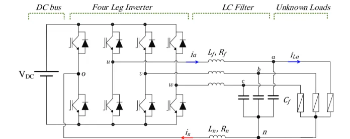
The typical circuit configuration of FL-VSIs with an output LC filter stage is depicted in Fig. 1. The DC-link is assumed as a constant voltage source. A neutral line inductor Ln is
used to connect the midpoint ‘o’ of the fourth leg to the neutral point ‘n’ of the load bus with the aim to the neutral line current ripples [14].
For the sake of simplicity, the following voltage and current vectors are defined:
Inverter voltages vector 𝒗𝒊= [𝑣𝑢𝑜, 𝑣𝑣𝑜, 𝑣𝑤𝑜]𝑇, output voltages
vector 𝒗𝒇= [𝑣𝑎𝑛, 𝑣𝑏𝑛, 𝑣𝑐𝑛]𝑇, line currents vector 𝒊𝒇=
[𝑖𝑎, 𝑖𝑏, 𝑖𝑐]𝑇,neutral current vector 𝐢𝐧= [𝑖𝑛, 𝑖𝑛, 𝑖𝑛]𝑇and load
currents vector 𝒊𝑳_𝒂𝒃𝒄= [𝑖𝐿𝑎, 𝑖𝐿𝑏, 𝑖𝐿𝑐]𝑇.
Note: Matrices and vectors are denoted with bold letters.
By applying Kirchhoff’s laws for voltage and current, to the nodes given in Fig. 1, the following load dynamics equations (1) and (2) can be obtained, where the filter line currents 𝒊𝒇
and the output voltage 𝒗𝒇 are considered as the state
variables. 𝒗𝒊= 𝒗𝒇+ 𝑅𝑓𝒊𝒇+ 𝐿𝑓 𝑑𝒊𝒇 𝑑𝑡 + (𝑅𝑛𝒊𝒏+ 𝐿𝑛 𝑑𝒊𝒏 𝑑𝑡) (1) 𝐶𝑓 𝑑𝒗𝒇 𝑑𝑡 = 𝒊𝒇− 𝒊𝑳_𝒂𝒃𝒄 (2)
After straightforward Park’s transformation P(θ) the system state equations are obtained in the synchronous reference frame:
𝒙̇ = 𝑨 𝒙 + 𝑩 𝒖 + 𝑪 𝒅 (3) with: 𝒙 = [𝑖0, 𝑖𝑑, 𝑖𝑞, 𝑣𝑐0, 𝑣𝑐𝑑, 𝑣𝑐𝑞]𝑇 the state variables vector. 𝒖 = [𝑢0, 𝑢𝑑, 𝑢𝑞]𝑇 is the 0dq-components of the input vector.
The 0dq-components of the load currents is defined by 𝒅 = 𝒊𝑳= [𝑖𝐿0, 𝑖𝐿𝑑, 𝑖𝐿𝑞]𝑇, and 𝑨 = [ − 𝑅𝑓+3𝑅𝑛 𝐿𝑓+3𝐿𝑛 0 0 −1 𝐿𝑓+3𝐿𝑛 0 0 0 −𝑅𝑓 𝐿𝑓 𝜔 0 −1 𝐿𝑓 0 0 −𝜔 −𝑅𝑓 𝐿𝑓 0 0 −1 𝐿𝑓 1 𝐶𝑓 0 0 0 0 0 0 1 𝐶𝑓 0 0 0 𝜔 0 0 1 𝐶𝑓 0 −𝜔 0] , 𝑩 = [ 1 𝐿𝑓+3𝐿𝑛 0 0 0 1 𝐿𝑓 0 0 0 1 𝐿𝑓 0 0 0 0 0 0 0 0 0 ] , 𝑪 = [ 0 0 0 0 0 0 0 0 0 −1 𝐶𝑓 0 0 0 −1 𝐶𝑓 0 0 0 −1 𝐶𝑓]
A carrier based PWM technique presented in [38], where the block diagram is shown in Fig .2, has been considered in this work due to its performance and ease of implementation. The input voltage references of the three principal phases with respect to the fourth-leg are denoted respectively: 𝑣𝑎
𝑟𝑒𝑓
, 𝑣𝑏𝑟𝑒𝑓 and 𝑣𝑐
𝑟𝑒𝑓
. The forth leg reference voltage named offset voltage is calculated with respect to the DC bus fictive middle point: 𝑣𝑛
𝑟𝑒𝑓
. Then, the reference voltages (𝑣𝑎𝑀
𝑟𝑒𝑓
, 𝑣𝑏𝑀𝑟𝑒𝑓, 𝑣𝑐𝑀 𝑟𝑒𝑓
), as illustrated in Fig 2, with respect to the fictive DC midpoint are defined as:
𝑣𝑥𝑀𝑟𝑒𝑓= 𝑣𝑥 𝑟𝑒𝑓
+ 𝑣𝑛 𝑟𝑒𝑓
, 𝑥𝜖{𝑎, 𝑏, 𝑐} (4) The offset voltage 𝑣𝑜𝑀∗ can be calculated by
𝑣𝑛 𝑟𝑒𝑓 = 𝑚𝑖𝑑(−𝑣𝑚𝑎𝑥 2 , − 𝑣𝑚𝑖𝑛 2 , − 𝑣𝑚𝑎𝑥+ 𝑣𝑚𝑖𝑛 2 ) (5)
i
ɑV
DCn
i
LɑLƒ
,
Rƒ
Cƒ
Ln , Rn
i
no
u v w a b cDC bus
Four Leg Inverter
LC Filter
Unknown Loads
where: 𝑣𝑚𝑎𝑥= 𝑚𝑎𝑥 (𝑣𝑎 𝑟𝑒𝑓 , 𝑣𝑏𝑟𝑒𝑓, 𝑣𝑐 𝑟𝑒𝑓 ) and 𝑣𝑚𝑖𝑛= 𝑚𝑖𝑛 (𝑣𝑎 𝑟𝑒𝑓 , 𝑣𝑏𝑟𝑒𝑓, 𝑣𝑐 𝑟𝑒𝑓 ). Offset voltage Generator ref va vbref vcref + + + vdc/2 -vdc/2 Sa Sb Sc Sn + + + vnref
Fig .2. Carrier based PWM technique [38]
III.PROPOSED CONTROL APPROACH
This section presents the design methodology of FB-GWC. As shown in Fig.3, the proposed voltage mode control strategy is subdivided into two main parts. The first part in which the differential flat model of the FL-VSI is used to derive the control inputs as function of the candidate flat outputs references and their successive derivatives. Meanwhile, the second part considers the use of a GW based controller to search for an optimum correction of the flat output references in such a way to ensure desired trajectory tracking performances especially in the presence of substantial nonlinear and/or unbalanced loads.
In the following, the flatness parameterization principle is first given, and then it is applied to check the flatness of the studied system. Afterward, the principle of the GW based tracking controller is provided. The end of this section summarizes the control flow implementation.
Flat Model Grey Wolf Tracking Controller System u y .. Trajectory Generator y(ƒ )+ y -Ref y(ƒ ) Ref . y(ƒ ) Ref, y(ƒ ) .Ref y(ƒ ) , Ref u =Ѱ ( ,y..)
Fig. 3. Block diagram of the proposed FB-GWC.
A. Flatness description
The differential flatness is a structural property of some controllable dynamic systems. The property allows an explicit parameterization of both system inputs and states variables as function of a set of specified variables, commonly known as flat outputs, and a finite number of their time derivatives without requiring the resolution of differential equations [34].
In other words, the general system model 𝒙̇ = 𝑓(𝒙, 𝒖) is considered as a flat system if its corresponding states vector 𝒙 ∊ ℝ𝑛 and input vector 𝒖 ∊ ℝ𝑚 can be basically expressed
as function of the candidate flat outputs given by:
𝒚 = Λ(𝒙, 𝒖, 𝒖̇, … , 𝒖(𝑝)) , 𝒚 ∊ ℝ𝑚 (6)
Accordingly, the system variables should take the form: 𝒙 = Υ(𝒚̇, 𝒚̈, … , 𝒚(𝑟)) (7)
𝒖 = 𝜳(𝒚, 𝒚̇, 𝒚̈, … , 𝒚(𝑟+1)) (8) The flatness property is more useful if the candidate flat outputs correspond to the physical outputs of the system. In this way, the flatness-based description of most of power applications has gained in importance due to the existence of numerous output candidates having with straight mathematical and physical significance. The expressions given by (7) and (8) concord with the flatness property and allow a simple calculation of feed forward control law according to the desired flat outputs trajectories. The control law is finally designed to satisfy the control objectives and guarantee that the trajectories of the inputs and outputs are smooth.
B. Flatness of the studied system
Following the control objectives, the dq-axes energies presenting the electrostatic energy stored in the capacitor filters 𝐶𝑓 and the homopolar output voltage 𝑣𝑐0 are proposed
to be the flat output candidates. Then, the flat output vector 𝐲 can be expressed as follow:
𝒚 = [ 𝑦0 𝑦𝑑 𝑦𝑞 ] = [ 𝑣𝑐0 1 2𝐶𝑓𝑣𝑐𝑑 2 1 2𝐶𝑓𝑣𝑐𝑞 2 ] (9)
According to part A, the parameterization (7) consists in the formulation of all system state variables as a function of the candidate flat output components and their respective derivatives. Regarding the proposed flat output vector (9), the 0dq-components of the output voltage can be expressed as follow: 𝒗𝒄= [𝑣𝑐0, 𝑣𝑐𝑑, 𝑣𝑐𝑞]𝑇= [𝑦0, √ 2𝑦𝑑 𝐶𝑓 , √ 2𝑦𝑞 𝐶𝑓 ]𝑇 (10)
After a derivation of the flat output vector (9), the 0dq-components of the line current can be expressed as:
𝒊 = 𝐶𝑓 𝑑 𝑑𝑡𝒗𝒄+ [ 0 0 0 0 0 −𝜔 0 𝜔 0 ] 𝒗𝒄+ 𝒊𝑳 (11) where 𝑑 𝑑𝑡𝒗𝒄 = [𝑦̇0, 𝑦̇𝑑 √2𝑦𝑑𝐶𝑓, 𝑦̇𝑞 √2𝑦𝑞𝐶𝑓] 𝑻
Notice that 𝑖𝐿 is an external disturbance.
The last step to rule on the flatness of the studied system is to verify that the input vector can be parameterized as a function of the candidate flat output components and their successive derivatives. Regarding the differential equation of the system given in (3) and the expressions of the state variables defined in (10) and (11), the input vector 𝒖 = [𝑢0, 𝑢𝑑, 𝑢𝑞]𝑇 can be
𝒖 = 𝒗𝒄+ [ 𝑅𝑓+ 3𝑅𝑛 0 0 0 𝑅𝑓 𝐿𝑓𝜔 0 −𝐿𝑓𝜔 𝑅𝑓 ] 𝒊 + [ 𝐿𝑓+ 3𝐿𝑛 0 0 0 𝐿𝑓 0 0 0 𝐿𝑓 ] 𝑑 𝑑𝑡𝒊 (12) where the expression of the theoretical line current derivation term is given in relation (12).
𝑑 𝑑𝑡𝒊 = 𝑑2 𝑑𝑡2𝒗𝒄+ [ 0 0 0 0 0 −𝜔 𝐶𝑓 0 𝜔 𝐶𝑓 0 ] 𝑑 𝑑𝑡𝒗𝒄+ 𝑑 𝑑𝑡 𝒊𝑳 (13) with : 𝑑 2 𝑑𝑡2𝒗𝒄= [ 𝑦̈0 𝑦̈𝑑 √2𝑦𝑑𝐶𝑓− 𝑦̇𝑑2 2𝑦𝑑√2𝑦𝑑𝐶𝑓 𝑦̈𝑞 √2𝑦𝑞𝐶𝑓− 𝑦̇𝑞2 2𝑦𝑞√2𝑦𝑞𝐶𝑓]
Regarding Eq. 10, 11, 12 and 13, the input vector can be parameterized as a function of the candidate flat output components and their successive derivatives.
𝒖 = 𝜳(𝒚, 𝒚̇, 𝒚̈) (14) To conclude, the studied system fulfills the flatness conditions expressed in (7) and (8) with 𝐲 as the flat output vector and 𝒖 as the input vector. The control goal is satisfied only if the parameters are exactly known and if there are no disturbances. Therefore, in the practice, the flat model should be extended with a tracking controller in order to follow the planned reference trajectories even in the presence of model error and load disturbance.
C. Grey Wolf Based Tracking Controller
In order to ensure that the measured flat outputs track appropriately the desired flat output trajectories, a GW based tracking controller is proposed. Grey wolf is a newly developed heuristic algorithm to handle nonlinear optimization problems[39-43]. It simulates the social hierarchy and hunting behavior of grey wolves in nature like searching, encircling and attacking the prey. It moves the wolves (agents) toward prey by updating location vector, which is an average of best locations of the pack. As reported in the literature, this algorithm presents advantages in terms of low computing complexity, solution accuracy, convergence independence of initial conditions and its ability to deal with local minima. In this subject, a comparative study with twenty nine tests [39] with Particle Swarm Optimization (PSO), Gravitational Search Algorithm (GSA), Differential Evolution (DE), Evolutionary Programming (EP), and Evolution strategy (ES) has shown that GW algorithm is highly competitive. These proprieties are particularly important from the point of view of real time implementation.
The construction mechanism of this algorithm involves three steps: objective formulation and evaluation, optimal hunting distance calculation, control terms selection.
Step 1) Objective function
The proposed optimization based tracking controller acts to find the minimal correction control terms (𝐲̈) which is then used by the differentially flat model (14) in such a way to ensure an adequate control performance under large load disturbances and model inaccuracy. For this aim, a cost function G on the flat output error is proposed.
𝐆 = (
k0 0 0
0 k𝑑 0
0 0 kq
) 𝛆 (15) where 𝐆 = [G1, G2, G3]T is the objective vector. Terms 𝐺1,
𝐺2and 𝐺3 are respectively associated with the error in the 0dq
flat outputs, i.e 𝛆 = [(y0ref− y0), (ydref− yd), (yqref− yq)]T .
k0, kdand kq are constant gains whose the synthesis is
presented in the following part.
Step 2) Optimal hunting distance calculation
The algorithm mechanism search three best solutions in regard of the global possible hunting solutions and calculate the candidate input control. Regarding the chosen cost function each dqo-input control axis is decoupled, the first three best intermediate input control variables can be formulated as follows { 𝑦̈𝑥1= (1 − 𝑀𝑥1)𝑦̈𝑥𝛼− 𝐺𝑥 𝑦̈𝑥2 = (1 − 𝑀𝑥1)𝑦̈𝑥𝛽− 𝐺𝑥 𝑦̈𝑥3= (1 − 𝑀𝑥1)𝑦̈𝑥𝛿− 𝐺𝑥 𝑥 = {𝑑, 𝑞, 𝑜} (16)
Where 𝑦̈𝑥1, 𝑦̈𝑥2, 𝑦̈𝑥3are intermediate input control variables. 𝑦̈𝑥𝛼, 𝑦̈𝑥𝛽, 𝑦̈𝑥𝛿 are the first three best optimal
solutions to distance, 𝑀𝑥1= (2 𝑎𝑥𝑟𝑥𝑘)
2− 2 𝑎
𝑥2𝑟𝑥𝑘 𝑥 ∈
{𝑑, 𝑞, 𝑜}, 𝑘 ∈ {1,2,3} , 𝑟𝑥𝑘 are random vectors which values
are within [0, 1], 𝑎𝑥are linearly decreased from 2 to 0 over.
Finally, by the use of the predefined intermediate control variables, the candidate dq-input control axes are calculated by:
𝑦̈𝑥[𝑘 + 1] =
𝑦̈𝑥1+𝑦̈𝑥2+𝑦̈𝑥3
3 𝑥 = {𝑑, 𝑞, 𝑜} (17)
Step 3) Control terms selection
As presented in the previous part, the final design step consists in the evaluation of the established control solutions in step 2. Herein, the established control solutions are parameterized by their specified distance 𝐴𝑥= 2𝑎𝑥𝑟𝑥𝑘− 𝑎𝑥.Therefore, the input control (d-axis) is selected as follow:
{𝑦̈𝑥= 𝑦̈𝑥[𝑘 + 1] 𝑖𝑓(|𝐴𝑥| < 1)
𝑦̈𝑥= 𝑦̈𝑥[𝑘] 𝑖𝑓(|𝐴𝑥| > 1) (18)
The established candidate input control, in step 2, with its specified distance 𝐴𝑥 is evaluated (𝐴𝑥 compared to 1) in
order to predict the future input control
D. Reference Trajectory Generation
The reference trajectory used by the GW algorithm and the flat model is obtained through a second order low-pass filter. Note that this choice allows limiting the derivative terms and does not influence the required computation time. Therefore, desired trajectories of the flat outputs and its first derivative are defined by:
{ 𝑦𝑥(𝑓) 𝑅𝑒𝑓 = (1 − 𝑒𝑡−𝑡𝜏0−𝑡 − 𝑡0 𝜏 𝑒 𝑡−𝑡0 𝜏 ) (𝑦𝑥𝑅𝑒𝑓− 𝑦𝑥 0) + 𝑦𝑥0 𝑦̇𝑥(𝑓)𝑅𝑒𝑓 =𝑑𝑦𝑥(𝑓) 𝑅𝑒𝑓 𝑑𝑡 (19) where indices (Ref, f, t0) mean respectively reference, filtered and initial time.
In summary, the input control vector 𝒖 of the inverter are computed thanks to the planned flat output trajectories (𝐲(𝒇)𝑹𝒆𝒇, 𝐲̇(𝒇)𝑹𝒆𝒇), and the correction control term (𝐲̈) generated by the GW tracking controller.
𝒖 = 𝜳 (𝒚(𝒇)𝑹𝒆𝒇, 𝒚̇(𝒇)𝑹𝒆𝒇, 𝒚̈) (20)
E. Implementation Details
The step-by-step operation of the proposed control strategy at each sample time (𝑇𝑠) is listed below.
1. The measured current and voltage load at time k are transformed to their dq0-components.
2. The actual 0dq-component of the output voltage are used by the GW controller to predict the optimal value of the correction control term 𝒚̈. The algorithm process is depicted in Fig. 4 and described below: The cost function is computed for each agent, which
allows to select the three best solutions.
Each pack element updates its position following Eqs (18), (19) and (20).
The updated agents (𝑦̈𝑥𝛼𝛽𝛿(𝑘 + 1) with j=1,…, N) are classified to obtain the best one.
The process is repeated until the iteration number 𝑘𝑚𝑎𝑥.
In the last step, the best solution 𝑦̈𝑥𝛼(𝑘 + 1) is selected.
3. The resulted optimal solution of the GW algorithm present the correction control term 𝒚̈ of the flat model, which is used to compute the inverter input controls thank’s to equation (8).
4. For efficient working of the proposed strategy, the consumed time by the whole control (GW controller, park transformations and the flat model of the system) should be set sufficiently bellow the sampling periode (𝑇𝑠). Then, the parameters of the
on-line optimization algorithm are to be selected carefully. For this consideration, the research agents number (N) is limited to 4, while the maximum iteration number (𝑘𝑚𝑎𝑥) setting is provided in the
next section.
IV-SIMULATIONRESULTSANDDISCUSSIONS
In this part, the GW tracking controller parameters selection is derived and the effectiveness of the control in terms of voltage harmonic contents and unbalance reduction is discussed. The main parameters taken into account for the simulation study are given in table I.
TABLE I
STUDIED SYSTEM PARAMETERS
DC bus voltage AC bus 400V 110VRMS,60HZ Switching frequency 20 kHz Capacitor (𝑪𝒇) 40 µF Inductor (𝑳𝒇) 2 mH Inductor (𝑳𝒏) 0.2 mH A. GW Parameters Selection
The GW tracking controller parameters selection considers three indicators:
Cost
function G
y
Store the
present best
particles
(α,β,γ)
Updata the
postion and
velocity of
particles
Select the
best
solution (α)
y
..
Trajectory
Generator
y
(f) RefNext itration
0 0.5 1 0 5 10 1 1.5 2 2.5 kd=kq k0 T H D ( % ) 0 5 10 0 5 10 1 2 3 4 kd k q T H D ( % )
The total harmonic distortion(THD) of the output voltage The voltage unbalance factor(VUF)
The needed calculation time of the GW algorithm. For the above consideration, two load scenarios are considered. The THD criterion is evaluated under balanced per-phase nonlinear loads that consist of single-phase diode rectifiers with output RC circuits (R = 40 Ω, C =150 µF). Besides, the VUF, is based on an unbalanced linear resistive loading scenario where, in fact, the phase ‘b’ is opened while phases ‘a’ and ‘c’ are equally loaded (R = 25 Ω). The following calculation can determine the percentage of VUF unbalance defined by [34].
(a)
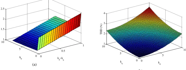
Fig. 6. VU-Factor versus changes in the odq-axis objective functions parameters.
VUF (%) =max(𝑣𝑎, 𝑣𝑏, 𝑣𝑐) − min(𝑣𝑎, 𝑣𝑏, 𝑣𝑐) 𝑉𝑎𝑣𝑔
× 100 (21) For each load scenario, the cost function parameters are changed sequentially. In the left side of Fig. 6, the parameter k0 is set to 7.5 and dq-axis gains (kdand kq) are changed
from 0.1 to 10. Herein, the THD rate is reduced when using
dq-axis gains smaller than 5 and can be minimized for gains around 1. In the right side of Fig. 6, the gain k0is changed
from 0.1 to 8 and dq-axis gains are taken equal and changed from 0.1 to 1. It can be seen that the THD evolution is more sensitive to the change dq-axis gains.
The evolution of VUF according to the cost function parameters is illustrated in Fig. 7. Thereafter, kdand kq are
taken equal and are linearly changed from 0 to 1 while ko is changed from 0.1 to 8. The VUF rate, as it can be appreciated, is further reduced for grater gains of k0. This
rate is minimized for k0 to 7.5 which satisfy VUF <2.2 %.
(b)
implementation. The chosen value of N for our practical implementation is equal to 6.
Fig. 7. Iteration number influence on the: THD (blue color), VUF (green color) and execution time (red color).
0 2 4 6 8 0 0.5 12 2.2 2.4 2.6 2.8 k0 k d=kq V U F ( % ) 0 5 10 15 20 25 1 1.5 2 2.5 3 3.5 4 4.5 T H D ( % ) Numbre of iteration 0 5 10 15 20 252 3 4 5 6 7 8 9 VU 0 2 4 6 8 10 12 14 16 18 E xe cut ion ti m e( us )
Fig. 5. Influence of the cost function odq-axis parameters on the voltage THD evolution: (a) ko gain influence when gains kd and kq are set equal, (b) kd and kq gains influence when ko is set to 10.
0 2 4 6 8 10
linear loads Non-linear loads
VU
F%
Proposed controller (Closed-loop) PI controller Flatness (Open-loop) 0 1 2 3 4 5
Linear loads Non-linear loads
TH
D
%
Proposed controller (Closed-loop) PI controller
Flatness (Open-loop) In summary, dq-axis gains (kd and kq) values are related to
the voltage quality and properly selected gain allows reducing the THD rate. Gain k0 acts on the voltage symmetry and allows reducing VUF rate. Notice that the iteration number is set to 6 in this test.
To illustrate the influence of the GW calculation burden on the effectiveness of the proposed tracking controller, the iteration number (N) is changed sequentially and several simulation tests under loading scenario are done. Fig. 7 groups the results obtained from the corresponding THD rate, the VUF rate and the calculation time. As it can be appreciated, the iteration number is a key parameter to satisfy the control effectiveness. Indeed, the obtained results show that iteration number 6 allows obtaining satisfactory control performance: i.e reduced THD and VUF rates with a minimized time calculation regarding real-time
A. Performance illustration
To underline the performance of the proposed controller, comparison tests with open-loop control based model and a conventional PI control method [43] are proposed. The open loop control is based on the flatness model where ÿ is set to zero in Fig. 3. The scheme principle of the conventional PI control is shown in Fig. 8.
+ vd vq d q0 /a b c P W M -v0 ref ref ref PI PI PI + -+ -ref v0 v0 vdref vd vqref vq + -iq + -id + -PI PI PI i0
Fig. 8. Block diagram of a conventional PI based FL-VSI control[45].
The PI parameters are selected by the use of pole placement method where the outer loop parameters kpv=5.33x10⁻³ kiv=1.42 and the inner loop kpi=120 et kii=316x103.
The compared three control strategies are firstly tested under linear load based on balanced resistive loads where Ra = Rb = Rc = 15 Ω. The obtained RMS voltages are presented in Fig. 9). As it can be appreciated, the open-loop control can be sufficient under ideal working conditions (balanced linear load where all parameters are known). Notice that the THD are equal to 2.1 for the open-loop, PI and proposed FBC-GWC controllers respectively. The compared controllers robustness is evaluated under unbalanced nonlinear loading conditions. The loads consist of single-phase diode rectifiers that cause zero sequence distortion at the odd triplen harmonics. For instance, load current phase a cause 2% of 3rd harmonic and 5% of 9th harmonic. The open-loop model is no longer sufficient and the use of closed-loop controller is necessary to handle the unbalance and harmonic issues. In
(a)
(b)
(c)
Fig.9. Obtained output voltage RMS and THD rate with open-loop, PI controller and closed-loop under balanced linear load and unbalanced nonlinear loads: (a) output voltage RMS (b) output voltage THD (c) output voltage
this way the use of a conventional PI controller and the proposed controller allow to significantly improve the power quality of the output voltage. The computed VUF values that correspond to open-loop, PI and proposed controller are 9.3%, 4.8% and 2.3% respectively, the correspondents VUF are reported in Fig 9c. The voltage THD of phase “a” are 4.6%, 2.6% and 1.3%, respectively; the correspondents THD rates are reported in Fig 9b.
The proposed control scheme achieves the lowest VUF and voltage THD values, which corresponds to better power quality.
To evaluate the effect of input voltage variation on the voltage regulation, the DC bus is changed from 400 to 600 V at t= 0.05s where the output RMS voltage reference is kept constant. As it can be appreciated, the AC voltage is not influenced by the DC bus voltage. The only condition is related to the controllability limit where the DC voltage level must be sufficient. The limit of DC bus voltage can be estimated as follow [46]: Vdc≥ VRMS2√2/(√3 m). For a
modulation index m = 0.5 , the minimal DC bus voltage to ensure controllability is around 360 V. Therefore, a DC bus voltage of 400 V is considered in this work.
Fig.10. Obtained output voltage RMS under input voltage variation
IV.EXPERIMENTALVERIFICATION
In order to validate the proposed control strategy, experiments are carried out. The control algorithm is implemented in a dSPACE (Micro-Auto-Box rapid
Zoom Zoom
v
bnv
cnv
anv
anv
bnv
cni
Lbi
Lci
Lai
Lai
Lbi
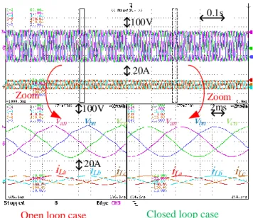
Lc 100V 0.1s 20A 2ms 100V 20AFig. 11. Experimental results: load voltages and currents during steady state with balanced resistive load before and
after activating the proposed control
prototyping platform). Different tests under different loading scenarios are performed to highlight the performance of the FB-GWC.
Fig.11. shows the steady state response of the load voltages and currents and their respective zooms under balanced resistive load before (open loop) and after activating the proposed control approach. The balanced resistive loads are set to Ra= Rb= Rc=15 Ω.When the proposed control is enabled the load voltage waveforms become purely sinusoidal and the voltage THD decreased from 8% (open loop) to 0.8%.
Fig.12. shows the steady state response of the load voltages and currents and their respective zooms under unbalanced resistive load before (open loop) and after activating the proposed control approach. The considered unbalanced resistive loads are set as Ra=∞ Ω and Rb= Rc=15 Ω. It can be noticed that the load voltage are balanced when the proposed control is applied and the measured voltage THD is decreased from 8.5% (open loop) to 1.1%.
In case of single phase load (Ra= Rb =∞ Ω and Rc=15 Ω), Fig. 13 illustrates the load voltages and currents responses and their respective zooms before (open loop) and after activating the proposed control approach. The load voltages are balanced. The noted voltage THD with the proposed control is about 1 %.
Zoom Zoom
v
bnv
cnv
anv
anv
bnv
cni
Lbi
Lci
Lai
Lai
Lbi
Lc 100V 0.1s 20A 2ms 100v 20AFig. 12. Experimental results: load voltages and currents during steady state with unbalanced resistive loads (Ra=∞Ω
and Rb= Rc=15Ω)before and after activating the proposed control. Zoom Zoom
v
bnv
cnv
anv
anv
bnv
cni
Lbi
Lci
Lai
Lai
Lbi
Lc 100v 0.1s 20A 2ms 100v 20AFig. 13. Experimental results: load voltages and currents during steady state with unbalanced resistive loads (Ra= Rb =∞Ω and Rc=15Ω)before and after activating the proposed
control.
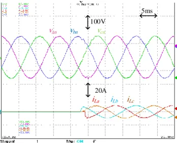
Fig.14. shows the output voltages and currents during a 0%- to-100% step of a balanced resistive load. The transient response lasted for only 3 ms. As clearly illustrated, the control showed good stability with no oscillatory behavior. Fig.15. shows the output voltages and currents during a single phase load and after balanced three-phase load. The transient response lasted for only 1 ms. Moreover, the pure sinusoidal voltage and current waves represent less voltage and current harmonics
v
bnv
cnv
ani
Lbi
Lci
La 100V 5ms 20AFig.14. Transient of 0%–100% balanced resistive load.
v
bnv
cnv
ani
Lbi
Lci
La 100v 5ms 20AFig. 15. Transient of single phase load to balanced resistive load.
To investigate the proposed approach performance in critical working conditions, a scenario of nonlinear unbalanced loads is considered. The considered unbalanced nonlinear loads are shown in Fig .16. The loads parameters are: phase a (Ra=80 Ω , Ca=1100 µF), phase b (Rb=20 Ω , Cb=500 µF) and phase c (Rc=100 Ω , Lc=30 mH). a b Ra Ca Rc Lc Rb Cb c
Fig. 16. Topology of the tested unbalanced nonlinear loads.
For this loading scenario, the output load voltages, and load currents waveforms before (open loop) and after activating the proposed control are shown in Fig.17. The voltage THD values are reported in Table 2. This test shows that the proposed control scheme allow keeping the load voltages balanced with a reasonable voltage THD.
Referring to these results, it can be concluded that in steady state with balanced or unbalanced linear or nonlinear loading conditions, the use of the proposed control approach allows to keep the load voltages balanced with a voltage THD less than 2%. Zoom Zoom
v
bnv
cnv
anv
anv
bnv
cni
Lbi
Lci
Lai
Lai
Lbi
Lc 100v 0.1s 20A 2ms 100v 20AFig.17. Experimental results: load voltages and currents during steady state with unbalanced nonlinear loads before and after
activating the proposed control. TABLE 2
LOAD VOLTAGE THD FOR A THREE-PHASE
THD (%) Phase a Phase b Phase c Open Loop 8.8 10.8 10.1 Flatness Based GW Control 1.8 1.7 2
The analysis of the reported THD values regarding robustness against parameter variations proves that the proposed control allows obtaining a lower voltage THD value.
The evolution of the (THD) versus the variations in Lf with balanced ((Ra= Rb= Rc=15 Ω) and unbalanced (Ra=∞ and Rb= Rc=15 Ω) loading conditions. the load voltage THD values of the proposed approach for different L values (1 mH, 2 mH, 3 mH) are shown in In Fig 18.
Fig.18. Load voltage THD versus value of Inductor (Lf)
under balanced linear load (blue color) and unbalanced nonlinear loads (red color).
Fig.19. Load voltage THD versus value of capacitor (Cf)
under balanced linear load (blue color) and unbalanced nonlinear loads (red color).
In Fig 19, the evolution of the load voltage THD versus the variations in Cf with balanced ((Ra= Rb= Rc=15 Ω, blue curve) and unbalanced (Ra=∞ and Rb= Rc=15 Ω, red curve) loading conditions, when the parameter L is set to 1 and Cf is changed from 20 uF to 100 uF. It can be seen that the THD evolution is less sensitive to the Cf superior 40 uF. The analysis of the fig 18 and 19 shows that the variations in Cf have more impact on the load voltages than the Lf variations.
V. Conclusion
In this paper a voltage control strategy based on a Flatness theory with a Grey Wolf tracking control (FB-GWC) has been proposed for a four-leg inverter with an output LC filter for use in Three-Phase Four-Leg Voltage Source Inverters. The proposed FB-GWC control scheme can be split into two subsystems: the flat model of the system and the GW tracking controller. The differentially flat model of the FL-VSI allows calculating the control inputs as differential functions of the flat outputs and their derivatives. The GW tracking controller provide the correction control effort used by the differentially flat model in such a way to ensure the desired trajectory
0.5 1 1.5 2 2.5 3 0 0.5 1 1.5 2 2.5 3 L (mH) T H D ( % ) 0 20 40 60 80 100 0 1 2 3 4 5 6 C f (uF) T H D ( % )
tracking tasks especially in case of the presence of heavy nonlinearity or unbalanced loads.
The provided experimental results demonstrated that the proposed control approach allows keeping the load voltage balanced with a reasonable voltage THD rate when the system is subject to disturbances like nonlinear and unbalanced loads.
REFERENCES
[1]Kabiri, R., Holmes, D. G., & McGrath, B. P. (2015). Control of active and reactive power ripple to mitigate unbalanced grid voltages. IEEE Trans. Ind. Appl, vol. 52, no.2, pp. 1660-1668, 2015.
[2]Iyer, S. V., Belur, M. N., & Chandorkar, M. C. (2010). A generalized computational method to determine stability of a multi-inverter microgrid. IEEE Trans on Power Electron, vol. 25, no. 9, pp. 2420-2432, 2010. [3] F. Blaabjerg; Y. Yang; D. Yang and X. Wang “ Distributed Power Generation Systems and Protection” IEEE Journals & Magazines, Vol 105, pp. 1311 - 1331, 2017.
[4]Iyer, S. V., Belur, M. N., & Chandorkar, M. C. Analysis and mitigation of voltage offsets in multi-inverter microgrids. IEEE Trans. on Energy Conversion, vol. 26, no.1, pp. 354-363, 2010.
[5] W. Wu, Y. Liu, Y. He, H. Shu-Hung Chung, M. Liserre and F. Blaabjerg, “Damping Methods For Resonances Caused By Lcl-Filter-Based Current-Controlled Grid-Tied Power Inverters: An Overview,” IEEE Trans. Ind. Electron, vol. 64, no. 9, pp. 7402 - 7413, 2017.
[6] IEEE standard 519-1992, ” IEEE Recommended Practice and Requirement for Harmonic Control in Electric Power Systems” Institute of Electrical and Electronics, Inc 1993.
[7] IEEE standard 1547-2003 “IEEE standard for interconnecting distributed resources with electric power systems”, Institute of Electrical and Electronics, Inc 2014.
[8] M. Zhang, D. J. Atkinson, B. Ji, M. Armstrong, and M. Ma, “A near-state three-dimensional space vector modulation for a three-phase four-leg voltage source inverter,” IEEE Trans. Power Electron., vol. 29, no. 11, pp. 5715– 5726, 2014
[9] M. Pichan, H. Rastegar, and M. Monfared, “Deadbeat control of the stand-alone four-leg inverter considering the effect of the neutral line inductor,” IEEE Trans. Ind. Electron., vol. 0046, no. c, 2016.
[10] S. Bifaretti, A. Lidozzi, L. Solero, and F. Crescimbini, “Modulation with Sinusoidal Third-Harmonic Injection for Active Split DC-Bus Four-Leg Inverters,” IEEE Trans. Power Electron., vol. 31, no. 9, pp. 6226–6236, 2016 [11] A. Lidozzi, C. Ji, L. Solero, F. Crescimbini, and P. Zanchetta, “Load-Adaptive Zero-Phase-Shift Direct Repetitive Control for Stand-Alone Four-Leg VSI,” IEEE Trans. Ind. Appl., vol. 52, no. 6, pp. 4899–4908, 2016 [12] I. Vechiu, O. Curea, and H. Camblong, “Transient operation of a four-leg inverter for autonomous applications with unbalanced load,” IEEE Trans. Power Electron., vol. 25, no. 2, pp. 399–407, 2010.
[13] X. Zhou, F. Tang, P. C. Loh, X. Jin, and W. Cao, “Four-Leg Converters with Improved Common Current Sharing and Selective Voltage-Quality Enhancement for Islanded Microgrids,” IEEE Trans. Power Deliv., vol. 31, no. 2, pp. 522–531, 2016
[14] A. Houari, A. Djerioui, A. Saim, M. Ait-Ahmed, M. Machmoum " Improved Control Strategy for Power Quality Enhancement in Standalone Systems Based on Four-Leg Voltage Source Inverters" IET Power Electronics, Vol. pp, No. pp, 2017.
[15] B. Ufnalski, A. Kaszewski, and L. M. Grzesiak, “Particle swarm optimization of the multioscillatory LQR for a three-phase four-wire voltage-source inverter with an LC output filter,” IEEE Trans. Ind. Electron, vol. 62, no. 1, pp. 484–493, 2015.
[16] Vyawahare, D., & Chandorkar, M. (2016). Design and analysis of stand-alone 4-wire, 4-leg inverter microgrid with unbalanced loads. EPE Journal, 26(2),. , vol. 26, no. 2, pp. 71-834, 2016.
[17] C. Burgos-Mellado, C. Hernández-Carimán, R. Cárdenas, D. Sáez, M. Sumner, A. Costabeber and H. Morales "Experimental Evaluation of a
CPT-Based Four-Leg Active Power Compensator for Distributed Generation" IEEE Journal Of Emerging And Selected Topics In Power Electron, Vol. 5, N. 2, pp 747 - 759, 2017
[18] H. Golwala and R. Chudamani "New Three Dimensional Space Vector based Switching Signal Generation Technique without Null Vectors and with Reduced Switching Losses for a Grid-Connected Four-leg Inverter" IEEE Trans. Power Electron., vol. 31, no. 2, pp. 1026-1035, 2016.
[19] M. Pichan and H. Rastegar "Sliding-Mode Control of Four-Leg Inverter With Fixed Switching Frequency for Uninterruptible Power Supply Applications" IEEE Trans. Ind. Electron, vol. 64, no. 8, pp. 6805-6814, 2017.
[20] A. Chebabhi, M. K. Fellah, A. Kessal, and M. F. Benkhoris, “A new balancing three level three dimensional space vector modulation strategy for three level neutral point clamped four leg inverter based shunt active power filter controlling by nonlinear back stepping controllers,” ISA Trans., vol. 63, pp. 328–342, 2016.
[21] M. Bouzidi, A. Benaissa, and S. Barkat, “Hybrid direct power/current control using feedback linearization of three-level four-leg voltage source shunt active power filter,” Int. J. Electr. Power Energy Syst., vol. 61, pp. 629–646, 2014.
[22]Sawant, R. R., & Chandorkar, M. C. (2009). A multifunctional four-leg grid-connected compensator. IEEE Trans. Ind. Appl, vol. 45, no. 1, pp. 249-259, 2009.
[23] R. Lliuyacca, J. Mauricioa, A. Gomez-Exposito, M. Savaghebi and J. Guerrero. “Grid-forming VSC control in four-wire systems with unbalanced nonlinear loads" Elect Power Sys Research, vol 152, pp 249- 256. 2017. [24] S.R. Naidu ; D.A. Fernandes “Dynamic voltage restorer based on a four-leg voltage source converter” IET Generation, Transmission & Distribution vol 3 N 5, pp 437- 447. 2009.
[25] E. Demirkutlu ; A. Hava A Scalar Resonant-Filter-Bank-Based Output-Voltage Control Method and a Scalar Minimum-Switching-Loss Discontinuous PWM Method for the Four-Leg-Inverter-Based Three-Phase Four-Wire Power Supply" IEEE Trans. Ind. Appl., vol. 45, no. 3, pp. 982 - 991, 2009.
[26] Patel, D. C., Sawant, R. R., & Chandorkar, M. C. (2009). Three-dimensional flux vector modulation of four-leg sine-wave output inverters. IEEE Trans. Ind. Electron., vol. 57, no. 4, pp. 1261-1269, 2009.
[27] PC Loh, MJ Newman, DN Zmood, DG Holmes,A comparative analysis of multiloop voltage regulation strategies for single and three-phase UPS systems. IEEE Trans. Ind. Electron., vol. 18, no. 5, pp. 1176-1185,2003. [28] PC Loh, DG Holmes. Analysis of multiloop control strategies for LC/CL/LCL-filtered voltage-source and current-source inverters. IEEE Transactions on Industry Applications, IEEE Trans. Ind. Appl., vol. 41, no. 2, pp. 644-654, 2005.
[29] D. E. Kim and D. C. Lee, “Feedback linearization control of three-phase UPS inverter systems,” IEEE Trans. Ind. Electron., vol. 57, no. 3, pp. 963– 968, 2010.
[30] M. S. Badra, S. Barkat, M. Bouzidi "Backstepping control of three-phase three-level four-leg shunt active power filter Journal of Fundamental and Applied Sciences Vol 9, No 1, 2017
[31]Rivera, M., Yaramasu, V., Llor, A., Rodriguez, J., Wu, B., & Fadel, M.. Digital predictive current control of a three-phase four-leg inverter. IEEE Trans. Ind. Electron., vol. 60, no. 11, pp. 4903-4912, 2012.
[32] V. Yaramasu, M. Rivera, M. Narimani, B. Wu, and J. Rodriguez, “Model predictive approach for a simple and effective load voltage control of four-leg inverter with an output LC filter,” IEEE Trans. Ind. Electron., vol. 61, no. 10, pp. 5259–5270, 2014.
[33] S. Bayhan, M. Trabelsi, H. Abu-Rub, and M. Malinowski, “Finite Control Set Model Predictive Control for a Quasi-Z-Source Four-Leg Inverter Under Unbalanced Load Condition,” IEEE Trans. Ind. Electron., vol. 46, no. c, pp. 1–1, 2016.
[34] A. Houari ; H. Renaudineau ; J. Martin ; S. Pierfederici ; F. Meibody-Tabar " Flatness-Based Control of Three-Phase Inverter With OutputLC Filter" IEEE Trans. Ind. Electron., vol. 59, no. 7, pp. 2890–2897, 2012.
[35] A. Shahin , H. Moussa , I. Forrisi, J. Martin ; B. Nahid-Mobarakeh and S. Pierfederici "Reliability Improvement Approach Based on Flatness Control of Parallel-Connected Inverters" IEEE Trans. Power Electron., vol. 32, no. 1, pp. 681 - 692, 2017.
Nahid-Mobarakeh ; S. Pierfederici "Flatness-based control method: A review of its applications to power systems" 7th Power Electronics and Drive Systems Technologies Conference (PEDSTC), 16-18 Feb. 2016
[37] A. Djerioui, A. Houari, M. Ait-Ahmed, M.F Benkhoris, A. Chouder and M. Machmoum " Grey Wolf based control for speed ripple reduction at low speed operation of PMSM drives" ISA Trans., vol. PP, pp. 1–8, 2018. [38] Kim J-H, Sul S-K. A carrier-based PWM method for three-phase four-leg voltage source converters. IEEE Trans Power Electron 2004;19(1):66–75. [39] S. Mirjalili, S. M. Mirjalili, and A. Lewis, “Grey Wolf Optimizer,” Adv. Eng. Softw., vol. 69, pp. 46–61, 2014.
[40] R.E. Precup, R.-C. David and E.M. Petriu, " Grey wolf optimizer algorithm-based tuning offuzzy control systems with reduced parametric sensitivity. IEEE Transactions on Industrial Electronics 64, 1,. 527–534.2017 [41] A Djerioui, A Houari, S Zeghlache, A Saim, MF Benkhoris, T Mesbahi, M. Machmoum “Energy management strategy of Supercapacitor/Fuel Cell energy storage devices for vehicle applications,” International Journal of Hydrogen Energy, vol. 44, pp. 23416-23428, 2019. [42] S. Sharma, S. Bhattacharjee, and A. Bhattacharya, “Grey wolf optimisation for optimal sizing of battery energy storage device to minimise operation cost of microgrid,” IET Gener. Transm. Distrib., vol. 10, no. 3, pp. 625–637, 2016.
[43] S. Bella, A. Djcrioui, A. Houari, A. Chouder, M. Machmoum, M-F. Benkhoris, K. Ghedamsi, “Model-Free Controller for Suppressing Circulating Currents in Parallel-Connected Inverters,“ in Proc. 2018 IEEE Ind. Appl. Soc. Ann. Meeting, Portland, OR, USA, pp. 1-6.
[44] Palanisamy Ramasamy and Vijayakumar Krishnasamy "A 3D-Space Vector Modulation Algorithm for Three Phase Four Wire Neutral Point Clamped Inverter Systems as Power Quality Compensator" Energies, Vol 10, pp. 1792, 2017
[45] Nayeem Ahmed Ninad, Luiz Lopes "Per-phase vector control strategy for a four-leg voltage source inverter operating with highly unbalanced loads in stand-alone hybrid systems" Electr. Power Energy Systems, vol. 55, pp. 449–459, Feb. 2014
[46] M.Rezkallah, S.Sharma, A.Chandra, B.Singh and D.R. Rousse " Lyapunov Function and Sliding Mode Control Approach for the Solar-PV Grid Interface System'' IEEE Trans. Ind. Electron., vol. 64, no. 1, pp. 785 - 795, 2017
Ali DJERIOUI was born in M'sila, Algeria, in 1986.In 2009,he received the engineering degree in electrical engineering from the University of M'sila, Algeria. In 2011,he was graduated M.Sc. degree in electrical engineering from the Polytechnic Military Academy in Algiers, Algeria. I obtained in 2016 the doctorate degree in Electronic Instrumentation systems from University of Science and Technology Houari Boumediene, Algiers, Algeria and the “HDR” in MAY 2018. He is currently assistant professor in the university of mohamed boudiaf, M'sila, Algeria. His current research interests include power electronics, control, microgrids and power quality.
Azeddine HOUARI received the Engineer degree in 2008 from Bejaia University (Algeria) and a Ph.D. degree in 2012 from Lorraine University (France). Since 2014, he works as an assistant professor at Nantes University (France) and exercises his research activities with the Institut de Recherche en Énergie Électrique de Nantes Atlantique (IREENA). His current research deals with the power quality and the stability issues in stationary and embedded DC and AC micro-grids.
Abdelhakim SAIM was born in Batna, Algeria, on February 02, 1990. He received the B.S. and the M.S. degrees in electronics and control engineering both from Blida University, Algeria, in 2010 and 2012, respectively, and the Ph.D. degree in control engineering from Tizi-Ouzou University, Algeria, in 2017. Since 2017, he has been an Assistant Professor with the Department of Control and Instrumen-tation, University of Sciences and Technology Houari Boumediene, Algiers, Algeria. His current research deals with the power quality and stability of microgrids.
Mourad AIT-AHMED was born in Djelfa, Algeria, on June 21, 1965. He received the Engineering degree in 1988 from the ENITA, Algeria. In 1993 he obtained his PhD degree in Robotic at LAAS-CNRS, Toulouse and the “HDR” in November 2017. From 1993 he is at the Departement of Electrical Engineering, Polytech Nantes, France, where he is an Associate Professor in automatic control and he exercises his research activities with IREENA. His main research interests are in the fields of modeling and control of multi-phase electrical machines, embedded electrical networks and microgrids.
Serge PIERFEDERICI received Engineer degree in electrical engineering at ENSEM, Nancy, France in 1994 and the Ph.D. degree from INP Lorraine, France, in 1998. Since 2009, he has been engaged as Professor at INPL. His research activities deals with the stability study of distributed power system and the control of multi sources, multi load systems. Mohamed Fouad BENKHORIS was born in Bou-sâada, Algeria, on September 17, 1963. He has studied at Ecole Nationale Polytechnique d’Alger , Algeria, and received the Engineer degree in electrical engineering (1986). In 1991 he obtained his PHD degree in electrical engineering at INP Lorraine (France) and the “HDR” in March 2004. Since 2006 he is Professor at PolytechNantes, France. Currently he is the deputy director of PolytechNantes . He makes research activities at the laboratrory IREENA Saint Nazaire. His fields of interest are: control of electrical drives and especially multi phase drive, multi-converters systems embarked network
and renewable energy.
Mohamed MACHMOUM was born in
Casablanca, Morocco, on November 29, 1961. He received the Diplo. Engineering Degree in 1984 from the “Institut Supérieur Industriel” of Liège, Belgium, the Ph.D. degree from the “Institut National Polytechnique of Lorraine (INPL)”, France, in 1989, all in electrical engineering. In 1991, he joined “l’Ecole Polytechnique de l’Université de Nantes” as Assistant Professor. Since September 2005 he is a Professor at the same Engineering School. He is actually the head of IREENA laboratory, University of Nantes. His main area of interest includes power electronics, power quality, tidal energy conversion systems and microgrids.
Malek Ghanes received the M.Sc. and Ph.D. degrees in applied automation and informatics from the IRCCyN, Ecole Centrale Nantes, France, in 2002 and 2005, respectively.From September 2006 to April 2016, he was with the ECS-Lab, Quartz, École Nationale Supérieure de l’Électronique et de ses Applications, Cergy, France, where he was an Associate Professor and the Head of the Department of Automation and Electrical Engineering. Since May 2016, he has been to a Full Professor at IRCCyN-ECN. His research interests include observation and control of nonlinear systems. He is currently a Research Chair on Electrics Vehicles between Renault and IRCCyN-ECN.
![Fig .2. Carrier based PWM technique [38]](https://thumb-eu.123doks.com/thumbv2/123doknet/12509178.340981/5.918.80.448.104.331/fig-carrier-based-pwm-technique.webp)
![Fig. 8. Block diagram of a conventional PI based FL-VSI control[45].](https://thumb-eu.123doks.com/thumbv2/123doknet/12509178.340981/9.918.471.844.111.908/fig-block-diagram-conventional-pi-based-vsi-control.webp)