HAL Id: hal-00960609
https://hal.inria.fr/hal-00960609
Submitted on 18 Mar 2014
HAL is a multi-disciplinary open access
archive for the deposit and dissemination of
sci-entific research documents, whether they are
pub-lished or not. The documents may come from
teaching and research institutions in France or
abroad, or from public or private research centers.
L’archive ouverte pluridisciplinaire HAL, est
destinée au dépôt et à la diffusion de documents
scientifiques de niveau recherche, publiés ou non,
émanant des établissements d’enseignement et de
recherche français ou étrangers, des laboratoires
publics ou privés.
RDF Analytics: Lenses over Semantic Graphs
Dario Colazzo, François Goasdoué, Ioana Manolescu, Alexandra Roatis
To cite this version:
Dario Colazzo, François Goasdoué, Ioana Manolescu, Alexandra Roatis. RDF Analytics: Lenses over
Semantic Graphs. 23rd International World Wide Web Conference, Apr 2014, Seoul, South Korea.
�10.1145/2566486.2567982�. �hal-00960609�
RDF Analytics: Lenses over Semantic Graphs
Dario Colazzo
U. Paris Dauphine & Inria, France
François Goasdoué
U. Rennes 1 & Inria, France
Ioana Manolescu
Inria & U. Paris-Sud, France
Alexandra Roati¸s
U. Paris-Sud & Inria, France
ABSTRACT
The development of Semantic Web (RDF) brings new requirements for data analytics tools and methods, going beyond querying to semantics-rich analytics through warehouse-style tools. In this work, we fully redesign, from the bottom up, core data analytics concepts and tools in the context of RDF data, leading to the first complete formal framework for warehouse-style RDF analytics. Notably, we define i) analytical schemas tailored to heterogeneous, semantics-rich RDF graph, ii) analytical queries which (beyond relational cubes) allow flexible querying of the data and the schema as well as powerful aggregation and iii) OLAP-style operations. Experiments on a fully-implemented platform demonstrate the practical interest of our approach.
Categories and Subject Descriptors
H.2.1 [Database Management]: Logical Design;
H.2.7 [Database Management]: Database Administration —Data warehouse and repository
Keywords
RDF; data warehouse; OLAP
1.
INTRODUCTION
The development of Semantic Web data represented within W3C’s Resource Description Framework [33] (or RDF, in short), and the associated standardization of the SPARQL query language now at v1.1 [35] has lead to the emergence of many systems capable of storing, querying, and updating RDF, such as OWLIM [38], RDF-3X [28], Virtuoso [15] etc. However, as more and more RDF datasets are made avail-able, in particular Linked Open Data, application require-ments also evolve. In the following scenario, we identify by (i)-(v) a set of application needs, for further reference.
Alice is a software engineer working for an IT company re-sponsible of developing user applications based on open (RDF) data from the region of Grenoble. From a dataset describing the region’s restaurants, she must build a click-able map showing for each district of the region, “the number of restaurants and their average rating per type of cuisine”.
c
2014 International World Wide Web Conference Committee.
This is an electronic version of an article published in WWW’14, April 7–11, 2014, Seoul, Korea. http://dx.doi.org/10.1145/2566486.2567982.
The data is (i) heterogeneous, as information, such as the menu, opening hours or closing days, is available for some restaurants, but not for others. Fortunately, Alice studied data warehousing [22]. She thus designs a relational data warehouse (RDW, in short), writes some SPARQL queries to extract tabular data from the restaurant dataset (filled with nulls when data is missing), loads them in the RDW and builds the application using standard RDW tools.
The client is satisfied, and soon Alice is given two more datasets, on shops and museums; she is asked to (ii) merge them in the application already developed. Alice has a hard time: she had designed a classical star schema [23], cen-tered on restaurants, which cannot accommodate shops. She builds a second RDW for shops and a third for museums.
The application goes online and soon bugs are noticed. When users search for landmarks in an area, they don’t find anything, although there are multiple museums. Alice knows this happens because (iii) the RDW does not capture the fact that a museum is a landmark. With a small redesign of the RDW, Alice corrects this, but she is left with a nagging feeling that there may be many other relationships present in the RDF which she missed in her RDW. Further, the client wants the application to find (iv) the relationships between the region and famous people related to it, e.g., Stendhal was born in Grenoble. In Alice’s RDWs, relationships be-tween entities are part of the schema and statically fixed at RDW design time. In contrast, useful open datasets such as DBpedia [1], which could be easily linked with the RDF restaurant dataset, may involve many relationships between two classes, e.g., bornIn, gotMarriedIn, livedIn etc.
Finally, Alice is required to support (v) a new type of aggregation: for each landmark, show how many restaurants are nearby. This is impossible in Alice’s RDW designs of a separate star schema for each of restaurants, shops and landmarks, as both restaurants and landmarks are central entities and Alice cannot use one as a measure for the other. Alice’s needs in setting up the application can be summa-rized as follows: (i) support of heterogeneous data; (ii) multi-ple central concepts, e.g., restaurants and landmarks above; (iii) support for RDF semantics when querying the ware-house, (iv) the possibility to query the relationships between entities (similar to querying the schema), (v) flexible choice of aggregation dimensions.
In this work, we perform a full redesign, from the bottom up, of the core data analytics concepts and tools, leading to a complete formal framework for warehouse-style analyt-ics on RDF data; in particular, our framework is especially
suited to heterogeneous, semantic-rich corpora of Linked Open Data. Our contributions are:
• We devise a full-RDF warehousing approach, where the base data and the warehouse extent are RDF graphs. This answers to the needs (i), (iii) and (iv) above. • We introduce RDF Analytical Schemas (AnS), which
are graphs of classes and properties themselves, having nodes (classes) connected by edges (properties) with no single central concept (node). This contrasts with the typical RDW star or snowflake schemas, and caters to requirement (ii) above. The core idea behind many-node analytical schemas is to define each many-node (resp. edge) by an independent query over the base data. • We define Analytical Queries (AnQ) over our
decen-tralized analytical schemas. Such queries are highly flexible in the choice of measures and classifiers (requirement (v)), while supporting all the classical analytical cubes and operations (slice, dice etc.). • We fully implemented our approach in an operational
prototype and empirically demonstrate its interest and performance.
The remainder of this paper is organized as follows. We recall RDF data and queries in Sections 2 and 3. Section 4 presents our analytical schemas and queries, and Section 5 studies efficient query evaluation methods. Section 6 intro-duces typical analytical operations (slice, dice etc.) on our RDF analytical cubes. We present our experimental evalu-ation in Section 7, discuss related work, and then conclude.
2.
RDF GRAPHS
An RDF graph (or graph, in short) is a set of triples of the form s p o. A triple states that its subject s has the property p, and the value of that property is the object o.
We consider only well-formed RDF triples, as per the RDF specification [33], using uniform resource identifiers (URIs), typed or un-typed literals (constants) and blank nodes (un-known URIs or literals).
Notation. We use s, p, o in triples as placeholders. Literals are shown as strings between quotes, e.g., “string”. Finally, the set of values – URIs (U ), blank nodes (B), literals (L) – of an RDF graph G is denoted Val(G).
Figure 1 (top) shows how to use triples to describe re-sources, that is, to express class (unary relation) and prop-erty (binary relation) assertions. The RDF standard [33] provides a set of built-in classes and properties, as part of the rdf: and rdfs: pre-defined namespaces. We use these names-paces exactly for these classes and properties, e.g., rdf:type specifies the class(es) to which a resource belongs.
Below, we formalize the representation of an RDF graph using graph notations. We use f|dto denote the restriction of a function f to its sub-domain d. Our formalization follows the RDF standard [33].
Definition 1. (Graph notation of an RDF graph) An RDF graph is a labeled directed graphG= hN , E, λiwith: • N is the set of nodes, let N0 denote the nodes in N
having no outgoing edge, and let N>0= N \ N0; • E ⊆ N>0× N is the set of directed edges;
• λ : N ∪ E → U ∪ B ∪ L is a labeling function such that λ|N is injective, with λ|N0 : N0→ U ∪ B ∪ L and
λ|N>0 : N>0→ U ∪ B, and λ|E : E → U .
Assertion Triple Relational notation
Class srdf:type o o(s)
Property s p o p(s, o)
Constraint Triple OWA interpretation
Subclass srdfs:subClassOf o s⊆ o
Subproperty srdfs:subPropertyOf o s⊆ o
Domain typing srdfs:domain o Πdomain(s) ⊆ o
Range typing srdfs:range o Πrange(s) ⊆ o
Figure 1: RDF (top) & RDFS (bottom) statements.
G=
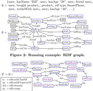
{user1hasName “Bill”, user1hasAge “28”, user1friend user3, user1bought product1, product1rdf:type SmartPhone, user1worksWith user2, user2hasAge “40”, . . .}
G= user1 user2 worksWith user3 friend William hasName Bill hasName 28 hasAge Madrid inCity Student rdf:type product1 bought brand1 hasBrand 400 hasPrice SmartPhone rdf:type rating1 gave on good deal hasValue Rating rdf:type post1 post2 post3 post4 wrote wrote wrote wrote blog1 blog2 inBlog inBlog inBlog inBlog 40 hasAge 35 hasAge NY inCity
Figure 2: Running example: RDF graph.
G′= G ∪ SmartPhone Phone Notebook Product sc sc sc Person Student sc wrote dm bought dm rg hasBrand Brand dm rg inBlog Message Blog dm rg xsd:int hasAge rg hasPrice rg knows rg dm worksWith sp friend sp sc = rdfs:subClassOf sp = rdfs:subPropertyOf dm = rdfs:domain rg = rdfs:range
Figure 3: Running example: RDF Schema triples. Example 1. (RDF Graph) We consider an RDF graph comprising information about users and products. Figure 2 shows some of the triples (top) and depicts the whole dataset using its graph notation (bottom). The RDF graph features a resource user1 whose name is “Bill” and whose age is “28”. Bill works with user2and is a friend of user3. He is an active contributor to two blogs, one shared with his co-worker user2. Bill also bought a SmartPhone and rated it online etc.
A valuable feature of RDF is RDF Schema (RDFS) that allows enhancing the descriptions in RDF graphs. RDFS triples declare semantic constraints between the classes and the properties used in those graphs. Figure 1 (bottom) shows the allowed constraints and how to express them; do-main and range denote respectively the first and second at-tribute of every property. The RDFS constraints (Figure 1) are interpreted under the open-world assumption (OWA) [7]. For instance, given two relations R1, R2, the OWA interpre-tation of the constraint R1 ⊆ R2 is: any tuple t in the re-lation R1 is considered as being also in the relation R2 (the inclusion constraint propagates t to R2).
Example 2. (RDF Schema) Consider next to the graph G from Figure 2, the schema depicted in Figure 3. This schema expresses semantic (or ontological) constraints like a Phone is a Product, a SmartPhone is a Phone, a Student is a Person, the domain and range of knows is Person, that working with someone is one way of knowing her etc. RDF entailment. Our discussion on constraint interpre-tation above illustrated an important RDF feature: implicit
triples, considered part of the RDF graph even though they are not explicitly present in it. An example is product1 rdf:type Phone, which is implicit in the graph G′ of Fig-ure 3. W3C names RDF entailment the mechanism through which, based on a set of explicit triples and some entail-ment rules, implicit RDF triples are derived. We denote by ⊢i
RDF immediate entailment, i.e., the process of deriving new
triples through a single application of an entailment rule. More generally, a triple s p o is entailed by a graph G, de-noted G ⊢RDF s p o, if and only if there is a sequence of
applications of immediate entailment rules that leads from Gto s p o (where at each step of the entailment sequence, the triples previously entailed are also taken into account). Saturation. The immediate entailment rules allow defin-ing the finite saturation (a.k.a. closure) of an RDF graph G, which is the RDF graph G∞defined as the fix-point obtained by repeatedly applying ⊢i
RDF on G.
The saturation of an RDF graph is unique (up to blank node renaming), and does not contain implicit triples (they have all been made explicit by saturation). An obvious con-nection holds between the triples entailed by a graph G and its saturation: G ⊢RDFs p oif and only if s p o ∈ G∞.
RDF entailment is part of the RDF standard itself; in par-ticular, the answers of a query posed on G must take into ac-count all triples in G∞, since the semantics of an RDF graph is its saturation. In Sesame [39], Jena [37], OWLIM [38] etc., RDF entailment is supported through saturation.
3.
BGP QUERIES
We consider the well-known subset of SPARQL consist-ing of (unions of) basic graph pattern (BGP) queries, also known as SPARQL conjunctive queries. A BGP is a set of triple patterns, or triples in short. Each triple has a subject, property and object, some of which can be variables. Notation. In the following we will use the conjunctive query notation q(¯x):- t1, . . . , tα, where {t1, . . . , tα} is a BGP; the query head variables ¯x are called distinguished variables, and are a subset of the variables occurring in t1, . . . , tα; for boolean queries ¯x is empty. The head of q denoted head(q) is q(¯x), and the body of q denoted body(q) is t1, . . . , tα. We use x, y, and z (possibly with subscripts) to denote variables in queries. We denote by VarBl(q) the set of variables and blank nodes occurring in the query q.
BGP query graph. For our purposes, it is useful to view each triple atom in the body of a BGP query as a generalized RDF triple, where variables may appear in any of the sub-ject, predicate and object positions. This leads to a graph notation for BGP queries, which can be seen as a corre-sponding generalization of our RDF graph representation (Definition 1). For instance, the body of the query:
q(x, y, z):- x hasName y, x z product1 is represented by the graph:
x
y
hasName zproduct
1Query evaluation. Given a query q and an RDF graph G, the evaluation of q against G is:
q(G) = {¯xµ| µ : VarBl(q) → Val(G) is a total assignment such that tµ 1 ∈ G, t µ 2 ∈ G, . . . , t µ α∈ G}
where we denote by tµ the result of replacing every occur-rence of a variable or blank node e ∈ VarBl(q) in the triple t, by the value µ(e) ∈ Val(G).
Notice that evaluation treats the blank nodes in a query exactly as it treats non-distinguished variables [8]. Thus, in the sequel, without loss of generality, we consider queries where all blank nodes have been replaced by distinct (new) non-distinguished variable symbols.
Query answering. The evaluation of q against G uses only G’s explicit triples, thus may lead to an incomplete answer set. The (complete) answer set of q against G is obtained by the evaluation of q against G∞, denoted by q(G∞).
Example 3. (BGP Query Answering) The following query on G′ (Figure 3) asks for the names of those having bought a product related to Phone:
q(x) :- y1 hasName x, y1 bought y2, y2 y3 Phone Here, q(G′∞) = {h“Bill”i, h“William”i}.
The answer results from G′⊢RDF product1rdf:type Phone
and the assignments:
µ1= {y1→ user1, x → Bill, y2→ product1, y3→ rdf:type}and
µ2= {y1→ user1, x → William, y2→ product1, y3→ rdf:type}. Note that evaluating q against G′ leads to the incomplete (empty) answer set q(G′) = {hi}.
BGP queries for data analysis. Data analysis typically allows investigating particular sets of facts according to rel-evant criteria (a.k.a. dimensions) and measurable or count-able attributes (a.k.a. measures) [23]. In this work, rooted BGP queries play a central role as they are used to specify the set of facts to analyze, as well as the dimensions and the measures to be used (Section 4.2).
Definition 2. (Rooted Query) Let q be a BGP query, G = hN , E, λi its graph and n ∈ N a node whose label is a variable in q. The query q is rooted in n iff G is a con-nected graph and any other node n′ ∈ N is reachable from n following the directed edges in E.
Example 4. (Rooted Query) The query q described be-low is a rooted BGP query, with x1 as root node.
q(x1, x2, x3) :- x1 knows x2, x1 hasName y1, x1 wrote y2, y2 inBlog x3
The query’s graph representation below shows that every node is reachable from the root x1.
x
1x
2y
1y
2x
3 knows hasName wrote inBlogNext, we introduce the concept of join query, which joins BGP queries on their distinguished variables and projects out some of these variables. Join queries will be used when defining data warehouse analyses.
Definition 3. (Join Query) Let q1, . . . , qn be BGP queries whose non-distinguished variables are pairwise dis-joint. We say q(¯x):- q1(¯x1) ∧ · · · ∧ qn(¯xn), where ¯x ⊆ ¯x1∪ · · · ∪ ¯xn, is a join query q of q1, . . . , qn. The answer set to q(¯x) is defined to be that of the BGP query q✶:
q✶(¯x):- body(q
1(¯x1)), · · · , body(qn(¯xn))
In the above, q1, q2, . . . , qndo not share non-distinguished variables (variables not present in the query head). This assumption is made without loss of generality, as one can easily rename non-distinguished variables in q1, q2, . . . , qnin order to meet the condition. In the sequel, we assume such renaming has been applied in join queries.
Example 5. (Join Query) Consider the BGP queries q1, asking for the users having bought a product and their age, and q2, asking for users having posted in some blog:
q1(x1, x2) :- x1 bought y1, x1 hasAge x2 q2(x1, x3) :- x1 wrote y2, y2 inBlog x3
The join query q1,2(x1, x2) :- q1(x1, x2) ∧ q2(x1, x3) asks for the users and their ages, for all the users having posted in a blog and having bought a product, i.e.,
q✶
1,2(x1, x2) :- x1 bought y1, x1 hasAge x2, x1 wrote y2, y2 inBlog x3
Other join queries can be obtained from q1 and q2 by re-turning a different subset of the head variables x1, x2, x3, and/or by changing their order in the query head etc.
4.
RDF GRAPH ANALYSIS
We define here the basic ingredients of our approach for analyzing RDF graphs. An analytical schema is the lens through which we analyze an RDF graph, as we explain in Section 4.1. An analytical schema instance is analyzed with analytical queries, introduced in Section 4.2, modeling the chosen criteria (a.k.a. dimensions) and measurable or countable attributes (a.k.a. measures) of the analysis.
4.1
Analytical schema and instance
We model a schema for RDF graph analysis, called ana-lytical schema, as a labeled directed graph.
From a classical data warehouse analytics perspective, each node of our analytical schema represents a set of facts that may be analyzed. Moreover, the facts represented by an analytical schema node can be analyzed using (as either dimensions or measures) the schema nodes reachable from that node. This makes our analytical schema model much more general than the traditional DW setting where facts (at the center of a star or snowflake schema) are analyzed according to a fixed set of dimensions and of measures.
From a Semantic Web perspective, an analytical schema node corresponds to an RDF class, while an analytical schema edge connecting two nodes corresponds to an RDF prop-erty. The instances of these classes and properties, modeling the DW contents to be further analyzed, are intensionally defined in the schema, following the well-know “Global As View” (GAV) approach for data integration [19].
Definition 4. (Analytical Schema) An analytical schema (AnS) is a labeled directed graph S = hN , E, λ, δi in which:
• N is the set of nodes;
• E ⊆ N × N is the set of directed edges;
• λ : N ∪ E → U is an injective labeling function, map-ping nodes and edges to URIs;
• δ : N ∪ E → Q is a function assigning to each node n ∈ N a unary BGP query δ(n) = q(x), and to every edge e ∈ E a binary BGP query δ(e) = q(x, y). Notation. We use n and e respectively (possibly with sub-scripts) to denote AnS nodes and edges. To emphasize that an edge connects two particular nodes we will place the nodes in subscript, e.g., en1→n2.
For simplicity, we assume that through λ, each node in the AnS defines a new class (not present in the original graph G), while each edge defines a new property1. Observe that 1
In practice, nothing prevents λ from returning URIs of class/properties from G and/or the RDF model, e.g., rdf:type etc.
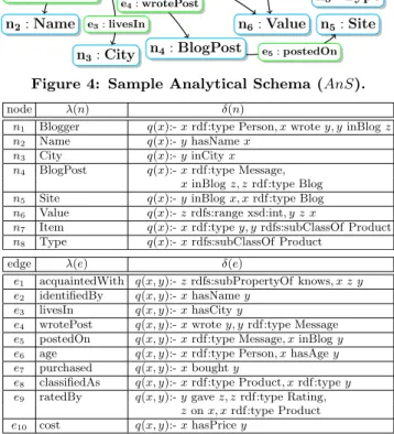
n1: Blogger e1: acquaintedWith n2: Name e2: identifiedBy n3: City e3: livesIn n4: BlogPost e4: wrotePost n5: Site e5: postedOn n6: Value e6: age n7: Item e7: purchased e9: ratedBy e10: cost n8: Type e8: classifiedAs
Figure 4: Sample Analytical Schema (AnS).
node λ(n) δ(n)
n1 Blogger q(x):- x rdf:type Person, x wrote y, y inBlog z
n2 Name q(x):- y hasName x
n3 City q(x):- y inCity x
n4 BlogPost q(x):- x rdf:type Message,
x inBlog z, z rdf:type Blog n5 Site q(x):- y inBlog x, x rdf:type Blog
n6 Value q(x):- z rdfs:range xsd:int, y z x
n7 Item q(x):- x rdf:type y, y rdfs:subClassOf Product
n8 Type q(x):- x rdfs:subClassOf Product
edge λ(e) δ(e)
e1 acquaintedWith q(x, y):- z rdfs:subPropertyOf knows, x z y
e2 identifiedBy q(x, y):- x hasName y
e3 livesIn q(x, y):- x hasCity y
e4 wrotePost q(x, y):- x wrote y, y rdf:type Message
e5 postedOn q(x, y):- x rdf:type Message, x inBlog y
e6 age q(x, y):- x rdf:type Person, x hasAge y
e7 purchased q(x, y):- x bought y
e8 classifiedAs q(x, y):- x rdf:type Product, x rdf:type y
e9 ratedBy q(x, y):- y gave z, z rdf:type Rating,
z on x, x rdf:type Product e10 cost q(x, y):- x hasPrice y
Table 1: Labels and queries of some nodes and edges of the analytical schema (AnS) shown in Figure 4. using δ we define a GAV view for each node and edge in the analytical schema. Just as an analytical schema defines (and delimits) the data available to the analyst in a typical relational DW scenario, in our framework, the classes and properties modeled by an AnS (defined using δ and labeled by λ) are the only ones visible to further RDF analytics, that is: analytical queries will be formulated against the AnS and not against the base data (as Section 4.2 will show). Exam-ple 6 introduces an AnS for the RDF graph in Figure 3.
Example 6. (Analytical Schema) Figure 4 depicts an AnS for analyzing bloggers and items. The node and edge labels appear in the figure, while the BGP queries defining these nodes and edges are provided in Table 1. In Figure 4 a blogger (n1) may have written posts (e4) which appear on some site (e5). A person may also have purchased items (e7) which can be rated (e9). The semantic of the remaining AnS nodes and edges can be easily inferred.
The nodes and edges of an analytical schema define the perspective (or lens) through which to analyze an RDF data-set. This is formalized as follows:
Definition 5. (Instance of an AnS) Let S = hN , E, λ, δi be an analytical schema and G an RDF graph. The instance of S w.r.t. G is the RDF graph I(S, G) defined as:
[ n∈N {s rdf:type λ(n) | s ∈ q(G∞) ∧ q = δ(n)} ∪ [ e∈E {s λ(e) o | s, o ∈ q(G∞) ∧ q = δ(e)}.
From now on, we denote the instance of an AnS either I(S, G) or simply I, when that does not lead to confusion.
Example 7. (Analytical Schema Instance) Below we show part of the instance of the analytical schema introduced in Example 6. We indicate at right of each triple the node (or edge) of the AnS which produced it.
I(S, G′) =
{user1rdf:type Blogger, n1
user1acquaintedWithuser2, e1
user1identifiedBy“Bill”, e2
post1postedOnblog1, e5
user1age“28”, e6
product1 rdf:type Item, n7
SmartPhone rdf:type Type, n8
product1 cost“400”, . . .} e10
Central to our notion of RDF warehouse is the disjunctive se-mantics of an AnS, materialized by the two levels of union (∪) in Definition 5. Each node and each edge of an AnS populates I through an independent RDF query, and the re-sulting triples are unioned to produce the AnS instance. Defining AnS nodes and edges independently of each other is crucial for allowing our warehouse to:
• be an actual RDF graph (in contrast to tabular data, possibly with many nulls, which would result if we attempted to fit the RDF in a relational warehouse). This addresses the requirement (i) from our motivating scenario (Section 1). It also guarantees that the AnS instance can be shared, linked, and published according to the best current Semantic Web practices;
• directly benefit from the semantic-aware SPARQL query answering provided by SPARQL engines. This answers our semantic-awareness requirement (iii), and also (iv) (ability to query the schema, notoriously ab-sent from relational DWs);
• provide as many entry points for analysis as there are AnS nodes, in line with the flexible, decentralized na-ture of RDF graph themselves (requirement (ii)). As a consequence (see below), aggregation queries are very flexible, e.g., they can aggregate one entity in relation with another (count restaurants at proximity of land-marks, requirement (v) in Section 1);
• support AnS changes easily (requirement (ii)) since nodes and/or edge definitions can be freely added to (removed from) the AnS, with no impact on the other node/edge definitions, or their instances.
As an illustration of our point on heterogeneity ((i) above), consider the three users in the original graph G (Figure 2) and their properties: user1, user2 and user3 are part of the Blogger class in our AnS instance I (through n1’s query), although user2 and user3 lack a name. However, those user properties present in the original graph, are reflected by the AnS edges e3, e4 etc. Thus, RDF heterogeneity is accepted in the base data and present in the AnS instance.
Defining analytical schemas. As customary in data anal-ysis/warehouse, analysts are in charge of defining the schema, with significant flexibility in our framework for doing so. Typically, schema definition starts with the choice of a few concepts of interest, to be turned into AnS nodes. These can come from the application, or be “suggested” based on the RDF data itself, e.g., the most popular types in the dataset (RDF classes together with the number of resources be-longing to the class), which can be obtained with a simple SPARQL query; we have implemented this in the GUI of our tool [13]. Core concepts and edges may also be identi-fied through RDF summarization as in e.g., [12]. Further, SPARQL queries can be asked to identify the most frequent
relationships to which the resources of an AnS node partic-ipate, or chains of relationships connecting instances of two AnS nodes etc. In this incremental fashion, the AnS can be “grown” from a few nodes to a graph capturing all informa-tion of interest; throughout the process, SPARQL queries can be leveraged to assist and guide AnS design.
Once the queries defining AnS nodes are known, the ana-lyst may want to check that an edge is actually connected to a node adjacent to the edge, in the sense: some resources in the node extent also participate to the relationship defined by edge. Let n1, n2∈ N be AnS nodes and en1→n2 ∈ E an
edge between them. This condition can be easily checked through a SPARQL query ensuring that:
ans(δ(n1)) ∩ Πdomain(ans(δ(en1→n2))) 6= ∅
Extensions. An AnS uses unary and binary BGP queries (introduced in Section 3) to define its instance, as the union of all AnS node/class and edge/property instances. This can be extended straightforwardly to unary and binary (full) SPARQL queries (allowing disjunction, filter, regular ex-pressions, etc.) in the setting of RDF analytics, and even to unary and binary queries from (a mix of) query languages (SQL, SPARQL, XQuery, etc.), in order to analyze data in-tegrated from distributed heterogeneous sources.
4.2
Analytical queries
Data warehouse analysis summarizes facts according to relevant criteria into so-called cubes. Formally, a cube (or analytical query) analyzes facts characterized by some di-mensions, using a measure. We consider a set of dimensions d1, d2, . . . , dn, such that each dimension di may range over the value set {d1
i, . . . , d ni
i }; the Cartesian product of all di-mensions d1× · · · × dndefines a multidimensional space M. To each tuple t in this multidimensional space M corre-sponds a subset Ft of the analyzed facts, having for each dimension di,1≤i≤n, the value of t along di.
A measure is a set of values2 characterizing each analyzed fact f . The facts in Ftare summarized by the cube cell M[t] by the result of an aggregation function ⊕ (e.g., count, sum, average, etc.) applied to the union of the measures of the Ft facts: M[t] = ⊕(Sf∈Ftvf).
An analytical query consists of two (rooted) queries and an aggregation function. The first query, known as a classifier in traditional data warehouse settings, defines the dimen-sions d1, d2, . . . , dn according to which the facts matching the query root will be analyzed. The second query defines the measure according to which these facts will be rized. Finally, the aggregation function is used for summa-rizing the analyzed facts.
To formalize the connection between an analytical query and the AnS on which it is asked, we introduce a useful notion:
Definition 6. (BGP query to AnS homomorphism) Let q be a BGP query whose labeled directed graph is Gq= hN , E, λi, and S = hN′, E′, λ′, δ′i be an AnS. An homomor-phism from q to S is a graph homomorhomomor-phism h : Gq → S, such that:
• for every n ∈ N , λ(n) = λ′(h(n)) or λ(n) is a variable; • for every en→n′ ∈ E: (i) eh(n)→h(n′)∈ E′ and
(ii) λ(en→n′) = λ′(eh(n)→h(n′)) or λ(en→n′) is a variable;
2It is a set rather than a single value, due to the structural
het-erogeneity of the AnS instance, which is an RDF graph itself: each fact may have zero, one, or more values for a given measure.
• for every e1, e2∈ E, if λ(e1) = λ(e2) is a variable, then h(e1) = h(e2);
• for n ∈ N and e ∈ E, λ(n) 6= λ(e).
The above homomorphism is defined as a correspondence from the query to the AnS graph structure, which preserves labels when they are not variables (first two items), and maps all the occurrences of a same variable labeling differ-ent query edges to the same label value (third item). Observe that a similar condition referring to occurrences of a same variable labeling different query nodes is not needed, since by definition, all occurrences of a variable in a query are mapped to the same node in the query’s graph representa-tion. The last item (independent of h) follows from the fact that the labeling function of an AnS is injective. Thus, a query with a same label for a node and an edge cannot have an homomorphism with an AnS.
We are now ready to introduce our analytical queries. In keeping with the spirit (but not the restrictions!) of clas-sical RDWs [22, 23], a classifier defines the level of data aggregation while a measure allows obtaining values to be aggregated using aggregation functions.
Definition 7. (Analytical Query) Given an analyti-cal schema S = hN , E, λ, δi, an analytianalyti-cal query (AnQ) rooted in the node r ∈ N is a triple:
Q = hc(x, d1, . . . , dn), m(x, v), ⊕i where:
• c(x, d1, . . . , dn) is a query rooted in the node rc of its graph Gc, with λ(rc) = x. This query is called the classifier of x w.r.t. the n dimensions d1, . . . , dn. • m(x, v) is a query rooted in the node rm of its graph
Gm, with λ(rm) = x. This query is called the measure of x.
• ⊕ is a function computing a value (a literal) from an input set of values. This function is called the aggre-gator for the measure of x w.r.t. its classifier. • For every homomorphism hc from the classifier to S
and every homomorphism hm from the measure to S, hc(rc) = hm(rm) = r holds.
The last item above guarantees the “well-formedness” of the analytical query, that is: the facts for which we aggre-gate the measure are indeed those classified along the desired dimensions. From a practical viewpoint, this condition can be easily and naturally guaranteed by giving explicitly in the classifier and the measure either the type of the facts to analyze, using x rdf:type λ(r), or a property describing those facts, using x λ(er→n) o with er→n∈ E. As a result, since the labels are unique in an AnS (its labeling function is injective), every homomorphism from the classifier (respec-tively the measure) to the AnS does map the query’s root node labeled with x to the AnS’s node r.
Example 8. (Analytical Query) The query below asks for the number of sites where each blogger posts, clas-sified by the blogger’s age and city:
hc(x, y1, y2), m(x, z), counti
where the classifier and measure queries are defined by: c(x, y1, y2):- x age y1, x livesIn y2
m(x, z):- x wrotePost y, y postedOn z The semantics of an analytical query is:
Definition 8. (Answer Set of an AnQ) Let I be the instance of an AnS with respect to some RDF graph. Let Q = hc(x, d1, . . . , dn), m(x, v), ⊕i be an AnQ against I. The answer set of Q against I, denoted ans(Q, I), is:
ans(Q, I) = {hdj 1, . . . , d j n, ⊕(q j(I))i | hxj, dj 1, . . . , d j ni ∈ c(I) and qj is defined as qj(v):- m(xj, v)} assuming that each value returned by qj(I) is of (or can be converted by the SPARQL rules [35] to) the input type of the aggregator ⊕. Otherwise, the answer set is undefined.
In other words, the analytical query returns each tuple of dimension values found in the answer of the classifier query, together with the aggregated result of the measure query. The answer set of an AnQ can thus be represented as a cube of n dimensions, holding in each cube cell the corresponding aggregate measure. In the following, we focus on analytical queries whose answer sets are not undefined.
Example 9. (Analytical Query Answer) Consider the query in Example 8, over the AnS in Figure 4. Some triples from the instance of this analytical schema were shown in Example 7. The classifier query’ answer set is:
{huser1, 28, “M adrid”i, huser3, 35, “N Y ”i} while that of the measure query is:
{huser1, blog1i, huser1, blog2i, huser2, blog2i, huser3, blog2i} Aggregating the blogs among the classification dimensions leads to the AnQ answer:
{h28, “M adrid”, 2i, h35, “N Y ”, 1i}
In this work, for the sake of simplicity, we assume that an analytical query has only one measure. However, this can be easily relaxed, by introducing a set of measure queries with an associated set of aggregation functions.
5.
ANALYTICAL QUERY ANSWERING
We now consider practical strategies for AnQ answering. The AnS materialization approach. The simplest meth-od consists of materializing the instance of the AnS (Defini-tion 5) and storing it within an RDF data management sys-tem (or RDF-DM, for short); recall that the AnS instance is an RDF graph itself defined using GAV views. Then, to answer an AnQ, one can use the RDF-DM to process the classifier and measure queries, and the final aggregation. While effective, this solution has the drawback of storing the whole AnS instance; moreover, this instance may need maintenance when the analyzed RDF graph changes. The AnQ reformulation approach. To avoid materi-alizing and maintaining the AnS instance, we consider an alternative solution. The idea is to rewrite the AnQ using the GAV views of the AnS definition, so that evaluating the reformulated query returns exactly the same answer as if materialization was used. Using query rewriting, one can store the original RDF graph into an RDF-DM, and use this RDF-DM to answer the reformulated query.
Our reformulation technique below translates standard query rewriting usingGAVviews [19] to our RDF analytical setting.
Definition 9. (AnS-reformulation of a query) Given an analytical schema S = hN , E, λ, δi, a BGP query q(¯x):- t1, . . . , tm whose graph is Gq = hN′, E′, λ′i, and the non-empty set H of all the homomorphisms from q to S, the reformulation of q w.r.t. S is the union of join queries q✶
S =Sh∈Hqh✶(¯x) :-Vm
i=1qi(¯xi) such that:
• for each triple ti∈ q of the form s rdf:type λ′(ni), qi(¯xi) in qh✶is defined as qi= δ(h(ni)) and ¯xi= s; • for each triple ti∈ q of the form s λ′(ei) o,
This definition states that for a BGP query stated against an AnS, the reformulated query amounts to translating all its possible interpretations w.r.t. the AnS (modeled by all the homomorphisms from the query to the AnS) into a union of join queries modeling them. The important point is that these join queries are defined onto the RDF graph over which the AnS is wrapped.
Example 10. (AnS-reformulation of a query) Let q(x, y1) be a BGP query referring to the AnS in Figure 4.
q(x, y1):- x rdf:type Blogger, x acquaintedWith y1 The first atom x rdf:type Blogger in q is of the form srdf:type λ(n1), for the node n1.Consequently, q✶S contains as a conjunct the query:
q(x):- x rdf:type Person, x wrote y, y inBlog z obtained from δ(n1) in Table 1.
The second atom in q, x acquaintedWith y is of the form sλ(e1) o for the edge e1in Figure 4, while the query defining e1 is: q(x, y):- z rdfs:subPropertyOf knows, x z y. As a result, q✶
S contains the conjunct:
q(x, y1):- z1 rdfs:subPropertyOf knows, x z1 y1 Thus, the reformulated query amounts to:
q✶
S(x, y1):- x rdf:type Person, x wrote y, y inBlog z, z1 rdfs:subPropertyOf knows, x z1 y1 which can be evaluated directly on the graph G in Figure 2.
Theorem 1 states how BGP query reformulation w.r.t. an AnS can be used to answer analytical queries correctly.
Theorem 1. (Reformulation-based answering) Let S be an analytical schema, whose instance I is defined w.r.t. an RDF graph G. Let Q = hc(x, d1, . . . , dn), m(x, v), ⊕i be an analytical query against S, c✶
S be the reformulation of Q’s classifier query against S, and m✶
S be the reformulation of Q’s measure query against S. We have:
ans(Q, I) = {hdj1, . . . , djn, ⊕(qj(G∞))i | hxj, dj1, . . . , djni ∈ c✶S(G∞)
and qj is defined as qj(v):- m✶ S(xj, v)}
assuming that each value returned by qj(G∞) is of (or can be converted by the SPARQL rules [35] to) the input type of the aggregator ⊕. Otherwise, the answer set is undefined.
The theorem states that in order to answer Q on I, one first reformulates Q’s classifier into c✶
Sand answers it directly against G (not against I as in Definition 8): this is how reformulation avoids materializing I. Then, for each tuple hxj, dj
1, . . . , djni returned by the classifier, the following steps are applied: instantiate the reformulated measure query m✶ S with the fact xj, leading to the query qj; answer the latter against G; finally, aggregate its results through ⊕. The proof follows directly, by two-way inclusion.
The trade-offs between materialization and reformulation have been thoroughly analyzed in the literature [22]; we leave the choice to the RDF warehouse administrator.
6.
OLAP RDF ANALYTICS
On-Line Analytical Processing (OLAP) [3] technologies enhance the abilities of data warehouses (so far, mostly re-lational) to answer multi-dimensional analytical queries.
The analytical model we introduced is specifically designed for graph-structured, heterogeneous RDF data. In this sec-tion, we demonstrate that our model is able to express RDF-specific counterparts of all the traditional OLAP concepts and tools known from the relational DW setting.
Typical OLAP operations allow transforming a cube into another. In our framework, a cube corresponds to an AnQ; for instance, the query in Example 8 models a bi-dimensional cube on the warehouse related to our sample AnS in Figure 4. Thus, we model traditional OLAP operations on cubes as AnQ rewritings, or more specifically, rewritings of extended AnQs which we introduce below:
Definition 10. (Extended AnQ) As in Definition 7, let S be an AnS, and d1, . . . , dn be a set of dimensions, each ranging over a non-empty finite set Vi,1≤i≤n. Let Σ be a total function over {d1, . . . , dn} associating to each di, either {di} or a non-empty subset of Vi. An extended analytical query Q is defined by a triple:
Q:- hcΣ(x, d1, . . . , dn), m(x, v), ⊕i
where (as in Definition 7) c is a classifier and m a measure query over S, ⊕ is an aggregation operator, and moreover:
cΣ(x, d1, . . . , dn) = S
(χ1,...,χn)∈Σ(d1) × ...×Σ(dn)c(x, χ1, . . . , χn)
In the above, the extended classifier cΣ(x, d1, . . . , dn) is the set of all possible classifiers obtained by substituting each dimension variable diwith a value in Σ(di). The function Σ is introduced to constrain some classifier dimensions, i.e., it plays the role of a filter-clause restricting the classifier re-sult. The semantics of an extended analytical query is easily derived from the semantics of a standard AnQ (Definition 8) by replacing the tuples from c(I) with tuples from cΣ(I). In other words, an extended analytical query can be seen as a union of a set of standard AnQs, one for each combination of values in Σ(d1), . . . , Σ(dn). Conversely, an analytical query corresponds to an extended analytical query where Σ only contains pairs of the form (di, {di}).
We can now define the classical slice and dice OLAP op-erations in our framework:
Slice. Given an extended query Q = hcΣ(x, d1, . . . , dn), m(x, v), ⊕i, a slice operation over a dimension diwith value vireturns the extended query hcΣ′(x, d1, . . . , dn), m(x, v), ⊕i, where Σ′= (Σ \ { (di, Σ(di)) }) ∪ { (di, {vi}) }.
The intuition is that slicing binds an aggregation dimen-sion to a single value.
Example 11. (Slice) Let Q be the extended query cor-responding to the query-cube defined in Example 8, that is: hcΣ(x, y1, y2), m(x, z), counti, Σ = { (y1, {y1}), (y2, {y2}) } (the classifier and measure are as in Example 8). A slice operation on the age dimension y1 with value 35 results in replacing the extended classifier of Q with cΣ′(x, y1, y2) = {c(x, 35, y2)} where Σ′= Σ \ { (y1, {y1}) } ∪ { (y1, {35}) }. Dice. Similarly, a dice operation on Q over dimensions {di1, . . . , dik} and corresponding sets of values {Si1, . . . , Sik},
returns the query hcΣ′(x, d1, . . . , dn), m(x, v), ⊕i, where Σ′= (Σ \Sik
j=i1{ (dj, Σ(dj)) }) ∪
Sik
j=i1{ (dj, Sj) }.
Intuitively, dicing forces several aggregation dimensions to take values from specific sets.
Example 12. (Dice) Consider again the initial cube Q from Example 8 and a dice operation on both age and location dimensions with values {28} for y1 and {Madrid, Kyoto} for y2. The dice operation replaces the extended classifier of Q with cΣ′(x, y1, y2) = {c(x, 28, “Madrid”), c(x, 28, “Kyoto”)} where Σ′ = Σ \ { (y
1, {y1}), (y2, {y2}) } ∪ { (y1, {28}), (y2, {“Madrid”, “Kyoto”}) }.
Drill-in and drill-out. These operations consist of adding and removing a dimension to the classifier, respectively. Rewritings for drill operations can be easily formalized. Due to space limitations we omit the details, and instead exem-plify below a drill-in example.
Example 13. (Drill-in) Consider the cube Q from Ex-ample 8, and a drill-in on the age dimension. The drill-in rewriting produces the query Q = hc′Σ′(x, y2), m(x, z), counti with Σ′= { (y2, {y2}) } and c′(x, y2) = x livesIn y2. Dimension hierarchies. Typical relational warehousing scenarios feature hierarchical dimensions, e.g., a value of the country dimension corresponds to several regions, each of which contains many cities etc. Such hierarchies were not considered in our framework thus far3.
To capture hierarchical dimensions, we introduce dedi-cated built-in properties to model the nextLevel relation-ship among parent-child dimensions in a hierarchy. For il-lustration, consider the addition of a new State node and a new nextLevel edge to the AnS in Figure 4. Below, only part of that AnS is shown, highlighting the new nodes and edges with dashed lines:
n1: Blogger n2: Name e2: identifiedBy n3: City e3: livesIn n9: State e11: nextLevel n4: BlogPost e4: wrotePost n 5: Site e5: postedOn n6: Value e6: age
In a similar fashion one could use the nextLevel prop-erty to support hierarchies among edges. For instance, relationships such as isFriendsWith and isCoworkerOf can be rolled up into a more general relationship knows etc.
Based on dimension hierarchies, roll-up/drill-down oper-ations correspond to adding to/removing from the classifier, triple atoms navigating such nextLevel edges.
Example 14. (Roll-up) Recall the query in Example 8. A roll-up along the City dimension to the State level yields hc′
Σ′(x, y1, y3), m(x, z), counti, where:
c′Σ′(x, y1, y3):- x age y1, x livesIn y2, y2 nextLevel y3. The measure component remains the same, and Σ′ in the rolled-up query consists of the obvious pairs of the form (d, {d}). Note the change in both the head and body of the classifier, due to the roll-up.
7.
EXPERIMENTS
We demonstrate the performance of our RDF analytical framework through a set of experiments. Section 7.1 outlines our implementation and experimental settings. We describe experiments on I materialization in Section 7.2, evaluate AnQs in Section 7.3 and OLAP operations in Section 7.4, then we conclude. Due to space limitation, experiments per-formed with query reformulation are delegated to [14].
7.1
Implementation and settings
We implemented the concepts and algorithms presented above within our WaRG tool [13]. WaRG is built on top of
kdb+v3.0 (64 bits) [2], an in-memory column DBMS used in decision-support analytics. kdb+provides arrays (tables), which can be manipulated through theq interpreted pro-gramming language. We store in kdb+ the RDF graph G, 3Dimension hierarchies should not be confused with the
hier-archies built using the predefined RDF(S) properties, such as rdfs:subClassOf, e.g., in Figure 2.
Tables used forAnS materialization
Tables used forAnQ reformulation
dict (URI encodings) uri[str], val[int] AnS instance dw (DW instance: I)
s[int], p[int], o[int] OR nX (I nodes) s[int] eY (I edges) s[int], o[int] AnS definition asch (DW schema: AnS)
s[int], p[int], o[int]
query dict (AnS nodes/edges) λ[int], δ[str] RDF graph db (RDF/S triples)
s[int], p[int], o[int]
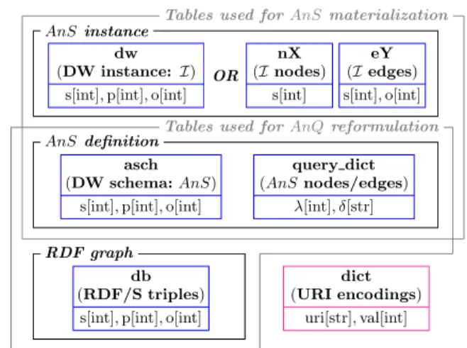
Figure 5: Data layout of the RDF warehouse.
Gsize schema size dictionary G∞size 3.4 × 10⁷triples, 5.5 × 10³triples, 7 × 10⁶ 3.8 × 10⁷
4.4 GB 746 KB entries triples
Table 2: Dataset characteristics.
the AnS definitions, as well as the AnS instance, when we choose to materialize it. We translate BGP queries into q
programs thatkdb+ interprets; any engine capable of stor-ing RDF and processstor-ing conjunctive RDF queries could be easily used instead.
Data organization. Figure 5 illustrates our data layout in kdb+. The URIs within the RDF dataset are encoded using integers; the mapping is preserved in a q dictionary data structure, named dict. The saturation of G, denoted G∞(Section 3), is stored in the db table. Analytical schema definitions are stored as follows. The asch table stores the analytical schema triples: λ(n) λ(en→n′) λ(n′). The
sepa-rate query dict dictionary maps the labels λ for nodes and edges to their corresponding queries δ. Finally, we use the dw table to store the AnS instance I, or several tables of the form nX and eY if a partitioned-table storage is used (see Section 7.2). While query dict and db suffice to cre-ate the instance, we store the analytical schema definition in asch to enable checking incoming analytical queries for correctness w.r.t. the AnS.
kdb+ stores each table column independently, and does not have a database-style query optimizer. It is quite fast since it is an in-memory system; at the same time, it relies on theqprogrammer’s skills for obtaining an efficient execu-tion. We try to avoid low-performance formulations of our queries inq, but further optimization is possible and more elaborate techniques (e.g., cost-based join reordering etc.) would further improve performance.
Dataset. Our experiments used the Ontology and Ontology Infobox datasets from the DBpedia Download 3.8; the data characteristics are summarized in Table 2. For our scalability experiments (Section 7.2), we replicated these datasets to study scalability in the database size.
Hardware. The experiments ran on an 8-core DELL server at 2.13 GHz with 16 GB of RAM, running Linux 2.6.31.14. All times we report are averaged over five executions.
7.2
Analytical schema materialization
Loading the (unsaturated) G took about 3 minutes, and computing its full saturation G∞ 22 minutes. We designed an AnS of 26 nodes and 75 edges, capturing a set of concepts
A rt is tS ci e n ti s t (2 ) A g e n t (1 ) A rt is t (1 ) A w a rd ( 1 ) Co m p a n y ( 1 ) C u rr e n cy ( 1 ) E th n ic G ro u p ( 1 ) E d u In s ti tu tio n ( 1 ) G o v T y p e ( 1 ) Id e o lo g y (1 ) L a n g u a g e ( 1 ) N o n -P ro fi tO rg ( 1 ) O rg a n is a ti o n ( 1 ) P e rs o n ( 1 ) P e rs o n F u n ct io n ( 1 ) P o p u la te d P la ce ( 1 ) P ro g L a n g u a g e ( 1 ) S c ie n ti s t (1 ) S o ft w a re ( 1 ) W o rk ( 1 ) W ri tt e n W o rk ( 1 ) D o u b le ( 2 ) Y e a r (2 ) S tr in g ( 2 ) 0 0.2 0.4 0.6
lo g10 (nu mber of resu lts) / 10 eva lua tion u sing d w (s) eva lua tion u sing p artitio ned store (s )
a ff ili a tio n ( 3 ) b ir th P la ce O f (1 ) c o n tr ib u te W o rk ( 3 ) h e a d O f (3 ) p e rs o n F u n ct io n ( 3 ) p la ce L a n g u a g e ( 3 ) re la te d C o m p a n y (3 ) re la te d P e rso n ( 3 ) re la te d W o rk (3 ) w o rkL a n g u a g e ( 3 ) w o rk R lt d P e rso n ( 3 ) a re a T o ta l (1 ) b ir th P la c e ( 1 ) d e a th P la ce ( 1 ) o c c u p a tio n ( 1 ) p o p u la ti o n T o ta l (1 ) st a rr in g ( 1 ) w ri te r (1 ) 0.01 0.1 1 10
Figure 6: Evaluation time (s) and number of results for AnS node queries (left) and edge queries (right).
38 x 10^60 71 x 10^6 104 x 10^6 137 x 10^6 169 x 10^6 50 100 150 200 250 300
dictionary size (number of triples / 10^6) instance size (number of triples / 10^6) time to create instance table (s) time to create partitioned tables (s)
initial graph size (number of triples)
Figure 7: I materialization time vs. I size. and relationship of interest. AnS node queries have one or two atoms, while edge queries consist of one to three atoms. We considered two ways of materializing the instance I. First, we used a single table (dw in Figure 5). Second, in-spired from RDF stores such as [21], we tested a partitioned data layout for I as follows. For each distinct node (model-ing triples of the form s rdf:type λX), we store a table with the subjects s declared of that type; this leads to a set of ta-bles denoted nX (for node), with X ∈ [1, 26]. Similarly, for each distinct edge (s λY o) a separate table stores the cor-responding triple subjects and objects, leading to the tables eY with Y ∈ [1, 75].
Figure 6 shows for each node and edge query (labeled on the y axis by λ, chosen based on the name of a “central” class or property in the query): (i) the number of query atoms (in parenthesis next to the label), (ii) the number of query re-sults (we show log10(#res)/10 to improve readability), (iii) the evaluation time when inserting into a single dw table, and (iv) the time when inserting into the partitioned store. For 2 node queries and 57 edge queries, the evaluation time is too small to be visible (below 0.01 s), and we omitted them from the plots. The total time to materialize the instance I (1.3 × 10⁷ triples) was 38 seconds.
Scalability. We created larger RDF graphs such that the size of I would be multiplied by a factor of 2 to 5, with respect to the I obtained from the original graph G. The corresponding I materialization time are shown in Figure 7, demonstrating linear scale-up w.r.t. the data size.
7.3
Analytical query answering over
IWe consider a set of AnQs, each adhering to a specific query pattern. A pattern is a combination of: (i) the number of atoms in the classifier query (denoted c), (ii) the number of dimension variables in the classifier query (denoted v), and (iii) the number of atoms in the measure query (de-noted m). For instance, the pattern c5v4m3 designates queries whose classifiers have 5 atoms, aggregate over 4 di-mensions, and whose measure queries have 3 atoms. We used 12 distinct patterns for a total of 1,097 queries.
c1 v1 m 1 c1 v1 m 2 c1 v1 m 3 c2 v1 m 3 c3 v2 m 3 c4 v3 m 3 c5 v1 m 3 c5 v2 m 3 c5 v3 m 3 c5 v4 m 1 c5 v4 m 2 c5 v4 m 3 0 1 10
average minimum maximum
c1v1m1 (73) c1v1m2 (53) c1v1m3 (62) c2v1m3 (71) c3v2m3 (76) c4v3m3 (130) c5v1m3 (144) c5v2m3 (216) c5v3m3 (144) c5v4m1 (28) c5v4m2 (64) c5v4m3 (36) 0 1 10 100 1,000 10,000 100,000 e va lu a ti o n t im e ( s) n u m b e r o f re su lt s
Figure 8: AnQ statistics for query patterns.
0 2 4 6 8 0 2 4 6 8 instance table partitioned store e va lu a ti o n t im e ( s) c1v1m1 c5v4m3
instance size (number of triples)
Figure 9: AnQ evaluation time over large datasets. The graph at the top of Figure 8 shows for each query pat-tern, the number of queries in the set (in parenthesis after the pattern name), and the average, minimum and maxi-mum number of query results. The largest result set (for c4v3m3) is 514, 240, while the second highest (for c1v1m3) is 160, 240. The graph at the bottom of Figure 8 presents the average, minimum and maximum query evaluation times among the queries of each pattern.
Figure 8 shows that query result size (up to hundreds of thousands) is the most strongly correlated with query eval-uation time. Other parameters impacting the evaleval-uation time are the number of atoms in the classifier and measure queries, and the number of aggregation variables. These parameters are to be expected in an in-memory execution engine such as kdb+. Observe the moderate time increase with the main query size metric (the number of atoms); this demonstrates robust performance even for complex AnQs.
Figure 9 shows the average evaluation time for queries belonging to the sets c1v1m1 and c5v4m3 over increasing tables, using the instance triple table and the partitioned store implementations. In both cases the evaluation time increases linearly with the size of the dataset. The graph shows that the partitioned store brings a modest speed-up (about 10%); for small queries, the difference is
unnotice-Q 1 Q 1 s 1 Q 1 s 2 Q 1 s 3 Q 1 s 4 Q 1 d 1 Q 1 d 2 Q 1 d 3 Q 1 d 4 Q 2 Q 2 s 1 Q 2 s 2 Q 2 s 3 Q 2 s 4 Q 2 d 1 Q 2 d 2 Q 2 d 3 Q 2 d 4 Q 3 Q 3 s 1 Q 3 s 2 Q 3 s 3 Q 3 s 4 Q 3 d 1 Q 3 d 2 Q 3 d 3 Q 3 d 4 0 1 2 3 4 5 6 7
log10 (number of answers) evaluation time (s)
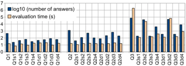
Figure 10: Slice and dice over AnQs.
able. Thus, without loss of generality, in the sequel we con-sider only the single-table dw option.
7.4
OLAP operations
We now study the performance of OLAP operations on analytical queries (Section 6).
Slice and dice. In Figure 10, we consider three c5v4m3 queries: Q1 having a small result size (455), Q2 with a medium result size (1, 251) and Q3 with a large result size (73, 242). For each query we perform a slice (dice) by re-stricting the number of answers for each of its 4 dimension variables, leading to the OLAP queries Q1s1to Q1s4, Q1d1to Q1d4and similarly for Q2and Q3. The figure shows that the slice/dice running time is strongly correlated with the result size, and is overall small (under 2 seconds in many cases, 4 seconds for Q3 slice and dice queries having 104results). Drill-in and drill-out. The queries following the patterns c5v1m3, c5v2m3, c5v3m3 and c5v4m3 were chosen start-ing from the ones for c5v4m3 and eliminatstart-ing one dimen-sion variable from the classifier (without any other change) to obtain c5v3m3; removing one further dimension variable yielded the c5v2m3 queries etc. Recalling the definitions of drill-in and drill-out (Section 6), it follows that the queries in c5vnm3 are drill-ins of c5v(n+1)m3 for 1≤n≤3, and conversely, c5v(n+1)m3 result from drill-out on c5vnm3. Their evaluation times appear in Figure 8.
7.5
Conclusion of the experiments
Our experiments demonstrate the feasibility of our full RDF warehousing approach, which exploits standard RDF functionalities such as triple storage, conjunctive query eval-uation, and reasoning. We showed robust scalable perfor-mance when loading and saturating G, and building I in time linear in the input size (even for complex, many-joins node and edge queries). Finally, we proved that OLAP operations can be evaluated quite efficiently in our RDF cube (AnQ) context. While further optimizations are possible, our ex-periments confirmed the interest and good performance of our proposed all-RDF Semantic Web warehousing approach. Perspective: OLAP operations evaluated on AnQs. The OLAP operations described thus far were applied on AnQs and evaluated against I. We are interested in im-proving performance of such operations by evaluating them directly on the materialized results of previous analytical queries (significantly reducing the input data and benefiting from the regular-structure AnQ results). We plan to analyze the situations where such “shortcuts” are applicable.
8.
RELATED WORK
Relational warehousing has been well studied [23, 22]. Web data warehouses have been presented as interconnected corpora of XML documents and Web services [5], or as dis-tributed knowledge bases [6]. In [30], a large RDF knowledge
base, Yago [32], is enriched with information gathered from the Web. These works did not consider RDF analytics.
[16, 34] propose RDF(S) vocabularies (pre-defined classes and properties) for describing relational multidimensional data in RDF; [16] also maps OLAP operations into SPARQL queries. [27] presents a semi-automated approach for deriv-ing a RDW from an ontology. In contrast with the above, in our approach, the AnS instance is an RDF graph itself thus seamlessly preserves the heterogeneity, semantics, and ability to query the schema with the data present in RDF.
In the area of RDF data management, previous works focused on efficient stores [4, 11, 31], indexing [36], query processing [28] and multi-query optimization [26], view se-lection [17] and query-view composition [25], or Map-Reduce based RDF processing [20, 21]. BGP query answering tech-niques have been studied intensively, e.g., [18, 29], and some are deployed in commercial systems such as Oracle 11g, which provides a “Semantic Graph” extension etc. Our work defines a novel framework for RDF analytics, based on analytical schemas and queries; these can be efficiently de-ployed on top of any RDF data management platform, to extend it with analytic capabilities.
Analysis cubes and OLAP operations on cubes over graphs are also defined in [40]. However, their approach does not handle heterogeneous graphs, and thus it cannot handle multi-valued attributes (e.g., a movie being both a comedy and a romance), nor data semantics, both central in RDF. Further, their approach only focuses on counting edges in contrast with our flexible AnQ (Section 4.2).
In [10], graph data can be aggregated in a spatial fashion by grouping connected nodes into regions (think of a street map graph); based on this simple aggregation, an OLAP framework is built. Beyond being RDF-specific (unlike [10]), our framework also introduces analytical graph schemas, and allows for much more general aggregation.
[24] proposes techniques for transforming OLAP queries into SPARQL. Query answering is optimized by materializ-ing data cubes. Such processmaterializ-ing can be added to our frame-work in order to further optimize AnQ answering.
The separation between grouping and aggregation present in our AnQs is similar to the MD-join operator [9] for RDWs. Finally, SPARQL 1.1 [35] features SQL-style grouping and aggregation. Deploying our framework on an efficient SPARQL 1.1 platform enables taking advantage both of its efficiency and of the high-level, expressive, flexible RDF graph analysis concepts introduced in this work.
9.
CONCLUSION
DW models and techniques have had a strong impact on the usages and usability of data. In this work, we proposed the first approach for specifying and exploiting an RDF data warehouse, notably by (i) defining an analytical schema that captures the information of interest, and (ii) formalizing an-alytical queries (or cubes) over the AnS. Importantly, in-stances of AnS are RDF graphs themselves, which allows to exploit the semantics and rich, heterogeneous structure (e.g., jointly query the schema and the data) that make RDF data rich and interesting.
The broader area of data analytics, related to data ware-housing, albeit with a significantly extended set of goals and methods, is the target of very active research now, especially in the context of massively parallel Map-Reduce processing etc. Efficient methods for deploying AnSs and AnQ evalu-ation in such a parallel context are part of our future work.
10.
REFERENCES
[1] The DBpedia Knowledge Base. http://dbpedia.org. [2] [kx] white paper.
kx.com/papers/KdbPLUS Whitepaper-2012-1205.pdf. [3] OLAP council white paper.
http://www.olapcouncil.org/research/resrchly.htm. [4] D. J. Abadi, A. Marcus, S. R. Madden, and
K. Hollenbach. Scalable semantic web data management using vertical partitioning. In VLDB, 2007.
[5] S. Abiteboul. Managing an XML warehouse in a P2P context. In CAiSE, 2003.
[6] S. Abiteboul, E. Antoine, and J. Stoyanovich. Viewing the web as a distributed knowledge base. In ICDE, 2012.
[7] S. Abiteboul, R. Hull, and V. Vianu. Foundations of Databases. Addison-Wesley, 1995.
[8] S. Abiteboul, I. Manolescu, P. Rigaux, M.-C. Rousset, and P. Senellart. Web Data Management and
Distribution. Cambridge University Press, Dec 2011. [9] M. Akinde, D. Chatziantoniou, T. Johnson, and
S. Kim. The MD-join: An operator for complex OLAP. In ICDE, pages 524–533, 2001.
[10] D. Bleco and Y. Kotidis. Business intelligence on complex graph data. In EDBT/ICDT Workshops, 2012.
[11] M. A. Bornea, J. Dolby, A. Kementsietsidis, K. Srinivas, P. Dantressangle, O. Udrea, and
B. Bhattacharjee. Building an efficient RDF store over a relational database. In SIGMOD Conference, pages 121–132, 2013.
[12] S. Campinas, T. E. Perry, D. Ceccarelli, R. Delbru, and G. Tummarello. Introducing RDF graph summary with application to assisted SPARQL formulation. 2012 23rd International Workshop on Database and Expert Systems Applications, 0:261–266, 2012.
[13] D. Colazzo, T. Ghosh, F. Goasdou´e, I. Manolescu, and A. Roati¸s. WaRG: Warehousing RDF Graphs
(demonstration). In Bases de Donn´ees Avanc´ees (informal national French conference, no proceedings), 2013. See https://team.inria.fr/oak/warg/. [14] D. Colazzo, F. Goasdou´e, I. Manolescu, and A. Roati¸s.
Warehousing RDF graphs. In Bases de Donn´ees Avanc´ees (informal national French conference, no proceedings), 2013.
[15] O. Erling and I. Mikhailov. RDF Support in the Virtuoso DBMS. Networked Knowledge - Networked Media, pages 7–24, 2009.
[16] L. Etcheverry and A. A. Vaisman. Enhancing OLAP analysis with web cubes. In ESWC, 2012.
[17] F. Goasdou´e, K. Karanasos, J. Leblay, and I. Manolescu. View selection in Semantic Web databases. PVLDB, 5(1), 2012.
[18] F. Goasdou´e, I. Manolescu, and A. Roati¸s. Efficient query answering against dynamic RDF databases. In International Conference on Extending Database Technology, pages 299–310, 2013.
[19] A. Y. Halevy. Answering queries using views: A survey. VLDB J., 10(4):270–294, 2001.
[20] J. Huang, D. J. Abadi, and K. Ren. Scalable SPARQL Querying of Large RDF Graphs. PVLDB, 4(11), 2011.
[21] M. Husain, J. McGlothlin, M. M. Masud, L. Khan, and B. M. Thuraisingham. Heuristics-Based Query Processing for Large RDF Graphs Using Cloud Computing. IEEE Trans. on Knowl. and Data Eng., 2011.
[22] M. Jarke, M. Lenzerini, Y. Vassiliou, and
P. Vassiliadis. Fundamentals of Data Warehouses. Springer, 2001.
[23] C. S. Jensen, T. B. Pedersen, and C. Thomsen. Multidimensional Databases and Data Warehousing. Synthesis Lectures on Data Management. Morgan & Claypool Publishers, 2010.
[24] B. K¨ampgen and A. Harth. No size fits all – running the star schema benchmark with SPARQL and RDF aggregate views. In ESWC 2013, LNCS 7882, pages 290–304, Heidelberg, Mai 2013. Springer.
[25] W. Le, S. Duan, A. Kementsietsidis, F. Li, and M. Wang. Rewriting queries on SPARQL views. In WWW, pages 655–664, 2011.
[26] W. Le, A. Kementsietsidis, S. Duan, and F. Li. Scalable multi-query optimization for SPARQL. In ICDE, pages 666–677, 2012.
[27] V. Nebot and R. B. Llavori. Building data warehouses with semantic web data. Decision Support Systems, 52(4), 2012.
[28] T. Neumann and G. Weikum. The RDF-3X engine for scalable management of RDF data. VLDB J., 19(1), 2010.
[29] J. P´erez, M. Arenas, and C. Gutierrez. nSPARQL: A navigational language for RDF. J. Web Sem., 8(4):255–270, 2010.
[30] N. Preda, G. Kasneci, F. M. Suchanek, T. Neumann, W. Yuan, and G. Weikum. Active knowledge: dynamically enriching RDF knowledge bases by web services. In SIGMOD, 2010.
[31] L. Sidirourgos, R. Goncalves, M. Kersten, N. Nes, and S. Manegold. Column-store support for RDF data management: not all swans are white. PVLDB, 1(2), 2008.
[32] F. M. Suchanek, G. Kasneci, and G. Weikum. YAGO: A large ontology from Wikipedia and WordNet. J. Web Sem., 6(3), 2008.
[33] W3C. Resource description framework. http://www.w3.org/RDF/.
[34] W3C. The RDF data cube vocabulary.
http://www.w3.org/TR/vocab-data-cube/, 2012. [35] W3C. SPARQL 1.1 query language.
http://www.w3.org/TR/sparql11-query/, March 2013. [36] C. Weiss, P. Karras, and A. Bernstein. Hexastore:
sextuple indexing for Semantic Web data management. PVLDB, 1(1), 2008. [37] Jena. http://jena.sourceforge.net. [38] Owlim. http://owlim.ontotext.com. [39] Sesame. http://www.openrdf.org.
[40] P. Zhao, X. Li, D. Xin, and J. Han. Graph cube: on warehousing and OLAP multidimensional networks. In SIGMOD, pages 853–864, 2011.