Dual-Paradigm Stream Processing

HAL Id: hal-01834668

https://hal.inria.fr/hal-01834668

Submitted on 21 Sep 2018

HAL is a multi-disciplinary open access

archive for the deposit and dissemination of

sci-entific research documents, whether they are

pub-lished or not. The documents may come from

teaching and research institutions in France or

abroad, or from public or private research centers.

L’archive ouverte pluridisciplinaire HAL, est

destinée au dépôt et à la diffusion de documents

scientifiques de niveau recherche, publiés ou non,

émanant des établissements d’enseignement et de

recherche français ou étrangers, des laboratoires

publics ou privés.

Dual-Paradigm Stream Processing

Song Wu, Zhiyi Liu, Shadi Ibrahim, Lin Gu, Hai Jin, Fei Chen

To cite this version:

Song Wu, Zhiyi Liu, Shadi Ibrahim, Lin Gu, Hai Jin, et al.. Dual-Paradigm Stream Processing.

ICPP 2018 - 47th International Conference on Parallel Processing, Aug 2018, Eugene, United States.

pp.Article No. 83, �10.1145/3225058.3225120�. �hal-01834668�

Song Wu

SCTS/CGCL

Huazhong University of Science and Technology

Wuhan, China wusong@hust.edu.cn

Zhiyi Liu

SCTS/CGCL

Huazhong University of Science and Technology

Wuhan, China zhiyiliu@hust.edu.cn

Shadi Ibrahim

Inria, IMT Atlantique, LS2N Nantes, France shadi.ibrahim@inria.fr

Lin Gu

SCTS/CGCL

Huazhong University of Science and Technology

Wuhan, China lingu@hust.edu.cn

Hai Jin

SCTS/CGCL

Huazhong University of Science and Technology

Wuhan, China hjin@hust.edu.cn

Fei Chen

SCTS/CGCL

Huazhong University of Science and Technology

Wuhan, China fei_chen_2013@hust.edu.cn

ABSTRACT

Existing stream processing frameworks operate either under data stream paradigm processing data record by record to favor low latency, or under operation stream paradigm processing data in micro-batches to desire high throughput. For complex and mutable data processing requirements, this dilemma brings the selection and deployment of stream processing frameworks into an embarrass-ing situation. Moreover, current data stream or operation stream paradigms cannot handle data burst efficiently, which probably re-sults in noticeable performance degradation. This paper introduces a dual-paradigm stream processing, called DO (Data and Operation) that can adapt to stream data volatility. It enables data to be pro-cessed in micro-batches (i.e., operation stream) when data burst occurs to achieve high throughput, while data is processed record by record (i.e., data stream) in the remaining time to sustain low latency. DO embraces a method to detect data bursts, identify the main operations affected by the data burst and switch paradigms accordingly. Our insight behind DO’s design is that the trade-off between latency and throughput of stream processing frameworks can be dynamically achieved according to data communication among operations in a fine-grained manner (i.e., operation level) instead of framework level. We implement a prototype stream pro-cessing framework that adopts DO. Our experimental results show that our framework with DO can achieve 5x speedup over operation stream under low data stream sizes, and outperforms data stream on throughput by 2.1x to 3.2x under data burst.

KEYWORDS

Stream processing, Dual-paradigm approach, Data burst, Low la-tency, High throughput

1

INTRODUCTION

Stream data processing is widely adopted in many domains includ-ing stock market, fraud detection, electronic tradinclud-ing, Internet of Things (IOT), etc. [20]. This broad adoption results in the prolifera-tive demand of stream data processing frameworks such as Spark

∗_{The corresponding author}

Streaming [28], Flink [12], Storm [22]. Different stream data process-ing frameworks provide different advantages, e.g., high throughput or low latency.

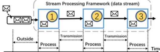
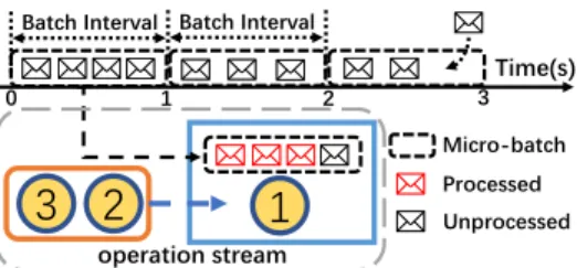
In particular, there are two main types of paradigms in stream processing, i.e., data stream and operation stream. Data stream is widely adopted by most existing stream processing frameworks, e.g., S4 [17], MillWheel [1], Naiad [16], Samza [19], Storm [22], Flink [12], and Heron [14]. Data stream fixes operations in certain workers and schedules data to flow through these operations, as illustrated in Figure 1(a). Note that data stream processes data in a single-record-at-a-time manner, towards low latency but also with low throughput. In contrast, operation stream fixes the data into the workers and schedules the operations, as illustrated in Figure 1(b). It accumulates a certain number of records during a time interval to form a micro-batch and then process it, i.e., batch-records-at-a-time manner. Data accumulation imposes high latency when processing streams but also achieves high throughput. Spark Streaming [28], Nova [18], Incoop [6], and MapReduce Online [7] are all designed with operation stream.

In general, data stream produces a low latency but with a low throughput while operation stream can achieve a high throughput but with a high latency. Most of the existing stream processing frameworks can only operate under a single paradigm (i.e., data stream or operation stream). This puts the service providers in a dilemma to choose either data stream for lower latency or opera-tion stream for higher throughput. Previous work [21, 25] mainly focuses on latency-throughput trade-off in batch processing, yet how to balance the latency and throughput in stream processing is not well investigated. As a result, service providers have no choice

* * * * * * * * * *

(a) Data stream (b) Operation stream

but to sacrifice either latency or throughput, or use two individual frameworks with considerable capital and operational expenditure. Moreover, a single paradigm cannot handle stream data volatility, e.g., data burst (i.e., large number of records). During the execution, the number of records varies in-between different operations. For example, the map operation may increase the number of records after cutting a sentence into words, causing a data burst to the following operations. That is, data burst not only occurs from data source but also occurs inside the framework. In this case, data stream uses backpressure to reduce source data acquisition to deal with data burst and therefore results in more records waiting outside the framework instead of being processed immediately. Operation stream tackles data burst well but suffers a higher latency compared to data stream. It is noticeable that data burst occurs frequently during stream processing and only affects part of operations. That is to say, the processing paradigm of each operation should be skillfully selected according to its number of records. Notice that some frameworks like Flink [12] and Structured Streaming [9] in Spark now are also trying to support both data stream and oper-ation stream, but they only implement a single paradigm in one stream application and cannot handle the data burst between the operations.

To address the above two issues, we propose DO (Data and Operation), a fine-grained dual-paradigm approach. It offers the opportunity to integrate the low-latency data stream and high-throughput operation stream in a single framework. DO puts opera-tions with heavy workloads into operation stream for high through-put, and keeps other operations in data stream to process record by record for low latency. Specifically, DO embraces a method to detect data bursts, identifies the main operations with data burst, and divides the whole stream processing topology into several parts with different processing paradigms. In order to unify data manage-ment under different paradigms, we further propose a Replay-able Uniform Dataset. Based on our design, a prototype stream process-ing framework is implemented to adopt DO and we evaluate it against state-of-the-art stream data processing frameworks (i.e., Spark Streaming [28], Storm [22], JStorm [11], Flink [12], and Tri-dent [23]). Our experimental results show that DO can achieve 5x speedup over operation stream under low data stream sizes, and outperforms data stream on throughput by around 2.1x to 3.2x under data bursts.

In summary, this paper makes the following contributions:

•We provide a comprehensive analysis on latency and

through-put of both data stream and operation stream. The results reveal the reason why operation stream is good at process-ing data with high throughput under data burst while data stream specializes in processing data with low latency.

•We propose DO, a fine-grained dual-paradigm approach

which integrates the two existing paradigms and allows operation-level paradigm switch. It enables micro-batch data processing on data burst operations to achieve high through-put, while record by record data processing on the rest of the operations to sustain low latency.

•We further introduce a method to detect data burst, divide

stream processing topology into several parts according to the number of records, and switch paradigm accordingly. In

addition, we present the Replay-able Uniform Dataset which unifies data management under different paradigms.

• A prototype stream processing framework that adopts DO

is implemented. Extensive evaluations against five state-of-the-art stream processing frameworks show that DO greatly improves the performance of stream processing.

The rest of this paper is organized as follows. In Section 2, we analyze two paradigms in detail, then show our motivation to pro-pose DO, a dual-paradigm approach. Section 3 explains our design goals and Section 4 introduces our DO approach in detail. Then Section 5 presents the implementation of prototype framework that integrates DO. We evaluate the performance in Section 6. Section 7 briefly surveys the related works. Finally, Section 8 concludes this work.

2

MOTIVATION

Before presenting our dual-paradigm approach, it is important to analyze the two paradigms discussed above to get a comprehensive understanding and identify their limitations.

2.1

Two existing paradigms

In order to describe the latency of the two existing paradigms in detail, we break latency into several components.

Data stream. According to the data stream working process, we can calculate its latency by Equation 1 as

tD= tou t+ tpr oc+ tt r ans (1)

wheretout,tproc, andttr ansrefer to the waiting time outside the framework, processing time, and network transmission time, re-spectively, as shown in Figure 2. Due to the single-record-at-a-time

manner, record processing timetprococcupies a small portion in

whole latency. But as all records need to go through a whole net-work transmission cycle, the netnet-work transmission latency (i.e., ttr ans) becomes the dominant part of data stream latency. Espe-cially when facing a large number of records, the network transmis-sion latencyttr ansincreases significantly. Consequently, reducing network transmission time can effectively decrease the whole la-tency. Single-record-at-a-time manner also causes low throughput in data stream because of its low resource utilization rate.toutcan intuitively reflect the throughput of data stream. The outside wait-ing time is usually ignorable when the data arrival rate is lower than throughput. Only when the data arrival rate exceeds the processing capacity (i.e., throughput) of the stream processing framework, the outside waiting time will increase sharply.

Operation stream. When talking about operation stream, the latency can be calculated as

tO= tout+ tsync+ tproc+ ttr ans (2)

As operation stream fixes data at processing workers and sched-ules the operations to process the records, the network transmission time is not considered to be dominant any more. Instead, a new

*

* * _* * _*

* *

*** * * * * * * * **** * *

(a) Waiting time. Cutting data stream into micro-batch at a fixed batch interval (i.e., 1s in figure) and submitting this micro-batch to operation stream. Processed record must wait until all records of this micro-batch have been pro-cessed before doing next operation.

(b) Scheduling time. Two parts (i.e., coordination and dis-tribution) make up the scheduling time.

Figure 3: Two parts of synchronous time in operation stream

part as synchronous timetsyncis introduced in comparison with

the data stream latency. The synchronous time is caused by the processing granularity of operation stream, i.e., micro-batch. The synchronous time contains two parts, as shown in Equation 3:

tsync= twait+ tschedule (3)

Since there are multiple records in one micro-batch, each record shall wait until a whole micro-batch is processed, i.e.,twait, as shown in Figure 3(a).tschedulerefers to the synchronization time in Bulk Synchronous Processing (BSP), as shown in Figure 3(b). Note that operation stream schedules a sequence of operations to process the records. Some operations (e.g., Operation 2 in Figure 3(b)) need to wait for a coordination time until all workers finish the present operation (e.g., Operation 1 in Figure 3(b)) and then are distributed to workers. In operation stream,tsync, especiallytwait, is considered as the main part of the processing latency. Especially under low data arrival rate, latency of operation stream is higher than data stream.

On the other side, micro-batch produces a higher throughput than data stream due to its higher resource utilization rate. However, operation stream still has a throughput limitation caused by the micro-batch size. For example, in Figure 3(a), a micro-batch must be completed within a batch interval. Otherwise newly generated

micro-batches must wait outside, which causes a latency oftout.

As more micro-batches arrive,toutwill become longer and longer.

That is to say,tout can also intuitively reflect the throughput of operation stream. In other words, reducing processing latency of micro-batch can potentially increase the throughput of operation stream.

2.2

Limitations of single paradigm

Data bursts happen frequently in stream data processing frame-works [3, 26]. Even worse, the impact of data burst varies among operations within the framework. In this section, we analyze stream word count topology at a fine-grained view as an example. It can be observed from Figure 4 that after Operation 1, the number of records is 10 times larger than input, and it remains unchanged in Operation 2. But after Operation 3, the number of records decreases to 6 and then becomes 4 after word count. We can see that the num-ber of records changes inside the framework. That is to say, even if there is no data burst from data source, under some operations of data amplification, data burst may occur inside the framework. For example, the data burst may occur after Operation 1 and influence Operation 2, 3, 4, and 5 in Figure 4.

To implement the above word count topology, we have two options as data stream and operation stream.

If we choose data stream, the increasing number of records pro-duced by Operation 1 will cause a high latency on network due to data transmission to downstream Operation 2. What is worse, large numbers of records exceeding system throughput will trig-ger backpressure and reduce data intake rate of Operation 1. As a result, more data are blocked before Operation 1 (i.e., outside the framework), leading to a longertout. One possible solution in data stream is to increase parallelism of Operation 2, but this requires more resources (i.e., greater cost) and cannot tackle hot keys.

On the other hand, operation stream can handle the workload after Operation 1 by distributing data to more workers to maximize task parallelism. However, the latency of Operation 1 is increased bytsyncthough it does not face data burst. At the same time, the increased latency of Operation 1 also limits the system throughput as we analyzed in Section 2.1.

In summary, data stream is with a lower latency while operation stream produces a higher throughput. However, none of them can tackle the challenge of data burst outside or inside the framework. To this end, a new paradigm should be proposed. Taking Figure 4 as example, Operation 1 without data burst, should be in data stream for low latency, while Operations 2, 3, 4, and 5 with heavy workloads should be in operation stream for high throughput. That is to say, what we need is a more fine-grained paradigm at operation level rather than framework level. This motivates us to propose the dual-paradigm approach.

3

DESIGN GOALS

To tackle the above limitations, the proposed dual-paradigm ap-proach targets the following goals:

Fine-grained view. As we mentioned above, there exist two paradigms to provide low latency and high throughput performance. A naive way to tackle latency-throughput trade-off and data burst is to provide paradigm switch at framework level. That is, when

data burst occurs, all operations are switched to operation stream for higher throughput. But as we discussed in Section 2.2, data burst only affects parts of the operations. Consequently, this framework level view may have negative impact on the performance of light-loaded operations, causing a considerable high latency. By offering a fine-grained view of the latency-throughput trade-off at the op-eration level instead of the framework level, our dual-paradigm approach is able to achieve high throughput (i.e., operation stream for heavy-loaded operations) and low latency (i.e., data stream for light-loaded operations) at the same time.

Dynamically switching. The paradigm of proposed frame-work should be dynamically switched based on the number of records. To this end, an ingenious method is needed to detect data burst, identify which operations are suffering from data burst, and switch the paradigm dynamically. We introduce a method based on the record queue length on each operation to detect where data burst starts, and then identify the range of affected operations. Fur-thermore, we adopt "prepare-switch-run" manner to avoid high impact on performance when switching.

Unify data management. There are two paradigms with dif-ferent data processing granularity in dual-paradigm approach. A unified way to manage data in different paradigms and enable fast switching without extra data pre-processing should be provided. So we propose the Replay-able Uniform Dataset that decouples data management and paradigm switching. Another noticeable advan-tage of our Replay-able Uniform Dataset is that it provides a replay method to recover from worker failures.

4

DUAL-PARADIGM APPROACH

In this section, we introduce DO (Data and Operation), a dual-paradigm approach, in detail. DO firstly detects the data burst, and then divides the whole processing topology into several parts. The most suitable paradigm is selected for each part according to their characteristics and number of records, to achieve high throughput and low latency.

4.1

Overview

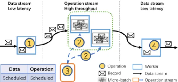
Figure 5 shows the structure diagram of DO, which integrates two paradigms. As we analyzed in Section 2.1, operation stream should be adopted for data burst to avoid long network transmission time and data stream is a better choice for remaining operations to avoid long synchronous time. When data burst occurs, DO automatically sets the heavy-loaded operations to operation stream and other operations to data stream. In this way, we can handle data burst on the heavy-loaded operations with higher throughput while keeping

* * * * * * * * *

Figure 5: Structure diagram of DO

low latency on light-loaded operations. With the help of this dual-paradigm approach, only one framework needs to be deployed to meet both high throughput and low latency at the same time. For example, as shown in Figure 5, stream data should be processed by four operations. Operation 1 produces a data burst, increasing the number of records from 1 to 3. While after Operation 3, the number of records is reduced to 1. In this case, DO chooses operation stream for Operation 2 and Operation 3 to guarantee high throughput, while data stream for Operation 1 and Operation 4 for low latency.

Whenever a data burst occurs, flowing a large number of records through part of operations results in significantly high transmis-sion timettr ans. Take Figure 5 as an example, increasing records transmission between Operations 1, 2, and 3 costs a long latency and hence becomes the bottleneck of latency. To improve the per-formance, DO switches Operation 2 and 3 affected by data burst to operation stream and reduces thettr ansby fixing data to certain

workers. Once the data burst passes, synchronous timetsync of

Operation 2 and 3 becomes the dominant component of latency. Thus, DO switches this part back to data stream which flows records through operations for fast processing records. By switching be-tween operation stream and data stream, network transmission or synchronous time will not become the bottleneck. Without the latency bottleneck, all records are processed fast without waiting

outside the framework, andtoutcan also be significantly reduced,

i.e., improving throughput. Therefore, DO can handle data burst efficiently, and balance throughput and latency.

4.2

Switch Point

As we mentioned above, data burst happens among operations. For example, as shown in Figure 5, data burst occurs from Operation 2. In this section, we introduce our strategy to identify where and when data burst occurs.

As illustrated in Figure 6, we assume that the data arrives at an

average rateV , the average record processing speed of operation

stream isPO, and the average record processing speed of data

stream isPD. Each operation has a buffer queue to store the waiting

data and the queue lengthL represents the data to be processed.

Note that for both operation stream and data stream, the data

burst is directly related to the queue lengthL. A large number of

records over throughput will cause a longer queue length. Therefore, we detect the switch point by finding a queue length which triggers the switching.

In data stream, as we analyzed in Section 2.1, the latency can be calculated by

LatencyD = tou t+ tpr oc+ tt r ans

= 0 +_{P D +}L td t

(4)

wheretdtis the transmission time in data stream.

As for operation stream, the records in the queue are firstly

accumulated as a micro-batch within a time intervalT . Note that

***

the arrival rate of records isV , the micro-batch size after time intervalT is L = V ∗T . Then all these L records in a micro-batch are processed through different operations. The latency of operation stream can be calculated as

LatencyO = tou t+ tw ai t+ ts c hedul e+ tpr oc+ tt r ans

= 0 +T₂ + ts+ L PO +tot =T₂+ ts+ V ∗ T PO +tot (5)

wheretsandtotrefer to the schedule time in operation stream and transmission time in operation stream, respectively.

Under normal circumstances, latency of data stream is lower than operation stream. Only when facing data burst, the latency of data stream will increase and even exceeds the latency of operation stream because of low throughput. So, when the latency of data

stream exceeds operation stream, the queue lengthL can be

calcu-lated in Equation 6. LetK = P D_POandC =T₂+ts+tot−tdt, the switch

queue length can be presented asLswitch= K ∗ (V ∗ T ) + C ∗ PD.

LatencyD > LatencyO =⇒L > P D ∗ [V ∗ T_{PO +}(T

2 + ts+ tot−td t)] =⇒L > K ∗ (V ∗ T ) + C ∗ P D

(6)

That is, if current queue lengthL > Lswitch, data burst starts and this operation should be marked as a switch point. So that the operation stream should be selected on this and subsequent affected operations for the high throughput. Otherwise, ifL < Lswitch, data stream is more suitable due to its low latency.

In order to avoid data arrival rate fluctuations around the thresh-old of the switch point, there is a factorδ, set by user, to calculate

Lup andLdown, as Equation 7 shown. Whenever the length of

records in the waiting queue is higher thanLup or lower than

L_down, the DO will consider to switch the paradigm.

     Lup = (1 + δ ) ∗ Lsw i t c h L_{d ow n} = (1 − δ ) ∗ Lsw i t c h , 0 < δ < 1 (7)

4.3

Switch Range

The switch point identifies when and where the data burst starts, we need to further deicide the range of operations which are affected by data burst.

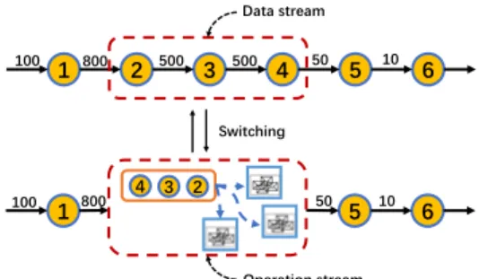
We firstly take Figure 7 as an example. All numbers on the arrow

are the average numbers of records. We useλm to represent the

records magnification ofmth operation. The number of records is

expanded by 8 times after Operation 1, i.e.,λ1= 800/100 = 8. While after Operations 2 and 3, the record number decreases with ratio λ2= 0.625 and λ3= 1, respectively. The number of records shrinks after Operation 4 with ratioλ4= 0.1. We assume that the data burst starts between Operation 1 and 2 (i.e., Operation 2 is the switch point). We set the range of operations whose processing paradigm shall be switched at runtime as {2, 3, 4} because Operations 3 and 4 also need to process a large number of records. Only after Operation 4, the number of records decreases down to the input volume of Operation 1. That isQ4

n=1λn= 0.5 < 1.

That is, the switch range should be skillfully selected according

to the records magnification. Assume that data burst starts atpth

operation, DO looks for the first nextqth operation as the end of the

Figure 7: Switch between operation stream and data stream range with a lower records magnification that satisfies Equation 8.

q

Y

m=p−1

λm < 1 (8)

In our design for choosing switch range, there are two aspects to be considered, also taking Figure 7 as an example. On the one hand, for the start of the range, we do not include Operation 1, because the records produced by Operation 1 can be load balanced by transmitting data to the workers in downstream of operation stream. On the other hand, for the end of the range, we choose minimal range {2, 3, 4} rather than {2, 3, 4, 5} or others because the number of records after Operation 4 is already smaller than the input, so there is no pressure on downstream operations. We use minimum range to achieve maximum benefit.

Similarly, whenever the length of waiting queue in operation stream is lower thanLdown, we can regard that the data burst has passed away and switch back to data stream.

4.4

Switch Steps

To ensure a smooth switch between operation stream and data stream, we propose a switch strategy with low overhead.

We traverse the whole processing topology to generate an opera-tion chain. Without knowledge of the records magnificaopera-tion in each operation, all operations are initially set to data stream to warm up for achieving minimal latency. When data burst occurs, we would like to switch to operation stream for its high throughput. As we have discussed in Section 4.2, data burst is detected via the queue length. Hence at runtime, each worker continuously monitors the queue lengthL. When L is higher than Lupor lower thanLdown, it

will report to DO upon the currentL, DO decides the switch range

and switches the paradigm according to the principle discussed above.

The switch steps of DO adopt a "prepare-switch-run" manner. DO firstly prepares the logic of a new paradigm while the operations to be switched empty the data in them, and then switches the paradigm once the data has been emptied and logic has been prepared. During emptying data, all other operations process data normally and cache them temporarily. After switching, the cached data are sent to the downstream operations. By this way, we can achieve a smooth switch at run-time without data loss.

4.5

Replay-able Uniform Dataset

Since there exist two paradigms in our framework, how to manage data in a uniform way without violating the framework perfor-mance needs to be addressed. To solve this problem, we propose

Replay-able Uniform Dataset (RUD) to unify data management un-der different paradigms.

In general, RUD uses cache to support different data granularity demands in different paradigms. Each operation forms an RUD for each time interval described in Section 4.2. The data is firstly stored at the input cache which separates network transmission and data acquisition. If data stream is selected, the data will be obtained record by record. Otherwise, with operation stream, the data will be obtained as a micro-batch. At the same time, DO takes the worker failure into consideration. If some workers fail, all RUDs at downstream within current time interval will be discarded and all records in previous RUD will be replayed to form the new RUD to downstream. In order to replay records to downstream faster and avoid repeated processing, RUD uses output cache and it only needs to replay records in output cache. If the data within current time interval are processed successfully, all RUDs of this time interval will be deleted. The RUD controller is responsible for replaying or deleting RUDs.

RUD provides an uniform data management interface for the processing paradigm. On the specific implementation methods of RUD, there are two kinds of methods corresponding to operation stream and data stream respectively, as shown in Figure 8.

RUD in data stream is shown in Figure 8(a). Each worker repre-sents a processing node. Worker-k means that the worker is running

thekth operation, i.e., Ok, whileRU Dn-k represents nth RUD in

Worker-k. Processing thread continuously gets records from the input cache. The processed records are transmitted to the down-stream operations with a copy retained in the output cache. Only RUD controller can delete the records in output data cache in case of node failure.

RUD in operation stream is shown in Figure 8(b). Operation stream coordinates many workers to process large numbers of records by scheduling the operations. In this case, Worker-k-p is

thepth worker that begins with kth operation. The basic functions

of RUD in operation stream are the same as data stream, but they are different in the following two aspects: 1) Data chain. Data chain is made up by all batches of data in a RUD as Figure 8(a). Owing to the operation scheduling, operations use data chain to store temp data. Each operation brings an intermediate micro-batch cache to next operation. If any operation fails, all records will be reprocessed from previous temp data. 2) Data balancing. All workers perform the same operation in operation stream, so the data from upstream can be evenly distributed to each node to achieve load balancing.

(a) In data stream (b) In operation stream

Figure 8: Replay-able Uniform Dataset

5

IMPLEMENTATION

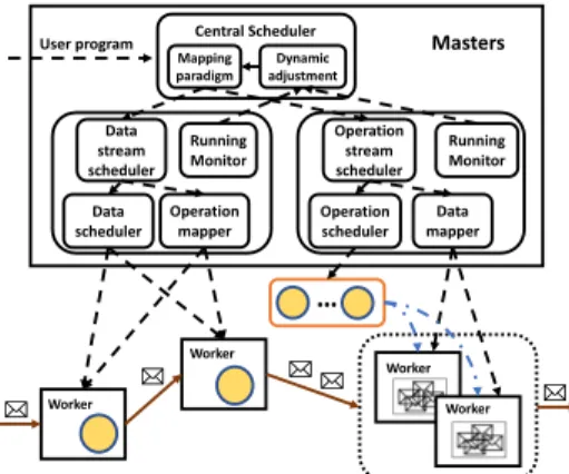
Following the design principles discussed above, we implement a prototype stream processing framework integrating DO as shown in Figure 9. There are three main components, i.e., central scheduler, operation stream, and data stream. We use Spark Streaming engine [28] for operation stream and JStorm [11], the streaming process engine developed by Alibaba, for data stream.

Central scheduler. Central scheduler works as the brain of our prototype framework. We use around 1000 lines of code to realize the central scheduler. As shown in Figure 9, there are two threads for central scheduler as processing logic mapping and run-time switching. Although there are two kinds of paradigms in DO, users only need to submit one processing logic code to central scheduler. When processing logic is submitted, our framework will map the processing logic to two paradigms automatically. The whole procedure is transparent to users.

Operation stream. We write around 2000 lines of codes to mod-ify the scheduler and the block manager in Spark Streaming to support DO for operation stream. The Spark Streaming scheduler connects to the central scheduler and receives processing logic. Note that Spark Streaming submits jobs to Spark core at a fixed time interval, we change the processing logic in next time interval after receiving logic changing instruction from the center scheduler. For Replay-able Uniform Dataset, we apply in practice the RDD lin-eage in Spark Streaming that all RDDs correspond to the temp data cache in Replay-able Uniform Dataset. It will generate an output data batch after completing the job of this time interval and store this batch in block manager of Spark Streaming as the output data cache in Replay-able Uniform Dataset.

Data stream. JStorm is used for implementing data stream. We use around 1500 lines of codes to modify the scheduler and add Replay-able Uniform Dataset in JStorm. When the scheduler re-ceives a paradigm changing signal from central scheduler, it firstly stops sending records from spout, waits until all data in the heavy-loaded operations are processed, then kills or starts workers accord-ing to the assignment of data stream and rebuilds the data pipeline. After all changes complete, the spout starts sending record again. Replay-able Uniform Dataset is added to each processing node for data management.

Mapping paradigm adjustmentDynamic

Data scheduler Running Monitor Data stream scheduler Operation

mapper Operationscheduler

Running Monitor Operation stream scheduler Data mapper Worker Worker Worker Worker … Masters * * * * * Central Scheduler User program

0 1 0 2 0 3 0 4 0 5 0 6 0 0 5 0 0 1 0 0 0 1 5 0 0 2 0 0 0 2 5 0 0 La te nc y (m s) T i m e ( 1 0 s ) S p a r k F l i n k J S t o r m S t o r m T r i d e n t D O

(a) WordCount under 20K events/sec

0 1 0 2 0 3 0 4 0 5 0 6 0 0 5 0 0 1 0 0 0 1 5 0 0 2 0 0 0 2 5 0 0 La te nc y (m s) T i m e ( 1 0 s ) S p a r k F l i n k J S t o r m S t o r m T r i d e n t D O

(b) Grep under 50K events/sec

0 1 0 2 0 3 0 4 0 5 0 6 0 0 5 0 0 1 0 0 0 1 5 0 0 2 0 0 0 2 5 0 0 La te nc y (m s) T i m e ( 1 0 s ) S p a r k F l i n k J S t o r m S t o r m T r i d e n t D O

(c) Yahoo! benchmark under 20K events/sec

0 1 0 2 0 3 0 4 0 5 0 6 0 0 2 0 0 0 0 4 0 0 0 0 6 0 0 0 0 8 0 0 0 0 1 0 0 0 0 0 1 2 0 0 0 0 1 4 0 0 0 0 La te nc y (m s) T i m e ( 1 0 s ) S p a r k F l i n k J S t o r m S t o r m T r i d e n t D O S w i t c h i n g i n D O

(d) WordCount under 50K events/sec

0 1 0 2 0 3 0 4 0 5 0 6 0 0 2 0 0 0 0 4 0 0 0 0 6 0 0 0 0 8 0 0 0 0 1 0 0 0 0 0 La te nc y (m s) T i m e ( 1 0 s ) S p a r k F l i n k J S t o r m S t o r m T r i d e n t D O S w i t c h i n g i n D O

(e) Grep under 80K events/sec

0 1 0 2 0 3 0 4 0 5 0 6 0 0 2 0 0 0 0 4 0 0 0 0 6 0 0 0 0 8 0 0 0 0 1 0 0 0 0 0 1 2 0 0 0 0 La te nc y (m s) T i m e ( 1 0 s ) S p a r k F l i n k J S t o r m S t o r m T r i d e n t D O S w i t c h i n g i n D O

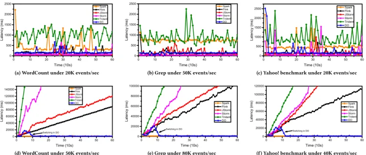
(f) Yahoo! benchmark under 40K events/sec Figure 10: Latency in different benchmark under different data arrival rates

6

EVALUATION

In this section, we evaluate the performance of our prototype frame-work. For comparison, we use Spark Streaming [28] 2.1.0 as oper-ation stream framework, JStorm [11] 2.2.1, Storm [22] 0.10.0, and Flink [12] 1.2.1 as data stream framework and Trident [23] on Storm as variant data stream, which uses micro-batch instead of single record in data stream.

6.1

Setup

Workload. We use WordCount and Grep as the basic stream bench-marks to evaluate latency trends under different data arrival rates in different frameworks. WordCount is CPU-intensive application and Grep is network-intensive application. We also use Yahoo! in-dustrial streaming benchmark [5] to evaluate the dual-paradigm approach with real application. The benchmark is an advertisement application and it has six operations that contain receiver, parse, filter, join, window count, and store back. These steps attempt to probe some common operations performed on stream data.

Experimental Setup. Our evaluations run on a cluster of 6 ma-chines. Each machine is equipped with Intel Xeon E5-2650 2.30GHz CPUs, 128GB memory, and 2TB disks. All machines are intercon-nected with 1Gbps Ethernet cards and run CentOS 7.2.1511. All frameworks use 1 worker for master, 4 workers for processing data, 3 workers for Kafka, 3 workers for Zookeeper, and 1 worker for Redis. The parameter K in DO is set empirically to 0.2.

6.2

Latency under fixed data arrival rate

In this section, we show the latency in different frameworks under different data arrival rates, as shown in Figure 10. It can be observed that, our framework has a low latency under low data arrival rate and a high throughput under high data arrival rate. In all settings, the advantage of DO can be observed.

The results of WordCount are shown in Figure 10 (a) and (d). Under data arrival rate of 20K events/sec, all frameworks show a stable latency below seconds. With a small number of records, data stream frameworks have a lower latency than operation stream or variant data stream. The reason is that records are processed one by one and then written back once processed. Our DO framework also keeps a competitively low latency by setting all operations to data stream. As for operation stream, waiting time becomes the bottleneck as discussed in Section 6.4, leading to a higher latency. A noticeable finding is that the performance of our framework is slightly higher than JStorm and Storm because the Kafka receiver in our framework synchronizes each 50ms.

When data arrival rate rises up to 50K events/sec in WordCount, the latencies of all data stream frameworks keep increasing. The reason is that the data arrival rate is higher than the throughput and causes a backpressure to lower the intake data rate. That is to say, more records have to wait outside the framework, results in a higher outside waiting time as well as higher latency. For operation stream, e.g., Spark Streaming, it puts data at a fixed node to avoid large data transmission through network. Our framework integrates these two paradigms and achieves a high throughput for operations with a large number of records and a low latency for operations with a small number of records at the same time. By setting operations to different processing paradigms, operation stream will not be applied to all operations in our framework. As a result, records are transmitted to data stream operations once completed in operation stream to get a lower latency.

Similar trends can be observed in Grep and Yahoo! industry bench-mark as shown in Figure 10 (b), (e), (c), and (f). The latency of data stream keeps stable under a low data arrival rate (i.e., 50K in Grep or 20K in Yahoo! industry benchmark) while increases under a high data arrival rate (i.e., 80K in Grep or 40K in Yahoo! industry bench-mark). In contrast, operation stream and DO keep a stable latency under both data arrival rates. Nevertheless, no matter using which

2 0 0 0 0 3 0 0 0 0 4 0 0 0 0 5 0 0 0 0 6 0 0 0 0 7 0 0 0 0 8 0 0 0 0 0 1 0 0 2 0 0 3 0 0 4 0 0 5 0 0 6 0 0 7 0 0 0 5 0 0 0 0 1 0 0 0 0 0 1 5 0 0 0 0 Da ta a rri va l r at e (e ve nt s/ se c) La te nc y (m s) T i m e ( s ) F l i n k J s t o r m S p a r k S t o r m T r i d e n t D O

Figure 11: Latency of different frameworks under data burst benchmark and under what arrival rate, the advantages of our DO can always be observed.

6.3

Latency under data burst

We use the Yahoo! industry benchmark and simulate the data burst to indicate the processing capacity of different frameworks and recovery time as shown in Figure 11.

We can see that the latencies of all frameworks vary with time and data arrival rate. With a low data arrival rate, all frameworks process records with a low latency. Once data burst occurs, the latency of our framework jumps to a relatively high level compared to other frameworks because of the paradigm switch. That is our framework successfully detects this data burst and switches the pro-cessing paradigm of heavy-loaded operations to operation stream. This makes a peak latency, but return to a low level very soon once the switch is done. As shown in Figure 11, our framework can handle data burst efficiently after switching. Spark Streaming can keep a stable latency at first data burst due to its higher throughput than this data arrival rate. The latencies of other frameworks keep increasing during the data burst with different increasing speeds and decrease when data burst ends. Flink has a better performance than other data stream frameworks. At the second data burst, the latency of our framework firstly rises and then remains stable while the latencies of other frameworks keep increasing. A conclusion can be drawn that our framework handles data burst better than other frameworks.

6.4

Latency per component

In this section, we use Yahoo! industry benchmark to evaluate the different components of latency in data stream, operation stream, variant data stream, and DO. We use JStorm, Spark Streaming, Trident, and our framework for different processing paradigms, respectively. The results are shown in Table 1 and Table 2. Table 1: Latency components of frameworks in low data ar-rival rate of 4K events/sec

JStorm Spark Trident DO

outside wait 0 0 0 0

process 0.38ms 0.07ms 0.04ms 0.45ms

wait 0 285ms 184ms 0

schedule 0 24ms 0 0

network transmission 41ms 22ms 95ms 61ms

We can observe from Table 1 that data stream has a lower la-tency compared to others in a low data arrival rate and network transmission is the dominant component of the latency, accounting for up to 99.1%. In contrast, network transmission is only 6.6% in operation stream latency. That is because the network transmission occurs only in the shuffle phase and the records are transmitted as a micro-batch. In this case, waiting and scheduling times become the bottleneck. A record must use 4071x more time than the processing time to wait for other records in the same micro-batch. Meanwhile, scheduling time is 342x higher than processing time. For Trident, waiting and network transmission are both the main factors con-tributing to the latency, up to 65.9% and 34.0%, respectively. Our framework keeps whole processing topology into data stream due to low data arrival rate. So the latency component of our framework is almost the same as JStorm and has no time wasted on waiting or scheduling.

Table 2: Latency components of frameworks in high data ar-rival rate of 40K events/sec

JStorm Spark Trident DO

outside wait increase 0 increase 0

process 0.39ms 0.02ms 0.03ms 0.36ms

wait 0 713ms 946ms 554ms

schedule 0 39ms 0 12ms

network transmission 1533ms 44ms 459ms 220ms

Next, Table 2 shows the latency components when data arrival rate is up to 40K event/sec. Compared with Table 1, the record processing times in four frameworks are almost the same, because the processing logic is the same, but other latency components vary a lot. In data stream, the large amount of records causes a high pressure on the network, making a long network transmission time as 37x higher than before. What is worse, the data arrival rate is higher than the maximum throughput, making outside wait time increases. In operation stream, when the number of records increases, the record needs more time to wait for other records of the same micro-batch, leading to a 2.5x higher waiting time. Trident is impacted by both waiting and network transmission. The latency of waiting is 5.1x higher and network transmission time is 4.8x higher than before. With dual-paradigm approach, our framework switches heavy-loaded operations into operation stream, thus introduces waiting time and scheduling time. But the waiting time and scheduling time are both lower than Spark Streaming. Switching also causes lower network transmission time than data stream. What is more, the whole latency keeps stable and no data is blocked outside the framework, i.e., no outside wait time.

6.5

Latency per operation

Now, we use Yahoo! industry benchmark to evaluate latency at oper-ation level to indicate the inner details of DO. Figure 12 illustrates inner state of DO under different data arrival rates, in particular, the latency at operation level compared to JStorm and Spark.

At a low data arrival rate of 20K events/sec, as shown in Fig-ure 12(a), our framework sets all operations to data stream to achieve a similar performance as JStorm. Due to the its micro-batch processing manner, Spark Streaming has a higher latency.

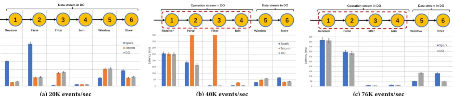
(a) 20K events/sec (b) 40K events/sec (c) 76K events/sec

Figure 12: Latency per operation under different data arrival rates. The latency of each operation is defined as time interval from the end of the previous operation to the end of the current operation, including network transmission. JStorm suffers frequently backpressure at 76K events/sec, makes a fluctuant latency, so it does not shown in (c).

The reason why latencies of Operations 3 and 5 in our framework and JStorm are higher than that of Spark Streaming is that these two operations and their upstream operations are allocated to different nodes. This causes data transmission between the nodes with a higher latency. When data arrival rate is up to 40K events/sec as Figure 12(b), JStorm is unstable and uses backpressure to control network transmission. The latencies of Operation 2 and 3 in JStorm are much higher than that of Spark Streaming because the records in JStorm are waiting to be processed at the buffer queue in Operation 2 and 3. At this time, our framework switches the paradigm of the first four operations to operation stream for higher throughput and lower latency. At Operation 5, our framework has a higher latency than Spark Streaming because of the data transmission of Operation 4. But the number of records after Operation 4 is lower than the throughput of data stream. So our framework keeps Operation 5 and 6 in data stream.

Then, we increase the data arrival rate to 76K events/sec, as shown in Figure 12(c). Compared to 40K events/sec, we find that latency of each operation rises in all frameworks. Our framework still puts the first four operations to operation stream and keeps last two in data stream. This is also the reason why the throughput of our framework is higher than Spark Streaming, as illustrated in Section 6.6. For Spark Streaming, it always completes all six opera-tions on the present micro-batch before next. Under the data arrival rate of 76K events/sec, the whole latency is higher than the batch interval of Spark Streaming as 1 second. So next micro-batch must wait outside, causing an increase in the outside wait time as well as a higher latency. Meanwhile in our framework, operation stream only needs to process first four operations and then transmits data to data stream. Total latency of first four operations is lower than the batch interval, i.e., 1 second. Meanwhile, the number of records after Operation 4 decreases significantly and does not cause data burst to downstream data stream, that makes the whole latency in a stable state. All these strategies result our framework in a higher throughput and a lower latency than operation stream.

6.6

Throughput

In this section, we evaluate the maximum throughput of each frame-work to explore their processing capacity in Figure 13. Different benchmarks will cause different throughputs as show in Figure 10 (b) and (d), therefore we use Yahoo! industry benchmark to indi-cate their throughputs in the real environment. Storm, JStorm,

0 1 0 0 0 0 2 0 0 0 0 3 0 0 0 0 4 0 0 0 0 5 0 0 0 0 6 0 0 0 0 7 0 0 0 0 8 0 0 0 0 S t o r m T r i d e n t J s t o r m F l i n k S p a r k D O Th ro ug hp ut (e ve nt s/ se c)

Figure 13: Throughput of different frameworks and Trident have relatively low throughput compared to others. The reason is that network transmission becomes the bottleneck when facing a large number of records. These data trigger backpres-sure, resulting in data waiting outside frameworks and thus a low throughput. Flink uses a scheduling method that integrates opera-tions for direct data association into a single operation to reduce the impact of network transmission and improve the throughput. Spark Streaming uses micro-batch processing to get a higher throughput. Different from them, our framework uses micro-batch processing only at heavy-loaded operations, resulting in a higher throughput than Spark Streaming, as explained in Section 6.5. As a result, the throughput of our framework is 1.14x higher than Spark Streaming, 2.1x higher than Flink, 2.9x, 3.0x, and 3.2x higher than Trident, JStorm, and Storm respectively.

7

RELATED WORK

Data stream. The representative frameworks of data stream are S4 [17], MillWheel [1], Naiad [16], Samza [19], Storm [22], Flink [12], and Heron [14]. Data stream suffers of a noticeable perfor-mance loss when facing large number of records (i.e., data bursts). Consequently, many research works have focused on handling data bursts, they can be grouped into two categories. First is online or offline operation scheduling to reduce network transmission time [2, 3, 13, 27]. But those methods will cause data skew as some nodes process large data volume and transmit smaller data volume to other nodes. In contrast, DO uses operation stream which can balance large data volume to all nodes. Second is sacrificing the accuracy to get a higher latency, i.e., approximation [4, 10, 15]. DO can provide accurate result even when data burst occurs.

Operation stream. Another idea for stream processing is to divide stream data into micro-batches before processing them, such as Spark Streaming [28], Nova [18], Incoop [6], and MapReduce Online [7]. Usually they have a high throughput due to batch pro-cessing. In order to reduce the latency of operation stream, different methods are proposed. Given that batch sizes can greatly impact the latency, Christopher Olston et al. [8] propose a control algo-rithm that automatically adapts the batch size to get a low latency, but it still uses micro-batches and the latency is higher than data stream. DO totally uses data stream to get a lower latency. The most recent work, Drizzle [24], targets reducing the latency in operation stream by reducing the latency of scheduling in different parts of a micro-batch. However, it suffers a performance loss under data bursts as it does not consider the time of waiting other records to be processed.

8

CONCLUSION

In this paper, we propose DO, a fine-grained dual-paradigm ap-proach for stream data processing. It embraces a method at opera-tion level to detect data bursts, identify the main operaopera-tions with data burst, and divide the whole stream processing topology into several parts with different processing paradigms. Furthermore, we propose a Replay-able Uniform Dataset to unify data management in different paradigms. Based on our design, a prototype stream processing framework is implemented to adopt DO. Experimental results demonstrate that DO achieves a comparable performance on latency to data stream and achieves 5x speedup over operation stream under low stream data sizes. DO also outperforms operation stream on throughput by 1.14x and outperforms data stream on throughput by around 2.1x to 3.2x under data bursts.

ACKNOWLEDGEMENT

This work is supported by National Key Research and Development Program under Grant 2018YFB1003600, the ANR KerStream project (ANR-16- CE25-0014-01), Science and Technology Planning Project of Guangdong Province in China under grant 2016B030305002, and Pre-research Project of Beifang under grant FFZ-1601.

REFERENCES

[1] Tyler Akidau, Alex Balikov, Kaya Bekiroğlu, Slava Chernyak, Josh Haberman, Reuven Lax, Sam McVeety, Daniel Mills, Paul Nordstrom, and Sam Whittle. 2013. MillWheel: Fault-tolerant Stream Processing at Internet Scale. Proceedings of the VLDB Endowment. 6, 11 (Aug. 2013), 1033–1044.

[2] Leonardo Aniello, Roberto Baldoni, and Leonardo Querzoni. 2013. Adaptive On-line Scheduling in Storm. In Proceedings of the 7th ACM International Conference on Distributed Event-based Systems (DEBS ’13). ACM, 207–218.

[3] Brian Babcock, Shivnath Babu, Rajeev Motwani, and Mayur Datar. 2003. Chain: Operator Scheduling for Memory Minimization in Data Stream Systems. In Proceedings of the 2003 ACM SIGMOD International Conference on Management of Data (SIGMOD ’03). ACM, 253–264.

[4] Brian Babcock, Mayur Datar, and Rajeev Motwani. 2003. Load shedding tech-niques for data stream systems. In Proceedings of the 2003 Management and Processing of Data Streams Workshop (MPDS ’03), Vol. 577. ACM.

[5] Yahoo! Streaming Benchmark. 2015. https://yahooeng.tumblr.com/post/ 135321837876/

[6] Pramod Bhatotia, Alexander Wieder, Rodrigo Rodrigues, Umut A. Acar, and Rafael Pasquin. 2011. Incoop: MapReduce for Incremental Computations. In Proceedings of the 2011 ACM Symposium on Cloud Computing (SOCC ’11). ACM, Article 7, 14 pages.

[7] Tyson Condie, Neil Conway, Peter Alvaro, Joseph M. Hellerstein, Khaled Elmele-egy, and Russell Sears. 2010. MapReduce Online. In Proceedings of the 7th USENIX Symposium on Networked Systems Design and Implementation (NSDI ’10). USENIX, 313–328.

[8] Tathagata Das, Yuan Zhong, Ion Stoica, and Scott Shenker. 2014. Adaptive Stream Processing Using Dynamic Batch Sizing. In Proceedings of the 2014 ACM Symposium on Cloud Computing (SOCC ’14). ACM, Article 16, 13 pages. [9] Structured Streaming Programming Guide. 2018. http://spark.apache.org/docs/

latest/structured-streaming-programming-guide.html

[10] Martin Hirzel, Robert Soulé, Scott Schneider, Buğra Gedik, and Robert Grimm. 2014. A Catalog of Stream Processing Optimizations. ACM Comput. Surv. 46, 4, Article 46 (March 2014), 34 pages.

[11] JStorm. 2015. http://jstorm.io/

[12] Asterios Katsifodimos and Sebastian Schelter. 2016. Apache Flink: Stream Ana-lytics at Scale. In Proceedings of the 2016 IEEE International Conference on Cloud Engineering Workshop (IC2EW ’16). IEEE, 193–193.

[13] Wilhelm Kleiminger, Evangelia Kalyvianaki, and Peter Pietzuch. 2011. Balancing load in stream processing with the cloud. In Proceedings of the 27th IEEE Interna-tional Conference on Data Engineering Workshops (ICDEW ’11). IEEE, 16–21. [14] Sanjeev Kulkarni, Nikunj Bhagat, Maosong Fu, Vikas Kedigehalli, Christopher

Kellogg, Sailesh Mittal, Jignesh M. Patel, Karthik Ramasamy, and Siddarth Taneja. 2015. Twitter Heron: Stream Processing at Scale. In Proceedings of the 2015 ACM SIGMOD International Conference on Management of Data (SIGMOD ’15). ACM, 239–250.

[15] Julie Letchner, Christopher Ré, Magdalena Balazinska, and Matthai Philipose. 2010. Approximation trade-offs in Markovian stream processing: An empirical study. In Proceedings of the 26th IEEE International Conference on Data Engineering (ICDE ’10). IEEE, 936–939.

[16] Derek G. Murray, Frank McSherry, Rebecca Isaacs, Michael Isard, Paul Barham, and Martín Abadi. 2013. Naiad: A Timely Dataflow System. In Proceedings of the 24th ACM Symposium on Operating Systems Principles (SOSP ’13). ACM, 439–455. [17] Leonardo Neumeyer, Bruce Robbins, Anish Nair, and Anand Kesari. 2010. S4:

Dis-tributed Stream Computing Platform. In Proceedings of the 2010 IEEE International Conference on Data Mining Workshops (ICDMW ’10). IEEE, 170–177. [18] Christopher Olston, Greg Chiou, Laukik Chitnis, Francis Liu, Yiping Han, Mattias

Larsson, Andreas Neumann, Vellanki B.N. Rao, Vijayanand Sankarasubramanian, Siddharth Seth, Chao Tian, Topher ZiCornell, and Xiaodan Wang. 2011. Nova: Continuous Pig/Hadoop Workflows. In Proceedings of the 2011 ACM SIGMOD International Conference on Management of Data (SIGMOD ’11). ACM, 1081–1090. [19] Samza. 2015. http://samza.apache.org/

[20] Michael Stonebraker, Uˇgur Çetintemel, and Stan Zdonik. 2005. The 8 Require-ments of Real-time Stream Processing. SIGMOD Rec. 34, 4 (Dec. 2005), 42–47. [21] Jaspar Subhlok and Gary Vondran. 1996. Optimal Latency-throughput Tradeoffs

for Data Parallel Pipelines. In Proceedings of the 8th Annual ACM Symposium on Parallel Algorithms and Architectures (SPAA ’96). ACM, 62–71.

[22] Ankit Toshniwal, Siddarth Taneja, Amit Shukla, Karthik Ramasamy, Jignesh M. Patel, Sanjeev Kulkarni, Jason Jackson, Krishna Gade, Maosong Fu, Jake Donham, Nikunj Bhagat, Sailesh Mittal, and Dmitriy Ryaboy. 2014. Storm@twitter. In Proceedings of the 2014 ACM SIGMOD International Conference on Management of Data (SIGMOD ’14). ACM, 147–156.

[23] Trident. 2015. http://storm.apache.org/releases/1.1.0/Trident-tutorial.html [24] Shivaram Venkataraman, Aurojit Panda, Kay Ousterhout, Michael Armbrust,

Ali Ghodsi, Michael J. Franklin, Benjamin Recht, and Ion Stoica. 2017. Drizzle: Fast and Adaptable Stream Processing at Scale. In Proceedings of the 26th ACM Symposium on Operating Systems Principles (SOSP ’17). ACM, 374–389. [25] Naga Vydyanathan, Umit Catalyurek, Tahsin Kurc, Ponnuswamy Sadayappan,

and Joel Saltz. 2011. Optimizing latency and throughput of application workflows on clusters. Parallel Comput. 37, 10 (2011), 694 – 712.

[26] Walter Willinger, Murad S. Taqqu, and Ashok Erramilli. 1996. A Bibliographical Guide to Self-Similar Traffic and Performance Modeling for Modern High-Speed Networks. Stochastic Networks Theory and Applications (1996), 339–366. [27] Jielong Xu, Zhenhua Chen, Jian Tang, and Sen Su. 2014. T-Storm: Traffic-Aware

Online Scheduling in Storm. In Proceedings of the 34th IEEE International Confer-ence on Distributed Computing Systems (ICDCS ’14). IEEE, 535–544.

[28] Matei Zaharia, Tathagata Das, Haoyuan Li, Timothy Hunter, Scott Shenker, and Ion Stoica. 2013. Discretized Streams: Fault-tolerant Streaming Computation at Scale. In Proceedings of the 24th ACM Symposium on Operating Systems Principles (SOSP ’13). ACM, 423–438.