io3,
Université de Montréal
Weighted Finite-$tate Transducers in Speech Recognition:
A Compaction Algorithm for Non-Determinizable
Transducers
par
Shouwen Zhang
Département d’informatique et de recherche opérationnelle
Faculté des arts et des sciences
Mémoire présenté à la faculté des études supérieures
en vue de l’obtention du grade de
Maîtrise ès sciences (M.Sc.)
en informatique
Décembre, 2002
r
r
î —,
J
(JUniversité
de Montréal
Direction des bibliothèques
AVIS
L’auteur a autorisé l’Université de Montréal à reproduire et diffuser, en totalité ou en partie, par quelque moyen que ce soit et sur quelque support que ce soit, et exclusivement à des fins non lucratives d’enseignement et de recherche, des copies de ce mémoire ou de cette thèse.
L’auteur et les coauteurs le cas échéant conservent la propriété du droit d’auteur et des droits moraux qui protègent ce document. Ni la thèse ou le mémoire, ni des extraits substantiels de ce document, ne doivent être imprimés ou autrement reproduits sans l’autorisation de l’auteur.
Afin de se conformer à la Loi canadienne sur la protection des renseignements personnels, quelques formulaires secondaires, coordonnées ou signatures intégrées au texte ont pu être enlevés de ce document. Bien que cela ait pu affecter la pagination, il n’y a aucun contenu manquant.
NOTICE
The author of this thesis or dissertation has granted a nonexclusive license allowing Université de Montréal to reproduce and publish the document, in part or in whole, and in any format, solely for noncommercial educational and research purposes.
The author and co-authors if applicable retain copyright ownership and moral rights in this document. Neither the whole thesis or dissertation, nor substantial extracts from it, may be printed or otherwise reproduced without the author’s permission.
In compliance with the Canadian Privacy Act some supporting forms, contact information or signatures may have been removed from the document. While this may affect the document page count, it does not represent any loss of content from the document.
Université de Montréal
Faculté des études supérieures
Ce mémoire intitulé:
Weighted Finite-State Transducers in Speech
Recognition: A Compaction Algorithm for Non
Determinizable Transducers
Présenté par:
Shouwen Zhang
A été évalué par un jury composé des personnes suivantes:
Langlais, Philippe
Président-rapporteur
Aïmeur, Esma
Directeur de recherche
Dumouchel, Pierre
Codirecteur
Poulin, Pierre
Membre du jury
Résumé
Ma thèse donne un aperçu de l’utilisation des transducteurs à états finis pondérés dans le domaine de la reconnaissance de la parole. La théorie des transducteurs permet une manipulation efficace des modèles de langage humain dans les systèmes de reconnaissance de la parole en représentant, de façon générale et naturelle, les différentes composantes du réseau de connaissances. Ce réseau est construit efficacement grâce aux opérations générales qui permettent de combiner, d’optimiser et d’élaguer des transducteurs. La plupart des opérations applicables aux transducteurs ainsi que leur utilisation en reconnaissance de la parole sont décrites en détail. Ensuite, un algorithme permettant de “ compacter “ les transducteurs non-déterminisables est développé et testé
sur plusieurs transducteurs, montrant ainsi son efficacité à diminuer leur taille.
Mots clés: transducteurs à états finis pondérés, reconnaissance de la parole, réseau de connaissances, compactage, déterminisation
Abstract
My thesis surveys the weighted finite-state transducers (WF$Ts) approach to speech recognition. WFSTs provide a powerful method for manipulating models of human language in automatic speech recognition systems due to their common and natural representations for each component of speech recognition network. General transducer operations can combine, optimize, search and prune the recognition network efficiently. The most important transducer operations and their applications in speech recognition are described in detail. Then a transducer compaction algorithm for non-determinizable transducers is developed and some test resuits show its effectivcness in reducing the size ofthe transducers.
Keywords: weighted finite-state transducers, speech recognition, recognition network compaction, determinization.
TABLE 0F CONTENTS .
LISI 0F FIGURES iv
1. Introduction 1
1.1 Continuous Speech Recognition 1
1.2 f inite-State Transducers in Speech Recognition 2
1.3 Contribution 3
1.4 Thesis Organization 4
2. Introduction of Speech Recognition and the Finite-State Transducers 6
2.1 Speech Rcognition 6
2.1.1. Introduction 6
2.1.2. Generative Mode! for Speech Recognition 7
2.1.2.1. Acoustic Model $ 2.1.2.2 Pronunciation Model 9 2.1.3 Language Model 9 2.1.4Decoding 10 2.2 f inite-State Devices 11 2.2.1. f inite-State Automata 13 2.2.1.1 Definitions 13 2.2.1.2. ClosureProperties 14
2.2.2. Mathematical Foundations for Finite-State Transducers 15
2.2.2.1. $emiring 15
2.2.2.2. Power Series 16
2.2.2.3. Weighted Transductions and Languages 17
2.2.3. finite-State Transducers 17
2.2.3.1. Definitions 17
2.2.4. Sequential Transducers 18
2.2.5. Subsequential and p-Subsequential Transducers 19
2.2.6. String-to-Weight Transducers/Weighted Acceptors 22
2.2.6.1 Weighted Finite-State Acceptors (Wf SAs) 22
2.2.7. Weighted Transducers . 25
2.2.7.1 General Weighted Transducers 25
2.2.7.2. Sequential Weighted Transducers 26
3. Weighted Acceptor and Iransducer Operations 28
3.1. Basic Operations 28
3.2. Composition 29
3.2.1. Theoretical Definition and Operation 29
3.2.2. Composition Algorithm 31
3.2.2.1 -free composition 31
3.2.2.2 General case composition 32
3.2.2.3 Complexity 35
3.3. Determinization 35
3.3.1. Determinization Algorithm for Power Series 36 3.3.2. Weighted Transducer Determinization Algorithm 40 3.3.2.1 Pseudocode and Description of WT_determinization Algorithm 41 3.3.2.2 A Proofofthe WT determinization Algorithm 49 3.3.2.3 Space and Complexity ofthe WT_determinization Algoritbm 50
3.4. Minimization 51
4. Weighted Finite-State Transducer Applications in Speech Recognition 53
4.1 Network Components 53 4.1.1. Transducer O 53 4.1.2 TransducerH 54 4.1.1. Transducer C 55 4.1.2 TransducerL 56 4.1.1. Transducer G 56 4.2 Network Combination 57 4.3. Network Standardization 59 4.3.1. Determinization 59 4.3.2. Minimization 61
5. The Compaction of Finite-State Transducers. 63
5.1 Transducer Compaction 63
5.2 The Automata Determinization 63
5.2.1. The Automata Determinization Algorithm 64
5.2.2. The Complexity ofthe Automata Determinization Algorithm 65
5.3 Weight Pushing 66
5.3.1. Reweighting 66
5.3.2. Weight Pushing Pseudocode 69
5.4 The Automata Minimization 71
5.4.1. Partitioning 71
5.4.2. Applications of Partitioning Algorithm 72
5.4.3. The Automata Minimization Algorithrn 74
5.5 The Complexity ofTransducer Compaction 76
5.6 Transducer Compaction in Speech Recognition 77
6. The Experimental Tests of the Transducer Compaction Algorithm 7$
6.1 Test Components 78
6.2 Experimental Tests 79
6.2.1 AUPELf Task 79
6.2.2 Test and Resuit 79
7. Conclusion $2
7.1 Review ofthe Work $2
7.2 future Work 84
LIST 0F FIGURES
1.1 Speech Recognition Stages 1
2.1 HMM with 3 emitting states $
2.2 Recognition cascade 10
2.3 A finite-state automaton example 14
2.4 A 2-subsequential transducer example 19
2.5 A weighted finite-state acceptor 22
2.6 A weighted transducer example 26
3.1 Example of -free transducer composition 30
3.2 Pseudocode ofthe &-ftee composition 32
3.3 Transducers withg labels 33
3.4 Composition with marked g’s 33
3.5 Composition Output 33
3.6 Composition filter 34
3.7 Algorithm for the determinization ofa weighted acceptor T1 defined on the semfring
(R+ u {cc}, mm, +, cia, 0) 36
3.8 Algorithm for the determinization ofa weighted transducer T1 defined on the
semiring
(
u {co}, A, •, co, g)x (R+ u {cc}, mm, +, co, 0) 413.9 47
3.10 48
3.11 Weighted acceptor A 52
3.12 weighted acceptor A1 obtained by pushing from A in the tropical semiring 52
3.13 Weighted acceptorA2 obtained by minimizingAi 52
4.1 Weighted accepetor for acoustic observation 54
4.2 A HMM transducer for a context-dependent model phone b 54
4.3 Context-dependent triphone transducer 55
4.4 A word mode! as weighted transducer 56
4.5 A toy pronunciation lexicon as transducer L 56
4.6 A toy language mode! as weighted transducer 57
5.1 The automata determinization algorithm. 64
5.2 Weighted acceptorAi 67
5.3 Weighted acceptor A2 obtained bypushing from A1 in the tropical semiring 6$ 5.4 Weighted acceptor A3 obtained bypushing from A1 in the 10g semiring 6$
5.5 Generic single-source shortest-distance algorithm 69
5.6 Partitioning algorithm 72
5.7 The automata minimization algorithm 74
Acknowledgement
I would like to express my hearty appreciation to my supervisor Esma Aïmeur for her inspiring guidance toward a research work. Her encouragement and advice are the most valuable experience in my career of study.
I am grateful to my co-supervisor Pierre Dumouchel for his kindness in supporting me to get the opportunity to do my research work in CRIM and interesting me in the area of speech recognition. His support also provided me with the opportunity of preparing my future career.
I am also grateful to Gilles Boulianne, Patrick Cardinal and Jun Qiu for their comments and help in doing my research in CRIM.
Chapter 1
Introduction
Continuous Speech Recognition (CSR) is sufficiently mature that a variety of real world applications are now possible including large vocabulary transcription and interactive spoken dialogue. Speech Recognition has been an active field of study since the beginning of the 5OEs. Great progress has been made, especially since the 7Os, using statisticaÏ modeling approaches with Hidden Markov Models (HMMs) and is nowadays regarded as one ofthe promising technologies ofthe future.
1.1 Continuous Speech Recognition
Speech recognition systems generally assume that the speech signal is a realization of some message encoded as a sequence of one or more symbols [42]. To recognize the underlying symbol sequence given a spoken utterance, the continuous speech waveform is first converted to a sequence of equally spaced discrete parameter vectors. These speech vectors are then transduced into messages by several stages [42]. Each stage can be represented as a component of speech recognition network. Figure 1.1 illustrates the stages for CSR. The speech vectors are first transduced into phones, the minimal units of speech sound in a language that cari serve to distinguish one word from another. The phones are then transduced into syllables, the phonological units which are sometimes thought to interpose between the phones and the word level. Afier that, words are formed by concatenating the syllables and then the recognized sentences are composed with these words.
Obser- Speech Phones $ylla- Words Senten
vation Vectors bles ces
The statistical approach assumes that the CSR problem is a search problem which is to find the “best” word sentences with the largest probability for a given an utterance. Usually cross-word modeling is used between transduction stages for high-accuracy recognition. In other words, each word can be expanded in a sequence of context dependent HMM states, conditioned on the neighboring words. The recognized words are then determined by the most probable state sequence.
However, currently the major concems of CSR are the time and space efficiency, especially for Large Vocabulary Continuous Speech Recognition (LVCSR). Indeed, one of the trends which clearly corne out of the new studies of LVCSR is a large increase in the size of data. The effect of the size increase on time and space efficiency is probably the main computational problem one needs to face in LVCSR.
1.2 Finite-State Transducers in Speech Recognition
In the previous section, we have introduced that the spoken utterances are recognized via some transduction stages. Normally, a transduction stage in CSR is modeled by a finite state device, which is a string-to-string (like the dictionary), string-to-weight (like the language model), or string-to-string/weight transducer (like the hidden Markov models). Each finite-state device in a transduction stage stands for a component of a recognition network.
The application of finite-state transducers in natural language and speech processing is a popular research area [6, 17, 18, 19, 25, 29J. This area is attracting a great deal of attention in the research in Speech Recognition because each component of the recognition network can be represented by transducers (for example, the hidden Markov models) and then these representations can be flexibly and efficiently combined and optimized by transducer operations. The use of finite-state transducers in speech recognition is mainly motivated by considerations of time and space efficiency. Time efficiency is usually achieved by using sequential/deterministic transducers. The output of sequential transducers depends, in general linearly, only on the input size and can therefore be considered as optimal from this point of view. Space efficiency is achieved with transducer minimization algoritbms [20] for sequential transducers.
The important research topics on the finite-state transducers are their mathematically well-defined operations that can generalize and efficiently implement the common methods for combining and optimizing probabilistic models in speech processing. furthermore, new optimization opportunities arise from viewing ail symbolic levels of CSR modeling as weighted transducers [22, 29]. Thus, weighted finite-state transducers define a common ftamework with shared algorithms for the representation and use of the models in speech recognition.
The important finite-state transducer operations are composition, determinization, and minimization. The composition can combine ail levels of the CSR network into a single integrated network in a convenient, efficient, and general manner. The determinization algorithms try to construct an equivalent sequential transducer of a weighted transducer. Instead of the original non-sequential transducer, this sequential transducer dramatically increases the searching speed in Speech Recognition process. The mnning time of sequential transducers for specific input depends linearly only on the size of the input. In most cases the determinization of transducer flot only increases time efficiency but also space efficiency. The minimization can reduce the size of the CSR network and thus increase the space efficiency.
1.3 Contribution
The main contribution of my research is the presentation of a transducer compaction operation which can be applied on non-determinizable transducers to reduce the size of the transducers. It is useful in CSR to increase time and space efficiency when the recognition network is represented by weighted finite-state transducers. Moreover, the implementation of the transducer compaction operation we have done in Centre de Recherche Informatique de Montréal (CRIM) will be part of the tools for the speech recognizer of CRIM.
1.4 Thesis Organization
The purpose ofthis thesis is to survey the weighted transducers in speech recognition and then present a transducer compaction algorithm which can be applied on non determinizable transducers to reduce their size.
First, in Chapter 2, we give a review on statistical speech recognition and finite-state devices. We describe the CSR problem as a decoding problem to find the word sentences with the largest probability. The decoding is done with appropriate search strategy on the recognition network formed by its components which are an acoustic model, a context dependency phone mode!, a pronunciation !exiconldictionary and a language mode! in cascade. Then, we give an extended description of some finite-state devices, these are automata, string-to-string transducers, weighted acceptors, and weighted transducers. We first describe the definitions and properties of automata. Next we consider the case of string-to-string transducers. These transducers have been successful!y used in the representation of large-scale dictionaries. We describe the theoretica! bases for the use of these transducers. In particular, we recali ciassical theorems and give new ones characterizing these transducers. We then consider the case of sequentiai weighted acceptors and weighted transducers. These transducers appear very interesting in speech recognition. Language models are represented by weighted acceptors and HMMs are represented by weighted transducers. We give new theorems extending the characterizations known for usua! transducers to these transducers. We a!so characterize the unambiguous transducers admitting determinization.
In Chapter 3, we describe some transducer operations. We briefly describe some basic transducer operations such as union, concatenation, Kleene closure, projection, best path, N-best path, pruning, topologica! sort, reversai, E-removal, and inversion. Then we give a detai!ed description of composition, determinization, and minimization. We first formally define the composition operation. We also describe the composition a!goritbm for E-free transducers, then its extension for generai case composition is given. Composition operation can constnict complex transducers from simpler ones and combine different levels of representation in speech recognition. furthermore we define
an aÏgorithm for determinizing weighted acceptors, then its extension for determinizing weighted transducers is given, and its correctness is proved. We also briefly describe the minimization of sequential transducers which has a compÏexity equivalent to that of classical automata minimization.
In Chapter 4, we discuss the application of transducers in speech recognition. Each component of a recognition network can be represented by transducers. Then the transducers in network cascade are combined using the composition operation. Finally the network is optimized via determinization and minimization during composition.
In Chapter 5, we present a transducer compaction algorithm. It can apply on non determinizable transducers to reduce their size. This operation includes five steps: weight pushing, encoding, determinization, minimization, and decoding. We first give the automata determinization algorithm and then the weight pushing algorithm. The automata determinization algorithm is the classical powerset construction algorithm which can transform any non-deterministic finite automaton (NFA) into an equivalent deterministic finite automaton (DfA). The weight pushing algorithm, which is similar to a generic single source shortest distance algorithm, is to push the weight towards the initial state as mucli as possible. Then we give the classical automata minimization algorithm which can minimize the size of the automata. The transducer compaction operation is just a combination of these algorithms in appropriate order. At last we describe the applications of the transducer compaction operation in speech recognition.
In Chapter 6, we describe the experimental tests of the transducer compaction algorithm. We test it on some transducers we have in CRIM for building a speech recognizer. Test resuhs show that the transducer compaction operation increases time and space efficiency.
Chapter 2
Fundamentals of Continuous Speech Recognition and Finite
State Transducers
This chapter gives a brief overview of the principles and architecture of modem CSR systems, and describes some finite-state devices such as automata, string-to-string transducers, weighted acceptors, and weighted transducers, in terms of their definitions and properties.
2.1 Continuous Speech Recognition
A major breakthrough in speech recognition technology was made in the 1970’s when Jelinek and his colleagues from IBM developed the basic methods of appÏying the principles of statistical pattem recognition to the problem of speech recognition [8]. Systems based on this statistical framework proved to be superior to the former template and mie based systems.
2.1.1 Framework
The statistical formulation of the CSR problem assumes that a speech signal can be represented by a sequence of acoustic vectors O = 0102... Or which are equaiiy spaced discrete parameter vectors, and the task of a speech recognizer is to find the most probable utterance (sequence of words) W= w1w2... WK for the given acoustic vectors O. This sequence of acoustic vectors is assumed to form an exact representation of the speech waveform on the basis that for the duration covered by a single vector (around 10 ms) the speech waveform can be reasonably regarded as being quasi-stationary. The specific form of the acoustic vectors is chosen so as to minimize the information lost in the encoding and to provide the best match with the distributional assumptions made by the subsequent acoustic modeiing. The C$R problem is then cast as a decoding problem in which we seek the word sequence W satisfying:
J’fr=argmax F(WIO) (2.1)
Using Bayes’ formula,
= argmaxP(O
I
W)P(W) (2.2)w
(wi
o)
denotes the probability that the words W were spoken, given that the evidence O was observed.(w) denotes the probability that the word string Wwill be uffered.
P(o I w) denotes the probability that when the speaker says W the acoustic O will be observed.
Here
(oiw)
is determined by generative model and(w)
is determined by a language model. Most of current research represents(o
/w)
as an acoustic model. Here we separate pronunciation model from acoustic mode! in the generative mode! for better representation which we will explain later. The CSR problem is thus reduced to designing and estimating appropriate generative and language models, and finding an acceptable decoding strategy for determining I’.2.1.2 Generative Model for Speech Recognition
Since the vocabulary of possible words might be very large, the words in W are decomposed into a sequence of basic sounds called base phone
Q
of which there will be around 45 distinct types in Eng!ish [37). To allow for the possibility of multiple pronunciations, the likelihoodP(OI
W) can be computed over multiple pronunciations.P(OIW) = P(OIQ)F(QIW) (2.3)
Q Where
P(QIW) =
fl1
P(Q,jw) (2.4)And where P(Qklwk) is the probabi!ity that word wk is pronounced by the base phone sequence Qk= q/’ In practice, there wi!! only be a very small number of possible
Q
kfor eachWk making the summation in equation 2.3 easi!y tractable.Here P(OIQ) is determined by an acoustic model and
P(QIW)
is determined by pronunciation mode!.The generative model, P(OI W), is typically decomposed into conditionally-independent mappings between levels:
• Acoustic model P(O(Q): mapping from phone sequences to observation sequences.
• Pronunciation model
P(QI
W): mapping from word sequences to phone sequences.2.1.2.1 Acoustic ModeÏ
When the Context-dependent (CD) phone mode! is used, the computation of
F(OI
Q)
can be decomposed as:P(OIQ) P(OIM)P(MÏQ) (2.5)
Where Mrepresents the CD phone sequences.
P(OIM) is determined by HMMs when CD phone mode! is considered. Whereas for Context-Independent (CI) phone model, P(OIQ) can sufficient!y be determined by HMMs.
j. Hidden Markov Modets (HMMs)
Each base phone q is represented by a continuous density hidden Markov mode! (HMM) of the form il!ustrated in Figure 2.1 with transition parameters {a} and output observation distributions {bQ}. The latter are typical!y Gaussian and since the dimensionality of the acoustic vectors ot is relative!y high, the covariances are constrained to be diagonal. Markov model Acoustic Vector Sequence O Oj 002
Figure 2.1 HMM with 3 emitting states
Given the composite HMM M fonned by concatenating ail of the constituent CD mode! phones the acoustic likelihood is given by
P(OjM)= P(X,OIM) (2.6)
where X =x(O). . .x(T) is the state sequence through the composite model and
i’(X Okf) =ax(o),x(1)
fl,j
bx(t)(Ot)aX(,(l+]) (2.7)The acoustic mode! parameters {a} and {b3Q} can be efficiently estimated from a corpus of training utterances using Expectation-Maximization (EM) which includes a E-step and a M-step [9]. for each utterance, the sequence of baseforms is found and the corresponding composite HMM constructed. A forward-backward alignment is then used to compute state occupation probabilities (the E-step), the means and variances are then maximized via simple weighted averages (the M-step) [9]. Note that in practice the majority of the mode! parameters are used to model the output distributions and the the transition parameters have littie effect on either the iikelihood or the recognition accuracy.
ii. Context-dependent (CD) Phone ModeÏs
P(MÏQ) are determined by a CD phone mode!. P(M1Q) maps the CD mode! sequences to phone sequences.
In CD phone mode!s each phone is assumed to be able to expand in a sequence of HMM states conditioned on the neighboring phones, usua!!y a triphonic mode! is used, in which a phone is determined by considering the previous and the following phones. The CD phone mode!s are very usefiil in high-accuracy speech recognition.
2.1.2.2 Pronunciation Model
P(QI
W) is determined by a pronunciation model which maps the phonemic transcriptions to word sequences. The pronunciation mode! is usually called Lexicon or pronunciation dictionary.2.1.3 Language Model
P(J’J9 =
r:1
F(wkI Wk1, Wk2,..., wI) (2.8)for large vocabulary recognition, the conditioning word history in equation 2.7 is usually
truncated to n-] words to form an N-Gram language model
P(J19 =
fI1
P(wkl Wk4, Wk2,..., Wk+1) (2.9)Where n is typically 2 or 3 and neyer more than 4. The n-gram probabilities are estimated from training texts by counting n-gram occurrences to form Maximum-Likelihood parameter estimates. The major difficulty of this method is data sparsity which is overcome by a combination of discounting and backing-off [38].
2.1.4 Decoding
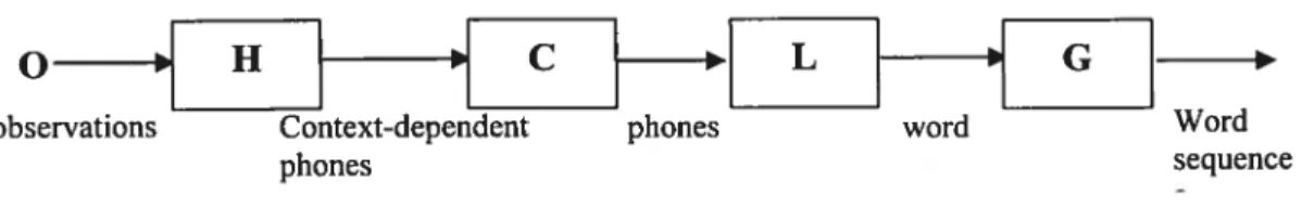
A modem speech recognition system thus consists of two stochastic knowiedge sources, namely the acoustic model and the language model, a lexicon (which in fact may also be a stochastic model), and a phonetic context-dependent network (in case of cross-word modeling) in the search stage [27]. These components are illustrated as a recognition cascade in f igure 2.2.
o____
H _____ C ____ L ____observations Context-dependent phones word Word
phones sequence
figure 2.2 Recognition cascade
In Figure 2.2, H is the union of ail HMMs used in an acoustic modeling which maps sequences of distribution indices to context-dependent phones. C is a phonetic context dependent model which maps context-dependent phones to phones for cross-word modeiing. L is a pronunciation dictionary or lexicon which maps phonemic transcriptions to word. G is a language model, usualiy a 3-gram language model is used.
Once the whole speech recognition network is built, Viterbi decoding [42] is usually used to compute the most likely state sequence for an unknown input ullerance. Trace back through this sequence then yields the most likely phone and word sequences.
Decoding is a very complex search problem for LVCSR, especially when context dependent phone mode! and n-gram language model are used. A standard scheme for reducing search costs uses multiple passes over the data. The output of each pass is a lattice of word sequence hypotheses rather than the single best sequence. This allows the output of one recognition pass to constrain the search in the next pass. An initial pass can use simple models when the search space is large and later passes can use more refined models when the search space is reduced.
However, the weighted transducer approach makes the decoding become easy and fast without resorting to complex schemes. This will be described in detail in the following chapters.
2.2
finite-State Devices
finite-state devices, such as finite-state automata, graphs, and finite-state transducers
have been known since the emergence of Computer Science and are extensively used in areas such as program compilation, hardware modeling, and database management. Although finite-state devices have been known for a long time, more powerful formalisms such as context-free grammars or unification grammars have been preferred in computational linguistics. However, the richness of the theory of finite-state technology and the mathematical and algorithmic advances resulted in the recent study in the field of finite-state technology have had a great impact on the representation of electronic dictionaries, natural language, and speech processing. As a resuit, significant developments have been made in many related research areas [7, 1$, 26, 29, 34].
Some of the most interesting applications of finite-state machines are concerned with computational linguistics [4, 21, 22, 24, 25]. We can describe these applications from two different views. Linguistically, finite automata are convenient since they allow us to describe easily most of the relevant local phenomena encountered in the empirical study of language by compact representations [5]. Parsing context-free grammars can also be deait with using finite-state machines, the underlying mechanisms in most of the methods used in parsing are related to automata [6]. from the computational point of view, the use of finite-state machines is mainly motivated by considerations of time and space
efficiency. Actually, the effect of the size increase on time and space efficiency is the main computational problem flot only in language and speech processing but also in modem computer science. In language and speech processing, time efficiency is achieved by using deterministic (or sequential) automata. In general, the running time of deterministic finite-state machines for specific input depends linearly only on the size of the input. Space efficiency is achieved with classical minimization algorithms for deterministic automata. Applications such as compiler construction have shown deterministic finite automata to be very efficient [161.
In speech recognition the Weighted Finite-State Transducer (WFST) approach has been considerably studied recently [17, 18, 19, 21, 22, 25, 26, 28, 29]. WfSTs provide a powerfiil method for manipulating models of human language in automatic speech recognition systems due to their common and natural representations for HMM models, context-dependency, pronunciation dictionaries, grammars, and alternative recognition outputs. Moreover, these representations can be combined by general transducer operations flexibly and efficiently [17, 2$]. An efficient recognition network including context-dependent and HMM models can be built using weighted determinization of transducers [18, 22]. The two most important transducer operations, weighted determinization and minimization aÏgorithms, can optimize time and space efficiency. The weights along the paths of a weighted transducer can be distributed optimally by applying a pushing algorithm.
Sequential finite-state transducers are very important devices in natural language and speech processing [18, 19, 20]. Sequential finite-state transducers, simply sequential transducers are also called deterministic transducers. This concept is an extension from deterministic automata to transducers with deterministic inputs. That is a machine which outputs a string or/and weights in addition to accepting (deterministic) inputs.
Hereafier a detailed description of the related finite-state devices used for language processing and speech recognition is given. As basic concepts, we first give an introduction on the definitions and properties of finite-state automata and finite-state
transducers. Then we consider the case of string-to-string transducers, which have been successfully used in the representation of large-scale dictionaries, computational morphology, and local grammars and syntax. Considered next are sequential string-to weight transducers or so called deterministic weighted acceptors. These transducers are very useful in speech processing. Language models, phoneme lattices, and word laffices are among the obj ects that can be represented by these transducers.
2.2.1 Finite-State Automata
finite-State Automata (FSA) can be seen as defining a class of graphs and also as defining languages. The following is a simple description on the definitions of f SA and some closure properties. Other information, such as deterministic F$A (sequential F$A), decidability properties, and space and time efficiency discussion are available from references [4, 31, 35, 36].
2.2.1.1 Definitions
FSA:
A finite-state automaton A is a 5-tuple
(, Q,
1 F, E’), where: • is a finite set called the alphabet•
Q
is a finite set of states • IcQ
is the set of initial states • FcQ
is the set of final states• EQx(u {E})xQisthesetofedges.
By this definition f SA can be seen as a class of graphs.
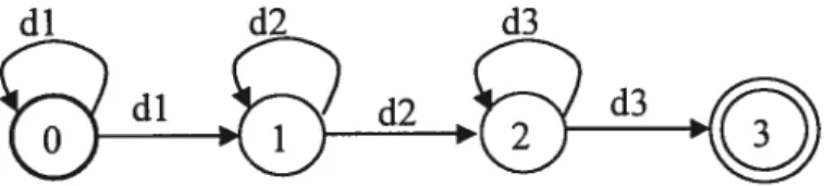
figure 2.3 is a finite-state automaton example. It represents a typical left-to-right, three distribution-HMM structure for one phone, with the labels along a complete path specifying legal sequences of acoustic distributions for that phone.
Figure 2.3 A finite-state automaton example
Extended set of edges:
The set of strings built on an alphabet is also caiied the free monoid . The formai
definition of the star * operation can be found in reference [28J. The extended set of edges E
Q
x xQ
is the smallest set such that(i) Vq e
Q,
(q, 6,q) e E(ii) Vw e and Va e u
{},
if(qi, w, q) e E and (q, a, q3) e E then (qi, w.a, q3) e E, where.stands for concatenation.Extended transition function:
The transition function d of a FSA is a mapping from
Q
x(
u {E}) to 2, and satisfies d(q’, a) = {q e Qj(q’, a, q) e E}. The extended transition function d, mapping fromQ
xonto 2, is that function such that (i) Vq e
Q,
d(q, 6) = {q}(ii) Vw e and Va e u
{},
d(q, w.a)= LJq,Ed(q, w) d(qj, a)Now, a ianguage L(A) can be defined on finite-state automaton A: L(A){w e *,jeJId(j,w)nFØ}
A ianguage is said to be regular or recognizable if it can be defined by an FSA.
2.2.1.2 Closure Properties
The set ofrecognizable ianguage is closed under the following operations:
(1) Union. If A1 and A2 are two FSAs, it is possible to compute an F$A A1 u A2 such that LA1 u A2)=LÇ41) u LtA2).
(2) Concatenation. If A1 and A2 are two f SAs, it is possible to compute an FSA
A,.A2 such that L(A,.A2) = L(A,).L(A7).
(3) Intersection. If A, =
(, Q,,
1,, F,, E,) and A2(, Q.,
£7, F2, E2) are two f SAs, it is possible to compute an f SA denoted A, n A2 such that L(A, n A2) =L(A,) n L(A2). Such an automaton can be constructed as follows:A, n A2=
(, Q]
X Q2, (1,, 12), F, X F2, E) withE=
L]
(qj,a,rj)€Ej, (q2,a,r2)EE2 {((q,,q2),a,(r,,r7))}.(4) Complementation. If A is an FSA, it is possible to compute an f SA —A such that L(-A) =
-L(A).
(5) Kleene Star. If A is an FSA, it is possible to compute an f SA A* such that L(A*)=L(A)*.
2.2.2 Mathematical Foundations for Finite-State Transducers
Before introducing the finite-state transducers we have to give a description about their mathematical foundations. In this section the mathematical foundations such as semiring, power series, weighted transductions, and languages are described in detail.
2.2.2.] Semiring
The semiring abstraction permits the definition of automata representations and algorithms over a broad class of weight sets and algebraic operations [31]. A semiring
(K
, ®, 0, 1) is a ring that may lack negation. It consists of a set K equiped with an
associative and commutative operation
,
called collection, and an associative operation0, called extension, with identities O and 1, respectively, such that 0 distributes over
and 0 0 a = a O 0=0. In other words, a semiring is similar to the more familiar ring
algebraic structure (such as the ring of polynomial over the reals), except that the additive operation may flot have an inverse. for example, (N, +, , 0, 1) is a semiring, where O and 1 are respectively the identity element for+ and operations with + for collection and
The weights used in speech recognition oflen represent probabilities. The appropriate semiring to use is then the probability semiring (R, +, , 0, 1). However, impiementations
ofien replace probabilities with (negative) log probabilities for numerical stability. The appropriate semiring to use is then the image by -log ofthe semiring (R, +, , 0, 1) and is
called the log semiring.
An important example in speech recognition is the min-sum semiring or tropical semiring, (R+ u {co}, mm, +, co, 0) with min for collection and + for extension. Another semiring (* u {cc}, A, •, cc,
)
, called string semiring, is also ofien used in speechrecognition, where , aiso cailed a free monoid, defines a set of strings built on an alphabet , A longest common prefix operation, and • concatenation operation, cc a new
e1ementsuchthatforanystringwE(* u{co})(wAcc=ccAw=wandw.co=co.w
= co). The cross product oftwo semirings defines a new semiring.
Some definitions and caiculations invoive collecting over potentially infinite sets, for instance the set of strings of a language. Cleariy, collecting over an infinite set is aiways well-defined for idempotent semirings such as the min-sum semiring, in which a + a = a
Va e K More generally, a closed semiring is one in which collecting over infinite sets is well-defined.
2.2.2.2 Power $eries
A formai power series S: xi—($,x) is a function from monoid to a semiring (K
e,
®,
Ô,
1). Rationai power series are those formai power series that can be built by rational operations (concatenation, sum, and Kleen closure) from the singleton power series given by ($,x) = k, ($,y) =Ô
if xy for xE, kEK The rationai power series are exactly thoseformal power series that can be represented by weighted acceptors which we wili discuss later in this chapter. A formai power series $ is rationai iff it is realizabie by a weighted acceptor (recognizable) [9].
2.2.2.3 Weighted Transductions and Languages
A weighted transduction T is a mapping T: Ix T— K where E’ and T are the sets of strings over the alphabets and f, and K is an appropriate weight structure; for instance the real numbers between O and 1 in the case ofprobabilities.
A weighted Ïanguage L is a language satisfying the mapping L: 2— K. Each transduction S: x I* K has two associated weighted languages, its flrst and second projections ri(8): E— K and n(S): T—* K, defined by
,r (S) (s) = r S(s, t)
r,(S)(t) = t)
2.2.3 Finite-State Transducers
Finite-state Transducer (FST), also called string-to-string transducer, is an extension from FSA. Each arc in FST is labeled by a pair of symbols rather than by a single symbol. A string-to-string transducer is defined on a string semiring.
2.2.3.1 Definitions FST:
A finite-State transducer is a 6-tuple (E1, E2,
Q,
i, F, E), where:• E1 is the input alphabet among a finite set • E2 is the output alphabet among a finite set
•
Q
is a finite set of states • i eQ
is the initial state • F ciQ
is the set of final states• E
Q
x Ei* x E2* xQ
is the set ofedgesPath:
If an FST T = (E1, E2,
Q,
I, F,E),
a path of T is a sequence ((p1,a1,b,q1)),=i, of edges Esuch that q =pi+j for i = 1 to n-1. Where, (p1,a1,b1,q1) is an edge, q is a state which can be
Successful path:
Given an F$T T=(ri, 2,
Q,
I, F, E), a successful path ((pj,aj,bj,q))1=i, of Tis a path of T such thatpi = iand qn E F.These definitions only are part of important definitions on Finite-state transducers and will be frequently used in the following sections. Other definitions and closure properties (for example Union, Inversion, Letter transducer including E-free transducer and Composition) on FSTs can be found from the literature [12, 26].
2.2.4 Sequential Iransducers
Sequentiai transducers are the most useful transducers used in natural language and speech processing. Many works have been done on this topic [1$, 19, 20, 21, 22].
In language and speech processing, sequential transducers are defined as transducers with a deterministic input (string or just a symbol). At any state of such transducers, at most one outgoing arc is labeled with a given element of the alphabet. This means the input is distinct. The output label might be a string (or a single symbol), inciuding the empty string . 0f course, the output of a sequential transducer is flot necessarily deterministic.
The formai definition of a sequential string-to-string transducer is as foliows: A sequential transducer is a 7-tupie
(Q,
1, F , A, o), where:•
Q
is the set of states • f EQ
is the initial state • F EQ,
the set of final states• and A, finite sets corresponding respectively to the input and output alphabets of the transducer
• c5 the state transition function which maps
Q
x toQ
• u, the output function which maps
Q
x to A*6 and u are partial functions (a state q E
Q
does not necessarily admit outgoing transitions labeled on the input side with ail elements of the alphabet). These functions can be extended to mappings fromQ
x by the following classical recurrence relations:VseQ,Vwe*,Vae,
6(s,E)=s,6(s,wa)=6(6(s,w),a); u(s, ) = u(s, wa) = u(s, w) u(6(s, w), a).Thus, a string w E is accepted by T ifft5(i, w) E f, and in that case the output of the
transducer is u(i, w).
2.2.5 Subsequential and p-Subsequential Transducers
Subsequential transducers are an extension of sequential transducers. By introducing the possibility of generating an additional output string at the final states the application of the transducer to a string can then possibly finish with the concatenation of such an additional output string to the usual output. Such extended sequential transducers with an additional output string at final states are called subsequential transducers.
Language processing ofien requires a more general extension. Indeed, the ambiguities encountered in language (for example ambiguity of grammars, ambiguity of morphological analyzers, or ambiguity of pronunciation dictionaries) can flot be handled by sequential or subsequential transducers because these devices only have a single output to a given input. Since we can not find any reasonable case in language in which the number of ambiguities would be infinite, we can efficiently introduce p-subsequential transducers, namely transducers provided with at mostp final output strings at each final state to deal with linguistic ambiguities. However, the number of ambiguities could be very large in some cases. Notice that 1-subsequential transducers are exactly the subsequential transducers. figure 2.4 shows an example of a 2-subsequential transducer.
A very important concept here is the sequential/p-subsequential function. Similarly, we define sequential/p-subsequential functions to be those functions that can be represented by sequential/p-subsequential transducers. The following theorems give a brief introduction on the characterizations and properties of subsequential and p-subsequential flrnctions (of course, also that of sequential and p-subsequential transducers). Here, the
a.a
expression p-subsequential means two things, the first is that a finite number of ambiguities is admitted, the second indicates that this number equals exactlyp.
Theorem 2.2.5.1 (composition):
Let
f:
* —> \* be a sequential/p-subsequential and g : A’ Q* be a sequential/qsubsequentiai function, then g ofis sequential/pq-subsequentiai. The details about transducer composition are described in Chapter 3. Theorem 2.2.5.2 (union):
Let
f:
Z’ > z\* be a sequential/p-subsequential and g : Ç* be a sequential /qsubsequential function, then g +fis 2-subsequentia1/v + q)-subsequential.
The linear complexity of their use makes sequential and p-subsequential transducers both mathematicaily and computationally of particular interest. However, flot ail transducers, even when they realize functions (rational ffinctions), admit an equivaient sequential or subsequentiai transducer. More generally, sequential functions can be characterized among rationai functions by the following theorem.
Theorem 2.2.5.3 (characterization of seguential function):
Letfbe a rational function mapping to A*. fis sequentiai iff there exists a positive integer K such that:
Vu e , Va e
, w e A,
Iwi
K:f(’ua,) =f(u)wThat is, for any string u and any element a,J(ua) is equal toj(u) concatenated with some bounded string, Notice that this implies thatJ(u) is aiways a prefix ofj(ua), and more generally that iffis sequential then it preserves prefixes.
The fact that flot ail rational functions are sequentiai could reduce the interest of sequential transducers. The following theorem shows however that transducers are exactiy compositions of lefi and right sequential transducers.
Theorem 2.2.5.4 (composition of left and riht seguential transducers):
Letfbe a partial fiinction mapping ‘ to A*. fis rationai iff there exists a lefi sequentiai
Lefi sequentiai fiinctions or transducers are those we previously defined. Their application to a string proceeds from left to right. Right sequential fiinctions apply to strings from right to lefi. According to the theorem, considering a new sufficiently large alphabet Q allows one to define two sequential functions 1 and r decomposing a rationai functionf This resuit considerably increases the importance of sequentiai functions in the theory of finite-state machines as well as in the practical use oftransducers.
Sequential transducers offer other theoretical advantages. In particular, while several important tests such as the equivalence are undecidable with general transducers, sequential transducers have the following decidability property.
Theorem 2.2.5.5 (decidability):
Let T be a transducer mapping to A*. It is decidable whether T is sequential.
The following theorems describe the characterizations of subsequential and p subsequentiai functions.
Theorem 2.2.5.6 (characterization of subseg uential function): Letfbe a partial function mapping to A. f is subsequential iff:
(1) fhas bounded variation
(2) for any rational subset YofA*,f4(Y) is rational
Theorem 2.2.5.7 (characterization of p-subseguential function):
Let
f
=(f,
...,f,,)
be a partial function mapping D o m(/) c to (ts.’)”.f
is psubsequential iff:
(1) fhas bounded variation
(2) for ail i (1 Ip) and any rational subset YofA*,J7’(Y) is rational
Theorem 2.2.5. $ (characterization of p-subseguential function):
Let fbe a rational function mapping to
f
is p-subsequential iff it has bounded variation.2.2.6 Strïng-to-Weight Transducers/Weighted Acceptors
A Weighted finite-state Acceptor (WfSA), or a string-to-weight transducer is a finite state automaton, A, that has both an alphabet symbol and a weight, from some set K, on each transition.
2.2.6.] Definition and Properties of Weighted Finite-state Acceptors
The definition of WFSA is based on the aigebraic structure of a semiring, S=(K , 0, 0,
1).
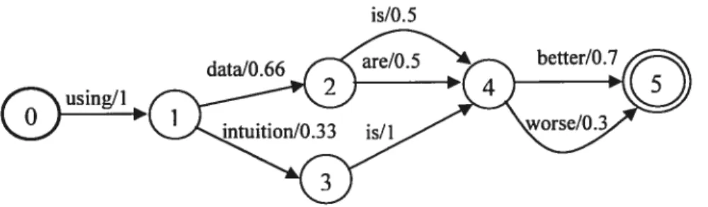
Weighted finite-state acceptors or simpiy weighted acceptors are transducers with input strings and output weights. Figure 2.4 gives an exampie of a weighted finite-state acceptor, which represents a toy language model.
is/O.5
Figure 2.5 A weighted finite-state acceptor
Given a semiring (K, , 0, 0, 1), the formai definition of a weighted acceptor is as
follows:
A weighted acceptor T is defined by T=
(Q,
, L F, E, ). p over the semiring K, where:•
Q
is a finite set of states • the input alphabet• Ic:
Q
is the set of initial states • FQ,
the set of final states• E
Q
x x R÷ xQ
a finite set of transitions, where R, is the output weight• 2 the initial weight function mapping I to R÷ • p the final weight function mapping F to L
Cornpared to the definition of a transducer, we can define for T a partial transition function 5mapping
Q
X to 2 by:V(q, a) e
Q
x 2 cq, u) = {q’Ix
e R+: (q, ci, x, q’) e E},and an output flinction mapping E to R+ by: Vt=(p, u, x, q) e E, a(t)=x.
The following concepts and extensions are very important for string-to-weight transducers. Although we have defined some of them in section 3 in general, more details based on string-to-weight transducers areintroduced.
A path rtin Tfrom q e
Q
to q’ eQ
is a set of successive transitions from q to q’: Yr=((qo,a, X, qi), ..., (q,,,.i, a,j, Xm1,, q,,,)), with V I e [O, m-i], qj+j e 8(q, a’). We can extend
the definition of uto paths by: a(ft) xoxj.
The rt e q q’
I
w refers to the set of paths from q to q’ labeied with the input string w.The definition of 6can be extended to
Q
x by:VRc:Q,Vwe *,R,w)UqER q,w).
The minimum of the outputs of ail paths from q to q’ labeled with w is defined as: 9 (q, w, q )=mina,, (q-q) w a(it).
A successful path in T is a path from an initial state to a final state. A string w e is accepted by T iff there exists a successflul path iabeled with w: w e I, w) n F. The output corresponding to an accepted string w is then obtained by taking the minimum of the outputs of ail successful paths with input label w:
mm(i,J e IxF:Je i, w)(2(i)+ 9(1, w,J + p(J).
A transducer T is said to be trim if ail states of T belong to a successftil path. Weighted acceptors ciearly realize functions mapping to R+. Since the operations we need to consider are addition and mm, and since (R+ {co}, mm, +, co, O) is a semiring, Hence these functions are formai power series. They have the following characterizations which we imported from formai language theory [1, 31]:
1) (5, w) is the image of a string w by a formai power series S. (S, w) is called ffie coefficient of w in S,
2) by the coefficients, S=,, * (S, w)w can be used to define a power series,
supp(S)= {w e : (S, w) co}.
A transducer T is said to be unambiguous if for any given string w there exists at most one successful path labeied with w.
2.2.6.2 Sequential String-to- Weight Transducers/Weighted Acceptors
Recali that a transducer is said to be sequential if its input is deterministic, that is, if at any state there exists at most one outgoing transition iabeled with a given element of the input alphabet . Sequential weighted acceptors have many advantages over non
sequentiai weighted acceptors, such as time and space efficiency. But flot each weighted acceptor has an equivaient sequential weighted acceptor [18, 29]. The formai definition of a sequentiai weighted acceptor/string-to-weight transducer is foiiows:
Definition 2.2.6.1 (seguential weighted acceptor):
A sequentiai weighted acceptor T=
(Q,
i, F, , c5, o, 2, p) is an 8-tuple, where:•
Q
is the set of its states • I eQ
its initial state• Fci
Q
the set of final states • the input alphabet• 6 the transition function mapping
Q
x toQ,
6 can be extended as in the string case to mapQ
x toQ
• u the output function which maps
Q
x to R+, c can aiso be extended toQ
x• 2 e R+ the initial weight
• p the final weight function mapping F to L
A string w e is accepted by a sequential acceptor T if there existsf e F such that i, w)
=f
Then the output associated to w is: 2+ a(i, w) +pQ).Considering the benefits of time and space efficiency, the sequentiai transducer or acceptor is preferred in language and speech processing. But, like we mentioned before, not ail transducers are sequential transducers. The process used to transfer a non sequential transducer to an equivaient sequential transducer is called determinization. Unfortunately, flot ail transducers have an equivaient sequentiai transducer, which also
means that not ail transducers can be determinized. The following definition can be used to determine whether a transducer can admit determinization.
Definition 2.2.6.2 (determinization):
Two states q and q’ of a string-to-weight transducer T
(Q,
I f, , 5 u, 2, p), flotnecessarily sequential, are said to be twins if:
V(u, y) e (*)2, ({q, q’} J u), q e q, y), q’ e q’, y)) = q, y, q)= q’, y, qr).
If any two states q and q’ of a string-to-weight transducer T are twins we say T has twins property. If a string-to-weight transducer has twins property it is determinizable. Notice that according to the definition, two states that do flot have cycles with the same string y are twins. In particular, two states that do flot belong to any cycle are necessarily twins. Thus, an acyclic transducer has the twins property.
The following theorem gives an intrinsic characterization of sequential power series: Theorem 2.2.6.1 (characterization of seguential power series):
Let S be a rational power series defined on the tropical semiring. $ is sequential iff it has bounded variation.
The proof on this theorem is based on twins property [3].
2.2.7 Weighted Transducers
Weighted finite-state Transducers (WFSTs), or simply weighted transducers, are also called string-to-string/weight transducers (S$WTs). The definition of string-to string/weight transducers is similar to the definition of string-to-string transducers or string-to-weight transducers. The only difference is that the output of a string-to stringlweight transducer is a pair composed by a string and a weight. The SSWTs generalize WF$As by replacing the single transition label by a pair (I, o)of an input label I and an output label o. While a weighted transducer associates symbol sequences and weights, a WF$T associates pairs of symbol sequences and weights, that is, it represents a weighted binary relation between symbol sequences [11, 44].
2.2. 7.1 GeneraÏ Weighted Transducers
A weighted transducer T is defined by T=
(Q,
, A, ï, f, E, X, p),where:
•
Q
is a finite set of states• 1 and A, finite sets corresponding respectively to the input and output alphabets ofthe transducer
• 1 E
Q
is the initial state • F ciQ,
the set of final states• Ec:QxxAxR±xQafinitesetoftransitions
• 2 the initial weight function mapping I to L • p the final weight function mapping f to L
The set E can be extended to include transitions
Q
x x A x R+ xQ,
where their input and output can be strings.Without extension of E, it defines the weighted transducers used in our CSR research. Each arc of these transducers has a feature that its input and output are symbols like in Figure 2.5. The symbol refers to a string with a length equals to 1 or O (an empty string E).
2.2.7.2 $equential Weighted Transducers
The sequential transducers described here are transducers with a deterministic input. At any state of such transducers, at most one outgoing arc is labeled with a given element of the alphabet.
A sequential weighted transducer T=
(Q,
1, F, , A, 6, a, X, p), where:•
Q
is the set of its states• ï ê
Q
its initial state• f
Q
the set of final states• and A, finite sets corresponding respectively to the input and output alphabets ofthe transducer
• Sthe transition function mapping
Q
x toQ
• uthe output function which mapsQ
x to A x R+ • 2 ê L the initial weight• p the final weight function mapping f to R+
The transition function 6 can be extended as in the string case to map
Q
x toQ,
and the output function ucan also be extended toQ
x to A* x L.If the extensions of 6 and u are not allowed, the defined sequential weighted transducers wiil have only symbois as input and output of their arcs like in figure 2.5. This type of sequential weighted transducers are widely used in current CSR researches.
Even though the sequential property is expected, not ail weighted transducers are sequential. In fact, in most cases the original transducer is flot sequentiai. Therefore a determinization algorithm is needed.
In this chapter we have reviewed the principÏes and architecture of modem CSR systems and then described the formai definitions and properties of finite-state devices inciuding automata, string-to-string transducers, weighted acceptors, and weighted transducers. In the next chapter we will describe some weighted acceptor and transducer operations.
Chapter 3
Weighted Acceptor and Transducer Operations
Like unweighted acceptors, weighted acceptors and transducers also have a common set of finite-state operations to combine, optimize, search, and prune them [26]. Each operation implements a single, welY-defined function that has its foundations in the mathematical theory of rational power series [il,
441.
Many of those operations are the extensions of classicai algorithms for unweighted acceptors to weighted transducers.3.1 Basic Operations
The basic operations, like union, concatenation, KÏeene closure, etc., combine transducers in parallel, in series, and with arbitrary repetition, respectively. Other operations include projection, best path, N-best path, pruning, topoÏogicaÏ sort reversal E-removal inversion, etc. Projection converts transducers to acceptors by projecting onto the input or output label set (Jrojection). Best path or N-best path finds the best or the N best paths in a weighted transducer. Pruning removes unreachable states and transitions. Topological sort operation sorts acyclic automata topologically, that is to number states by satisfying the condition j
j
for any transition from a state numbered i to a state numberedj.
Reversal consists of reversing ail transitions of the given transducer, transforming final states into initial states and initial states into final states. E-removal operation removes ail transitions for which the input or output symbois are E. Inversion operation inverses the transducer by swapping the input with output symbols on transitions.In foliowing sections a few important operations that support the speech recognition applications are described in detail.
3.2 Composition
The composition operation is the key operation on transducers and is very useful since they ailow the construction of more complex transducers from simpler ones.
3.2.1 Theoretical Definition and Operation
Given two transductions Tj: fx T— K and T2: 1x T— K, we can define their composition T1 O
T2 by
(Tj °
T,)(r,t) = I(r,s)®T2(s,t)
Leaving aside transitions with E inputs or outputs for the moment, the following mie specifies how to compute a transition of T1 O
T2 from appropriate transitions of T1 and T2 (qi a.b/w >qi ‘and q b.c/w, > q.?’) => (qi, q) a.c/(w10w2) > (q q’)
where s x;1’#‘
> represents a transition froms to twith input x, output y and weight w. For example, ifS represents F(siIs) and R P(,Is, $°
R represents P(sIs). It is easy to see that composition °
is associative, that is, in anytransduction cascade Si O
52 °S,,, the order of association of °
operations does flot matter.
The composition of two transducers represents their relationai composition. In particuiar, the composition T = R ° S of two transducers R and S has exactly one path mapping
sequence u to sequence w for each pair of paths, the first in R mapping u to some sequence y and the second in S mapping y to w. The weight of a path in T is the 0-product of the weights of the corresponding paths in R and S [11, 44].
Composition is useful for combining different levels of representations. For instance, it can be used to apply a pronunciation lexicon to a word-levei grammar to produce a phone-to-word transducer whose word sequences are restricted to the grammar. Many kinds of CSR network combinations, both context-independent and context-dependent, are conveniently and efficientiy represented as compositions.
The composition aigorithm generalizes the ciassical state-pair construction for finite automata intersection [18] to weighted acceptors and transducers [7, 29]. The composition R OS of transducers R and S has pairs of an R state and an S state as states, and satisfies the following conditions:
(1) its initial state is the pair ofthe initial states of R and S;
(2) its final states are pairs of a final state of R and a final state of S, and
(3) there is a transition t from (r, s) to (r’, s’) for each pair of transitions tR from r to r’
and tg from s to s’ such that the output label oft matches the input label of t’. The
transition t takes its input label from tR, its output label from t, and its weight is the
Ø-product of the weights oftR and t5when the weights correspond to probabilities.
Since this computation is local, i.e. it involves only the transitions leaving two states being paired and can thus be given a lazy implementation in which the composition is generated only as needed by other operations on the composed machine. Transitions with
labels in R or $ must be treated specially as we will discuss later.
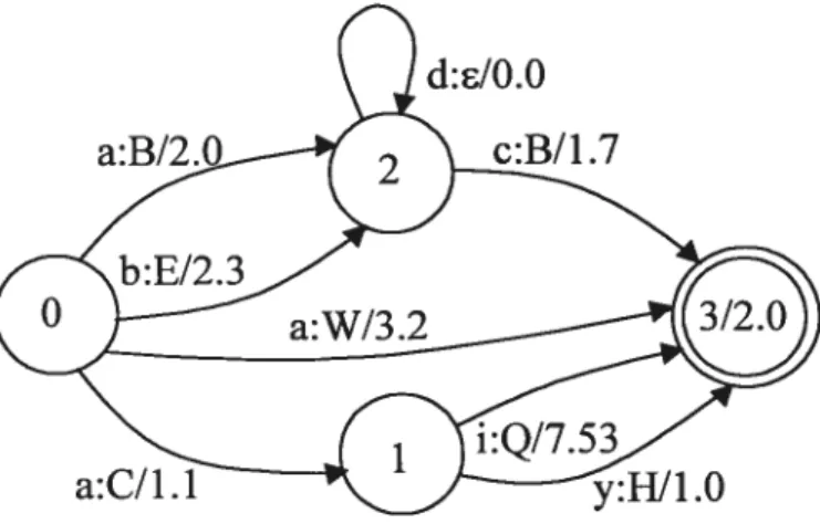
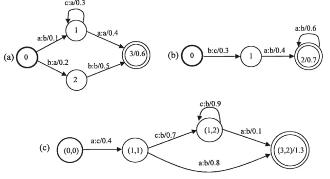
Figure 3.1 shows two simple E-free transducers over the tropical semiring, Figure 3.1 a and Figure 3.1 b, and the resuit of their composition, figure 3.1 c. The weight of a path in the resulting transducer is the sum of the weights of the matching paths in R and $ since in this semiring, ® is defined as the usual addition (of log probabilities).
c:aJO.3 a:b/O. 1 a:aIO.4 (a) (b) (c) a:b/O.6
Since weighted acceptors are represented by weighted transducers in which the input and output labels of each transition
are
identical, the intersection oftwo
weighted acceptors is just the composition ofthe corresponding transducers.3.2.2 Composition Algorithm
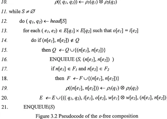
3.2.2.1 -free composition
Given two -free transducers T1 =
(Qj,
, A, Ii F1, E1, %j, pj)and
T2 = (Q2, , A, ‘2, F2,E2, )2, p2), the resuit of the composition of T1 and T2 is transducer T=
(Q,
, A, j, F, E, 2,p). In this algorithm, transitions are combined using the ®-product associated with the semiring over which the transducer is defined. To show the algorithm some notations
are
introduced:1. For qE
Q,
E[q] represents the set of transitions leaving q, 2. ForeEE,t) i[e]represents the input label ofe,
ii) o[e] represents the output label ofe,
iii)w[e]represents the weight ofe,
iv) n[e] represents the destination state ofe.
Now the E-free composition
can
be shown as the following pseudocode:COMPOSITION (T1, T2): 1. 8—Q—E—I—F—Ø 2. foreachqjEl1 3. doforeachq2EL 4. do
Q
‘—Qu{(qj,q2)} 5. 16—ILJ{(qj,q2)}6.
%((
qi, q)) — %i(qi) ® %2(qI)7. ENQUEUE (S, (qi, q))
8. ifqjEFiandq2EF2
10. q,, q)) +—pi(qj)®p2(q2)
11. while$ø
12. do(qj,q2)—head[Sj
13. for each
(
e, e2) E E[qi] x E[q2J suchthat o[ejJ = i[e2] 14. do if(n[ejJ, n[e2])Q
15. thenQ 6—Qu{(n[ej],n[e2J)}
16. ENQUEUE (S, (n[ei], n{e2])
)
17. if n[ejJ E fi and n[e2] e f71$. then f —Fu{(n[ey], n[e2])}
19. ,(n[ej], n{e7])) +—pi(qi) 0p2(q2)
20. E ‘—E u{(( q,, q), i[ei], o[e2], w[ei] O W[e2], (n[eiJ, n{e2])}
21. ENQUEUE(5)
figure 3.2 Pseudocode ofthe E-free composition
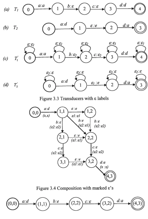
3.2.2.2 General Case Composition
Transitions with labels in T1 or T2 add some subtieties to composition. In general, output and input ‘s can be aligned in several different ways: an output Ein T1 can be
consumed either by staying in the same state in T2 or by pairing it with an input &in T2;
an input in T2 can be handled similarly. for instance, the two transducers in Figure 3.3(a) and (b) can generate all the alternative paths in Figure 3.4. However, the single bold path is sufficient to represent the composition resuit, shown separately in Figure 3.5. The problem with redundant paths is flot only that they increase unnecessarily the size of the resuit, but also they fail to preserve path multiplicity: each pair of compatible paths in
T1 and T2 may yield several paths in T1 ‘
T2. If the weight semiring is flot idempotent, that leads to a result that does not satisfy the algebraic definition of composition.
This path-multiplicity problem can be solved by mapping the given composition into a new composition
T10T2— 1 °F° T
in which f is a special filter transducer and the 1” are versions of the T1 in which the relevant &labels are replaced by special “suent transition” symbols as shown in figure
3.3(c) and (d). The bold path in Figure 3.4 is the only one allowed by the ifiter in Figure 3.6 for the input transducers in Figure 3.3.
(a) T1 b:E .•
(b) T2
(e) i;’
(cT
Figure 3.4 Composition with marked ‘s
Figure 3.5 Composition output Figure 3.3 Transducers with labels
(2:
d:a
(x:x)
By inserting a filter between T1 and T2 (more precisely, between T’ and T) and applying the s-free composition algorithm on this new composition, the redundant paths are removed. Interestingiy, the filter itself can be represented as a finite-state transducer. Fiiters of different forms are possible, but the one shown in Figure 3.6 leads in many cases to the fewest transitions in the resuit, and ofien to better time efficiency [25]. (The symbol x represents any element ofthe alphabet ofthe two transducers.)
The filter can be understood in the following way: as long as the output of T1 matches the input of T2, one can move forward on both and stay at state O. If there is an s-transition in T1 , one can move forward in T1 (only) and then repeat this operation (state 1) until a
possible match occurs which would lead to the state O again. Similarly, if there is an s-transition in T2, one can move forward in T2 (only) and then repeat this operation (state 2) until a possible match occurs which would lead to the state O.
Clearly, ail the operations involved in the filtered composition are also local, therefore they can 5e performed on demand, without the need to perform explicitly the replacement ofT1by 1.
We can thus use the lazy composition algorithm as a subroutine in a standard Viterbi decoder to combine on-the-fly a language mode!, a multi-pronunciation lexicon with corpus-derived pronunciation probabilities, and a context-dependency transducer. The extemal interface to composed transducers does flot distinguish between iazy and precomputed compositions, so the decoder algorithrn is the same as for an explicit network.
3.2.2.3 Complexity
In the worst case, the composed transducer resuits in the combination of ail state-pairs (qi, q) as its states and has at most
EjllE2I
transitions. Thus it takesO(1Q111Q21)
for the creation of states andO(IE1
.IEI)
for the creation of ail transitions. Therefore, the overailcomplexity is:
O(1Q111Q2I +
IE1LIE2I)
3.3
Determinization
A deterministic automaton is non-redundant and contains at most one path matching any input sequence, thus reducing time and space required to process an input sequence. In the same way, a deterministic/sequentiai WFSA needs to eliminate redundancy. Thus it must caiculate the combined weight of ail the paths for a given input sequence. for instance, in the case, common in speech recognition, where weights are interpreted as (negative) logarithms of probabilities, the weight of a path is obtained by adding the weights of its transitions, and the combined weight for an input string is the minimum of the weights of ail paths accepting that string. In the case where weights are probabilities where the overail probability mass of ail paths accepting an input is sought, weights are multiplied along a path and summed across paths. Both cases can be handied by the same algorithm, parameterized with appropriate definitions of the two weight combination operations.
As aforementioned, not ail transducers have an equivalent sequential transducer, which means that not ail transducers can be determinized. The following definition can be used to determine whether a transducer can admit determinization.
Two states q and q’ of a string-to-weight transducer T
(Q,
I, f, , cS u, 2, p), flot necessarily sequentiai, are said to be twins if:V(u, y) e (*)2, ({q, q’} cz u), q e cq, y), q’ e y)) z q, y, q) = q’, V,
q.
If any two states q and q’ of a string-to-weight transducer T are twins, we say T has twins properly. If a string-to-weight transducer has twins property it is determinizable.