Approximate search with quantized sparse representations
Texte intégral
Figure
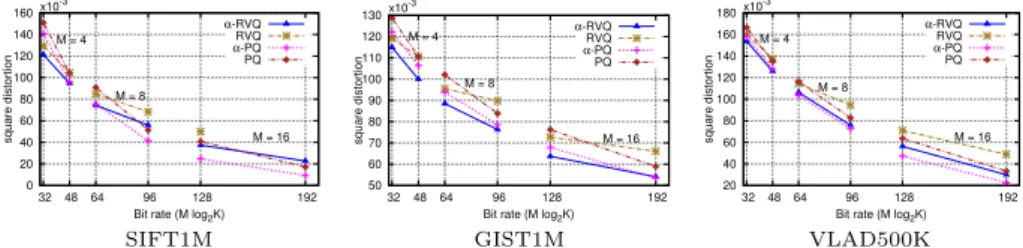
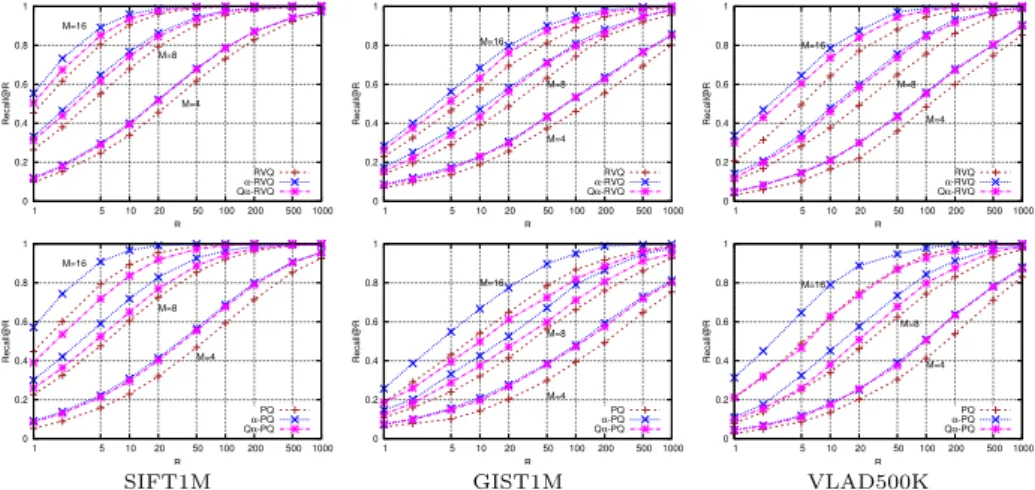
![Fig. 4: Performance comparison for Euclidean-aNN. Recall@R curves on SIFT1M and GIST1M, comparing proposed methods to PQ, RVQ and to some of their extensions, CKM [3], ERVQ [4], AQ [21] and CQ [8].](https://thumb-eu.123doks.com/thumbv2/123doknet/12570515.345817/13.620.57.571.50.165/performance-comparison-euclidean-recall-comparing-proposed-methods-extensions.webp)
Documents relatifs
specially tailored to the Kyrgyz context and it is thus intended to guide the staff of the SE and implementing partners with the objective of supporting them apply Conflict
When reactions were carried out using RuvB L268S , we found that the mutant protein stimulated RuvC-mediated Holliday junction resolution (lanes f and g). The sites of
Swiss Toxicological Information Centre, Zu¨rich, Switzerland and 5 Department of Anaesthesiology, Perioperative and General Intensive Care Medicine, Salzburg General Hospital
Compared to papers reviewed in section 2, the KVQ allows handling linear transformations (compared to metric-based approaches), it is generic (it can be systematically applied to any
La propriété de rigidité diélectrique et la stabilité thermique du Parylene HT (forme commerciale du parylène AF4) sont plus particulièrement détaillées ici,
We provide explicit bounds on the max- imum allowable transmission intervals (MATI) for each segment and we guarantee an input-to-state stability property for the estimation
The latter time point was chosen to analyze the inositol phosphate levels at day-10 differentiating stage, the time point corresponding to neuronal differentiation stage shortly
Foreign advisers and government officiaIs are valuable cata- lysts in the process of educational change, but the vital ingredient is the support of the people of the
