Harmonic Adaptive Latent Component Analysis of Audio and Application to Music Transcription

HAL Id: hal-00945197

https://hal.inria.fr/hal-00945197

Submitted on 24 Mar 2014

HAL is a multi-disciplinary open access

archive for the deposit and dissemination of

sci-entific research documents, whether they are

pub-lished or not. The documents may come from

teaching and research institutions in France or

abroad, or from public or private research centers.

L’archive ouverte pluridisciplinaire HAL, est

destinée au dépôt et à la diffusion de documents

scientifiques de niveau recherche, publiés ou non,

émanant des établissements d’enseignement et de

recherche français ou étrangers, des laboratoires

publics ou privés.

Audio and Application to Music Transcription

Benoît Fuentes, Roland Badeau, Gael Richard

To cite this version:

Benoît Fuentes, Roland Badeau, Gael Richard. Harmonic Adaptive Latent Component Analysis of

Audio and Application to Music Transcription. IEEE_J_ASLP, IEEE, 2013, 21 (9), pp.1854–1866.

�hal-00945197�

Harmonic Adaptive Latent Component Analysis of

Audio and Application to Music Transcription

Benoit Fuentes*, Graduate Student Member, IEEE, Roland Badeau, Senior Member, IEEE and Gaël

Richard, Senior Member, IEEE

Abstract_{—Recently, new methods for smart}

decom-position of time-frequency representations of audio have been proposed in order to address the problem of automatic music transcription. However those tech-niques are not necessarily suitable for notes having variations of both pitch and spectral envelope over time. The HALCA (Harmonic Adaptive Latent Component Analysis) model presented in this article allows consid-ering those two kinds of variations simultaneously. Each note in a constant-Q transform is locally modeled as a weighted sum of fixed narrowband harmonic spectra, spectrally convolved with some impulse that defines the pitch. All parameters are estimated by means of the expectation-maximization (EM) algorithm, in the framework of Probabilistic Latent Component Analysis. Interesting priors over the parameters are also intro-duced in order to help the EM algorithm converging towards a meaningful solution. We applied this model for automatic music transcription: the onset time, dura-tion and pitch of each note in an audio file are inferred from the estimated parameters. The system has been evaluated on two different databases and obtains very promising results.

Index Terms—Automatic transcription, multipitch estimation, probabilistic latent component analysis, nonnegative matrix factorization.

EDICS Category: AUD-ANSY

I. INTRODUCTION

Music transcription consists in describing some physical characteristics of a musical signal by means of some notation system. In many music genres, including western music, a big deal of information is carried on the set of notes played by the instruments, or sources. Classically, a musical note is defined by three attributes: its pitch, duration, and onset time. Automatic music transcription consists in estimating these notes and their attributes given an audio recording (it could also include a clustering of the notes played by a same instrument, but this paper does not address this problem). To this aim, an audio signal is often decomposed into small segments (or frames) on which the pitch of all active notes is estimated. This subtask, called multipitch estimation, is still an open problem, far

B. Fuentes, R. Badeau and G. Richard are with the Département Traitement du Signal et des Images, Institut Mines-Télécom, Télécom ParisTech, CNRS LTCI, 37-39, rue Dareau 75014 Paris, France (e-mail: firstname.lastname@telecom-paristech.fr)

The research leading to this paper was partly supported by the Quaero Programme, funded by OSEO, French State agency for innovation.

from being completely solved. For an overview of the proposed methods for this task, the reader is referred to [1]. Recently, a new class of methods has emerged in order to address automatic transcription problems, which consists in modeling a time-frequency representation (TFR) of audio as a sum of basic elements, atoms, or kernels. For instance, an atom can represent the spectrum of a single note, in which case it will be active whenever the corresponding note is played [2]. Such decompositions, called herein TFR factorizations, are widely used in other fields as well, such as source separation [3], main melody estimation or extraction [4], [5] or beat location estimation [6].

TFR factorization techniques can be roughly grouped into three subclasses whether they are unsupervised, su-pervised or semi-susu-pervised.

Unsupervised factorizations do not use any learning

stages but take advantages of redundancies in musical TFR to estimate both the basic atoms and their activations. This is the case of the classic Non-Negative Matrix Factorization (NMF) [7], [2] where each column of a TFR is modeled as a weighted sum of basic spectra (the kernels). The kernels and the time-dependent weights (the activations) are jointly estimated using an iterative algorithm which minimizes some divergence between the input TFR and the factorization model. Many variants and extensions that better take musical signals characteristics into account have been proposed. See for example the shift-invariant model of [8] or the dynamic model with time-frequency activations of [9]. Those techniques are quite appealing since they only rely on the assumption that music is redundant (e.g. no learning stage is needed). It is then theoretically possible to model any kind of musical event, provided it is repeated over time. However, a major drawback with such techniques is that they are under-constrained, and nothing ensures that the decomposition will be sufficiently informative to perform automatic transcription.

An appealing solution to constrain the decomposition is to perform a supervised factorization. It consists in using fixed kernels, learned during a training stage, or set manually. For example in [10] or [11], several note kernels are first extracted from monophonic recordings of specific instruments. Then, each column of an input TFR is decomposed using those templates as a dictionary. In [11], the kernels can also be shifted in frequencies so this method is robust to detuning or fundamental frequency modulations. If those methods can be very fast ([10] is a real-time online algorithm), and less sensitive to local

minima than unsupervised TFR factorizations, a main drawback is that their performances strongly depend on the similarity between the fixed kernels and the corresponding spectra of the different sources in the input TFR. Solutions to this problem can be proposed though. For instant, in the model put forward in [5], the spectrum resulting from a linear combination of fixed kernels can be shaped by a smooth filter, so that it better fits the observations.

The approaches of the third subclass are based on a

semi-supervised factorization. The principle here is to estimate

both kernels and activations, and to constrain the kernel to lie in some predefined subspace. This subspace can be defined during a learning stage, as in [12] where the notion of hierarchical eigeninstruments is introduced. They represent subspaces, each one of them being used to model a specific class of instruments. Those subspaces are pre-learned and during the factorization stage, one or more eigeninstrument is used to model the note spectra of a source present in the input TFR. The subspace of the kernels can also be set manually. For example, the basic spectra can be modeled as a linear combinations of fixed narrow-band harmonic spectra in order to consider both harmonicity and spectral smoothness of a note spectrum [13]. More simply, the energy of a kernel representing a note can be forced to zero for frequencies between the partials of this note (see [14]). Those methods have many advantages since they ensure both a meaningful factorization and an adaptability to the data.

It is interesting to note that in [12], [13], the hypothesis that the input TFR has redundancies is made. More specifically, it is supposed that a given source in the mixture has note-wise timbre similarities throughout the signal. This supposition reduces the dimension of the pre-defined subspace of the kernels during the factorization step. It is a good assumption for many musical instruments, but not all of them, the human voice being the best counter-example: the timbre depends on the lyrics and not on the sung note. On the opposite, in the model we present in this paper, called Harmonic Adaptive Latent Component Analysis (HALCA), the decomposition is independently performed from one frame to another: no assumption of redundancy is made, and the kernels can stay within all the pre-defined subspace along time. Consequently, it allows considering all kinds of harmonic instruments, having variations of both pitch and spectral envelope over time.

Regardless of the TFR factorization subclass considered, it is also possible to constrain the decomposition by means of the addition of priors or penalty functions. They are ap-plied to the parameters constituting a musical TFR model. Their use can be quite interesting since they act like an inducement for the parameters to converge toward a more likely solution, instead of just constraining the parameters to lie in some subspace. Thus, it is a soft way to add information about the nature of the data to be analyzed. Many priors or penalty terms have been proposed in the literature, such as sparsity or temporal smoothness of the activations [10], [15], [3], [16]. In this paper, three different priors and their derivation are presented: a monomodal

prior for monophonic sources (already introduced in [17]), a sparse prior (partially introduced in [18] in a different framework) and a timbre temporal continuity prior.

Before getting to the main contributions and the overview of this paper, it is important to clarify that there are many mathematical frameworks to perform TFR factorization: analytical models [7], [2], [19], [20], probabilistic NMF [21], [22], Probabilistic Latent Component Analysis (PLCA) and its shift invariant version [23], [15], [8], Gaussian Processes [24], Generalized Coupled Tensor Factorization [25], or non-parametric Bayes [26]. In this paper, the framework used is the PLCA, which offers a convenient way to derive convolutive models and introduce priors. In the HALCA model, an input signal is considered as a mixture of several harmonic sources (monophonic or polyphonic) and a noise component. The notes played by the sources can present temporal variations of both spectral envelope and fundamental frequency over time. The system in [5], which models an input spectrogram as the sum of a component of interest and a residual, presents also similar features. Indeed, the component of interest is a source/filter model which can also consider those two kind of variations. In the model of this component, the sources are a set of fixed harmonic kernels, and the filter is a smooth spectral envelope applied to a linear combination of those sources. However, it is more suitable for a single main instrument (especially monophonic) since only one filter is applied to a sum of fixed kernels. Besides, nothing prevents the model of the residual from modeling musical notes as well. Therefore, this system is more adapted to model an input signal as a mixture of a main instrument and an accompaniment. On the opposite, in the HALCA model, each polyphonic source can have its own time varying spectral envelope, and the noise component is designed so that it cannot consider harmonic notes. The main contributions of this paper include the following:

∙ A generalization of the model presented in [17] for

polyphonic signals.

∙ Besides the two priors of monomodality and sparseness,

already introduced respectively in [17] and [18], the introduction of a new prior over the parameters of a PLCA-based model, that enforces temporal continuity.

∙ For the first time, the HALCA model, as well as

the influence of the priors, are evaluated in a task of automatic transcription.

The paper is organized as follows. First, the Constant-Q Transform (CQT), which is the TFR used in this paper, and the PLCA are introduced in section II. Then, the model we put forward, is explained in section III. In section IV, the three priors are presented. Finally, the application to automatic transcription and the evaluation are described in section V, before concluding in section VI.

II. TOOLS AND FRAMEWORK

A. Constant-Q transform

The system put forward in this paper performs the analysis in the time-frequency domain. Thus, a constant-Q

transform (CQT) [27] is first applied to the audio signal to be analyzed. The CQT is a complex time-frequency representation of a temporal signal, with a logarithmic frequency scale. This characteristic offers a major advantage for musical signals: the spacing between two given partials of a harmonic note remains the same, regardless of its pitch. A change of fundamental frequency can thus be seen as a frequency shift of the partials, and it is possible to devise shift-invariant models, such as the HALCA model presented in this paper. This model takes as input non-negative data, therefore, we apply a positive transformation to the CQT of a signal. Actually, every TFR in this paper are calculated the same way. First, the complex CQT �� �(� and � being

frequency and time indexes) of a monophonic signal, with 3 bins/semitones and a time step of 10ms, is calculated for � from 27.5Hz to 7040Hz (we used the implementation provided in [28]). Then the input data �� � is computed as

follows: �� �=︀♣�� �♣. Using the square root is equivalent

to applying a slight compression on the coefficients, and experiments have shown that the analysis model we present here gives better results that way. By abuse of language, the term CQT will refer to this kind of TFR from now on.

B. Introduction to Probabilistic Latent Component Analysis

PLCA [23] is a tool for non-negative data analysis (in this paper, the data are the non-negative coefficients that compose the magnitude �� �of the CQT of a signal). The

observations �� � are modeled as the histogram of the

sampling of � independent and identically distributed random variables (��, ��) (� from 1 to � is the number

of the draw) that correspond to time-frequency bins. They are distributed according to the probability distribution

� (�, �; Λ), Λ being a set of parameters. The way � (�, �; Λ)

is structured induces the desired decomposition of �� �:

Λ is estimated by maximizing the log-likelihood of the observations given the parameters, or, if there is a prior distribution � �(Λ) of the parameters, the posterior log-probability. One can calculate the log-likelihood function (we denote ¯� the set of variables ¶��♢�=1...�):

�Λ( ¯� , ¯�) = ln︀� ( ¯� , ¯�; Λ) ︃ = ln ︀ ︁ ︁ � � (��, ��; Λ) ︀ ︀ =︁ � ln (� (��, ��; Λ)) =︁ � ︁ �,� 1(�j,�j)(�, �) ln (� (�, �; Λ))

where 1�(�) is the indicator function. That leads to:

�Λ( ¯� , ¯�) =

︁

�,�

�� �ln (� (�, �; Λ)) , (1)

since �� � is considered as a histogram. The posterior

log-probability is then given by (up to an additive constant with respect to Λ):

ln︀� (Λ♣ ¯� , ¯�)︃ = �Λ( ¯� , ¯�) + ln (� �(Λ)) . (2)

In the basic PLCA model, a latent variable � is introduced,

� and � are conditionally independent given �, and � (�, �; Λ)

is modeled as: � (�, �; Λ) =︁ � � (�)� (� ♣�)� (�♣�) =︁ � � (�, �)� (� ♣�),

where Λ is the set of parameters ¶� (�, �), � (�♣�)♢�,�,�.

� (� ♣�) then corresponds to several basic spectra and � (�, �)

to their time activations, similarly to the classic NMF. In the shift-invariant version of PLCA [8], as well as in the HALCA model, � results from the sum of two latent random variables, and � (�, �; Λ) is consequently the convolution of two probability distributions, as we will see in next section. Since there is usually no closed-form solution for the maximization of the log-likelihood or the posterior, the Expectation-Maximization (EM) algorithm is used to estimate the model parameters. In this document, Z and R will refer to the sets of integers and real numbers, ]�, �[ to the set ¶� ∈ R ♣ � < � < �♢ and J�, �K to the set ¶� ∈ Z ♣ � ⊘ � ⊘ �♢.

III. HALCA MODEL

A. Model representation

Let us introduce a first latent variable � in order to decompose the CQT of a musical signal as the sum of a polyphonic harmonic signal (in this case, � = ℎ) and a noise signal (� = �) (the notations �ℎ(.) and ��(.) are

used for � (.♣� = ℎ) and � (.♣� = �)):

� (�, �) = � (� = ℎ)�ℎ(�, �) + � (� = �)��(�, �), (3)

where �ℎ(�, �)(�,�)∈Z×J1,� K and ��(�, �)(�,�)∈Z×J1,� K

respec-tively represent the CQTs of the polyphonic and the noise signal. � (�)�=ℎ,� corresponds to the normalized global

energy of each part. We can now consider the polyphonic part as the sum of � sources (designated by the latent variable �), each of them supposed to represent a single instrument:

�ℎ(�, �) =

︁

�

�ℎ(�, �, �). (4)

Each column of �ℎ(�, �, �) then represents the spectrum of

one or more harmonic notes, played by a single instrument (we suppose that all instruments are harmonic). Let us see now how each column of �ℎ(�, �, �) and ��(�, �) is modeled.

1) Instrument model: In order to account for the

non-stationary nature of many musical instruments in terms of both pitch and spectral envelope, the model used for one in-strument is the same as in [17]. This model allows consider-ing simultaneously those two kinds of non-stationarities. At time �, the spectrum of source �, represented by �ℎ(�, �, �),

is decomposed as a weighted sum of � fixed narrow-band harmonic spectral kernels, or kernel distributions, denoted

�ℎ(Û♣�)(Û,�)∈J1,� K×J1,�K, spectrally convolved by a

time-frequency impulse distribution �ℎ(�, �, �)(�,�)∈J1,�K×J1,� K (�

is then defined as the sum of the two random variables Û and �):

�ℎ(�, �, �) =

︁

�,�

The parameters have the following characteristics:

∙ all kernels �_ℎ(Û♣�) share the same fundamental

fre-quency, but have their energy concentrated at a given harmonic (their design will be discussed later in section III-A4),

∙ the weights applied to the kernel distributions, denoted

�ℎ(�♣�, �) and called envelope coefficients, define the

spectral envelope of the notes played at time � by source �,

∙ each column of the impulse distribution �_ℎ(�, �, �)_�can

be unimodal or multimodal, each mode corresponding to the pitch of one note,

∙ in order to ensure that the model can fit any spectral

spreading of the partials (for instance, a continuous variation of pitch induces a larger spreading at a given time), kernels have energy only for the frequency bins corresponding at harmonics and the spreading is taken into account in the impulse distribution.

Fig. 1 illustrates this instrument model. In this model,

Time Frequency f (frequency) An instrument spectrum i (frequency)

+

*

Fixed harmonic kernels

µ (frequency)

µ (frequency)

µ (frequency)

Fig. 1. Spectrum model for source � at time �. Each kernel has its main energy concentrated on a given harmonic (multiple of a reference fundamental frequency), and the rest of the energy is shared between

adjacent partials _.

the spectral shape of each note can evolve over time. However, we need to suppose that at given � and �, all simultaneous notes of a single source have the same spectral shape. This hypothesis is not very realistic for real music instruments, but it does not appear to be critical for the application to music transcription, as we will observe in section V. The following remark can help to understand why. In practice, one source does not necessarily represent a specific instrument: several sources can be used to model a single real instrument, and one source can contribute to the modeling of several notes played by several instruments. Thus, we could say that a source represents a “meta-instrument”. For automatic transcription, as we mean it (i.e. with no clustering of the notes with respect to the instruments), this characteristic is not a problem since only the global impulse distribution, defined as

�ℎ(�, �) =︀��ℎ(�, �, �) will be used to estimate the onset,

offset and pitch of each note.

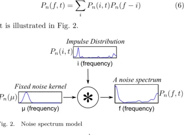
2) Noise model: In order to consider smooth structures

in a CQT, the noise is modeled as the convolution of a fixed smooth narrowband window, ��(Û) and a noise impulse

distribution ��(�, �) (the term impulse is no longer relevant

in this case, but we keep it for the sake of consistency). The model can be written:

��(�, �) = ︁ � ��(�, �)��(� ⊗ �) (6) It is illustrated in Fig. 2. i (frequency) µ (frequency) f (frequency)

Fixed noise kernel

Impulse Distribution

A noise spectrum

*

Fig. 2. Noise spectrum model

.

3) Complete model: By grouping equations (3),(4),(5)

and (6), we can formulate the complete HALCA model:

� (�, �; Λ) =� (� = ℎ)︁ �,�,� �ℎ(�, �, �)�ℎ(� ⊗ �♣�)�ℎ(�♣�, �) +� (� = �)︁ � ��(�, �)��(� ⊗ �), (7) where Λ = ¶� (�), �ℎ(�, �, �), �ℎ(�♣�, �), ��(�, �)♢�,�,�,�,� is

the set of parameters to be estimated. In Table I, the parameters of the HALCA model are listed, as well as their semantic meanings.

Parameters Semantic definition

�(� = ℎ) Relative energy of the polyphonic harmonic

component.

�h(�, �, �) Time-frequency activations of each source.

�h(Û♣�) �

th

fixed narrowband kernels.

�h(�♣�, �) Weights of the kernels at time � for source �

(defines the spectral enveloppe).

�(� = �) Relative energy of the noise component.

�n(�, �) Time-frequency distribution of noise.

�n(Û) Smooth narrowband noise kernel (fixed).

TABLE I

Parameters of the HALCA model.

From Λ, useful pieces of information can then be deduced. For instance, the frame by frame pitch activity can be extracted from the overall impulse distribution

�ℎ(�, �) =︀_��ℎ(�, �, �), so we can automatically perform

the transcription (see section V).

4) Designing the kernels: In the HALCA model, we aim

at modeling the spectrum of any real harmonic note as a linear combination of several basis vectors called kernels. Due to the convolutive nature of the model, the kernels can be designed independently of the pitch of a note and the spectral spreading of its partials. Many approaches are possible to design such kernels. One possibility is to define single harmonic kernels (e.g. each kernel has energy only on

a given harmonic) similarly to the HTC model [20], where a harmonic spectrum is modeled as the sum of Gaussians representing the partials. This allows considering any kind of spectral envelope. However, if no prior on the parameters is added, it can easily lead to octave errors since a note with a �0 fundamental frequency could be modeled by a

note with a �0/2 fundamental frequency in which all odd

harmonics are zero. To avoid octave errors, it is possible to use a fewer number of kernels in which several adjacent partials have non-zero energy, like in [13]. Nevertheless, using such kernels is not appropriate for modeling notes with missing partials.

A more satisfying choice is obtained as a trade-off between those two possibilities: the number of kernels is set to the maximum number of partials we consider and each kernel has its main energy concentrated on a given harmonic, the rest of the energy being shared between few adjacent partials. The kernels are defined as follows: ∀� ∈ J1, 16K, � (Û♣�) = ⎧ ︁ ︁ ︁ ︁ ︁ ︁ ︁ ︁ ︁ ︁ ︁ ︁ ︁ ︁ � (0) + 10 + ⊗� ︁ �=⊗3 � (�) if Û = Û�, � (�) if Û = Û�+� with � ∈ J⊗3, 3K \ ¶0♢, � ⊘ 16 ⊗ � and � ⊙ 1 ⊗ � 0 else,

where � (�)�∈J⊗3,3K is a symmetric Hamming window

centered at 0 and where Û1, Û2, ≤ ≤ ≤ Û16 are the rounded

theorical frequencies of the 16 first partials of a harmonic spectrum of fundamental frequency Û1= 1.

B. EM algorithm and update rules

Given an observed CQT �� �(we suppose that �� �= 0

for � ∈ J1, � K) and a fixed set of kernels �/ ℎ(Û♣�),

the purpose is to find the set of distributions Λ = ¶� (�), �ℎ(�, �, �), �ℎ(�♣�, �), ��(�, �)♢ which maximizes the

likelihood of the observations given the parameters (for now, we suppose there is no prior). The EM algorithm defines update rules for the parameters so that the likelihood of the observations �Λ( ¯� , ¯�), given by equation (1), is not

decreasing at any iteration.

In the HALCA model, variables � and � are the obser-vations whereas �, �, � and � are latent variables. It can be shown that the conditional expectation of the joint log-likelihood ln︀� ( ¯� , ¯�,¯�, ¯�, ¯�, ¯�)︃ given the observations and the parameters is given by:

�Λ= ︁ �,�,� �� �� (�, �, �, � = ℎ♣�, �) ︁ ln (� (� = ℎ)) + ln (�ℎ(�♣�, �)) + ln (�ℎ(� ⊗ �♣�)) + ln (�ℎ(�, �, �)) ︁ +︁ � �� �� (�, � = �♣�, �) ︁ ln (� (� = �)) + ln (��(�, �)) + ln (��(� ⊗ �)) ︁ . (8)

In the expectation step, the a posteriori distributions of the latent variables are computed using Bayes’ theorem:

� (�, �, �, � = ℎ♣�, �) =

� (� = ℎ)�ℎ(�, �, �)�ℎ(� ⊗ �♣�)�ℎ(�♣�, �)

� (�, �; Λ) ,

(9)

� (�, � = �♣�, �) = � (� = �)�_{� (�, �; Λ)}�(�, �)��(� ⊗ �), (10)

� (�, �; Λ) being defined by equation (7).

Then, in the expectation step, �Λ is maximized with

respect to (w.r.t.) Λ under the constraint that all proba-bility distributions sum to one. This leads to the following update rules: � (� = ℎ) ∝ ︁ �,�,�,�,� �� �� (�, �, �, � = ℎ♣�, �), (11) �ℎ(�, �, �) ∝ ︁ �,� �� �� (�, �, �, � = ℎ♣�, �), (12) �ℎ(�♣�, �) ∝ ︁ �,� �� �� (�, �, �, � = ℎ♣�, �), (13) � (� = �) ∝︁ �,�,� �� �� (�, � = �♣�, �), (14) ��(�, �) ∝ ︁ � �� �� (�, � = �♣�, �). (15)

The EM algorithm first consists of initializing Λ, then iterating equations (9) and (10), the various update rules (equations (11), (12), (13), (14), (15)) and finally the normalization of every parameter so that the probabilities sum to one.

IV. USE OF PRIORS

The HALCA model can fit any harmonic instrument with time-varying pitch and spectral envelope but it has some drawbacks. First, it is not identifiable since different sets of parameters can explain a given observation. For example, if the input is a single harmonic note, nothing in the HALCA model prevents from modeling it as a sum of several notes whose pitches correspond to the different harmonics. Moreover, the model does not take into account some temporal continuities of acoustical characteristics of musical signals: not only useful information is missed, but also the algorithm could converge to an irrelevant solution.

In order to get around those issues, an option is to constrain the model parameters to stay within some subset, as proposed in [20], where the power envelope of each partial in a note is parameterized as a sum of Gaussian windows regularly spaced over time. Similarly, in order to force the columns of the impulse distribution to be monomodal in the case where each source is a monophonic instrument, an attracting approach would consist in parameterizing them as Gaussian distributions. However, we noticed a major problem with such solutions: since we prevent the parameters from moving away from a given subset during the iterations, the algorithm becomes much more sensitive to local minima.

A second option is to add informative priors over the parameters. This solution is commonly used in the literature (see [8], [20], [16]) and has the advantage of being more flexible. In this section, we propose three different priors and evaluate their merit.

A. Monomodal prior

We consider here the case where each source is mono-phonic: at each time frame, source � plays a single note. Ide-ally, after convergence of the EM algorithm, for given � and

�, the estimated vector �ℎ(�, �, �) would be a monomodal

vector and the value of the mode would give the pitch of source � at time �. Unfortunately, this is not necessarily the case, and in practice we could end up with a multimodal vector, the modes corresponding to the different partials of the played note. Since we would like to keep only the mode of lowest frequency, we employ a monomodal prior that forces those vectors to have both low variance and low mean. To do so, the HALCA model needs to be adapted: the impulse distribution is decomposed as

�ℎ(�, �, �) = �ℎ(�, �)�ℎ(�♣�, �) (16)

where �ℎ(�, �) and �ℎ(�♣�, �) respectively represent the

energy of instrument � at time � and the corresponding pitch distribution. If no prior was added, equation (12) would become the set of equations

�ℎ(�♣�, �) ∝ ︁ �,� �� �� (�, �, �, � = ℎ♣�, �) (17) �ℎ(�, �) ∝ ︁ �,�,� �� �� (�, �, �, � = ℎ♣�, �) (18)

and then the normalization would be performed. The monomodal prior we put forward is applied on each distribution �ℎ(�♣�, �) at every time frame and for every

source. It is based on an adequate measure that we call asymmetric variance, introduced for the first time in [17] (for the sake of simplicity, we fix a given source � and a given time �, and we define θ as the vector of coefficients

�� = �ℎ(�♣�, �)): avarÒ(θ) = ︁ � ︁ �Ò�⊗ �Ò︀˜_i˜��˜i ⎡ �� = ︃ ︁ � �Ò�_� � ⎜ ⊗ �Ò︀i��i since ︁ � ��= 1. (19) This measure depends on the hyperparameter Ò > 0 which defines the strength of the asymmetry. It can be proven, due to the strict convexity of the exponential function, that

avarÒ(θ) ⊙ 0,

and

avarÒ(θ) = 0 ⇔ ∃ �0 ♣ ∀�, ��= 1 if � = �0 and 0 otherwise.

In order to force avarÒ(θ) to have a low value during the

training, the following prior distribution is introduced:

� �(θ) ∝ exp (⊗Ð avarÒ(θ)) (20)

where Ð > 0 is a hyperparameter indicating the strength of the prior. The maximization step is now replaced by a maximum a posteriori (MAP) step, meaning that instead of maximizing �Λ, we maximize �Λ+ ln (� �(θ))

w.r.t. the model parameters. Only the update rule for

�ℎ(�♣�, �) changes. Maximizing the posterior probability

w.r.t. �ℎ(�♣�, �) amounts to maximizing on Ω = ]0, 1[� the

following functional under the constraint︀

���= 1: ℳ : Ω = ]0, 1[� ⊗⊃R θ_↦⊗⊃︁ � ��ln(��) ⊗ Ð ︃ ︁ � �Ò��� ⎜ + Ð�Ò︀i��i, (21) where �� = ︀�,��� �� (�, �, �, � = ℎ♣�, �). If ˆθ is the

maximum that we are looking for, then according to the Karush-Kuhn-Tucker (KKT) conditions [29], there exists an unique â ∈ R such that

∀� ∈ Z, ˆ��= �� Ð︁�Ò�_{⊗ Ò��}Ò︀˜_i˜�ˆ�˜i ⎡ + â . (22)

Unfortunately, there is no closed-form solution for ��,

and we cannot be sure that there is a unique solution. However, numerical simulations showed that the fixed point Algorithm 1 always converges to a solution that makes the posterior probability increase from one iteration of the EM algorithm to the next. This algorithm is independently run

Algorithm 1: Fixed-point method for the monomodal

prior ∀� ∈ J1, �K, ˆ��⊂ ︀�i ˜i�˜i ; repeat ≤ � ⊂︀ ��ˆ�� ; ≤ ∀� ∈ J1, �K, ��⊂ Ð︀�Ò�⊗ Ò��Ð�︃ ;

≤ find the unique â such that︀

� �i

�i+â = 1 and

∀�, �i

�i+â ⊙ 0 (we used Laguerre’s method [30]);

≤ ∀ � ∈ J1, �K, ˆ��⊂ �i�+âi ;

untilconvergence ;

for every value of � and �. Fig. 3 illustrates the effect of the prior, along with the growth of the posterior probability over the iterations. When the number � of monophonic sources is known and low (� = 1, 2), the monomodal prior appears to be effective, as proven in section V-B. However, when it comes to higher levels of polyphony, the use of this prior leads to irrelevant solutions, due to a too large number of local minima. Besides, the case where all sources are monophonic is quite restrictive, and one would like to deal with polyphonic instruments such as the guitar. In next section, an alternative prior that encourages sparsity on the impulse distribution is introduced.

B. Sparse Prior

In order to account for polyphonic instruments, the monomodal prior we presented in previous section can

Time (s) Log− freq uency Input CQT 0 1 2 3 4 5 Time (s) Log− freq uency

Reconstructed CQT using no prior

0 1 2 3 4 5

Time (s)

Log−

freq

uency

Reconstructed CQT using the prior

0 1 2 3 4 5 5 10 15 20 25 30 −2.5 −2x 10 6 Iterations Log−likelihood with no prior

5 10 15 20 25 30 −2.5 −2x 10 6 Iterations Log−posterior probability Time (s) P itch (MI DI scale)

Time−frequency activations using no prior

0 1 2 3 4 5 40 60 Time (s) P itch (MI DI scale)

Time−frequency activations using the prior

0 1 2 3 4 5

40 60

Fig. 3. Illustration with a single source (� = 1) of the use of the monomodal prior: if the estimated CQT remains almost unchanged, time-frequency activations, defined here as �h(�, � = 1)�h(�♣�, � = 1), become monomodal for each time frame. In both cases, the con-vergence criterion increases over the iterations. The input signal corresponds to three successive notes played by a harmonica.

be replaced with a sparsity constraint on the impulse distribution �ℎ(�, �, �). If we consider ��ℎ as a single

long vector θ of coefficients �� (with � ∈ J1, �K where

� = � × � × �), enforcing its global sparsity (which is, in

a way, equivalent to saying that a musical score is a sparse representation) allows considering several levels of sparsity:

∙ few notes are present at a given time frame,

∙ few sources contribute to the production of a given

note,

∙ a given source is not necessarily active at every

moment.

Several solutions have been suggested in the literature in order to enforce sparsity in the framework of PLCA. In [15] for instance, an exponentiated negative-entropy term is used as a prior on parameter distributions. However, the solution to the maximization step involves complex transcendental equations and resolving them sometimes leads to numerical errors. Moreover, the resulting posterior is not a concave function, and the corresponding Lagrange function may have more than one stationary point: we notice in practice that the proposed fixed point algorithm in [15] does not necessarily converge towards the global maximum during the M-step. An alternative is presented in [31] where a power greater than 1 is applied to the distribution that one wants to make sparser, just before the normalization in the M-step. It is indeed an easy way to enforce sparsity, but it does not rely on theoretical results, and nothing proves that the likelihood is still increasing with such update rules.

We put forward the following sparsity prior on θ, firstly introduced in [18]: � �(θ) ∝ exp︁⊗2Ñ√� ‖θ‖1/2 ⎡ , (23) where ‖θ‖1/2= ︀ �︀��. Ñ is a positive hyperparameter

indicating the strength of the prior and the constant√� is

used so that the strength is independent of the size of the data. The new update rule for ��is obtained by maximizing

�Λ+ log (� �(θ)) w.r.t. θ, which amounts to maximizing

on Ω = ]0, 1[� the following functional under the constraint ︀ ���= 1: � : Ω = ]0, 1[�⊗⊃ R θ_↦⊗⊃︁ � ��log(��) ⊗ 2Ñ √ �︁ � ︀��, (24) where ¶��♢�∈J1,�K= ︁ ︀ �,��� �� (�, �, �, � = ℎ♣�, �) ︁ �,�,�. In

Appendix A, it is proven that if Ñ2 _< ︀

��2�/�, which

is always the case in practice, then the argument of this maximum is given by:

∀�, ��= 2�2 � �Ñ2_{+ 2��} �+ Ñ √ �︀�Ñ2_{+ 4��} � , (25)

where � is the unique positive real number such that ︀

���= 1. It can be found with any numerical root finding

algorithm (we used the fzero.m Matlab function). In Fig. 4, the effect of the sparse prior and the growth of the criterion over the iterations can be observed.

Time (s) Log− freq uency Input CQT 0 2 4 6 0 10 20 30 −3.8 −3.7 −3.6 −3.5x 10 6 Iterations Log−likelihood with no prior

0 10 20 30 −4.2 −4 −3.8 −3.6x 10 6 Iterations Log−posterior probability Time (s) P itch (MI DI scale)

Ground−thruth pitch activity

0 2 4 6 40 60 80 100 Time (s) P itch (MI DI scale)

Time−frequency activations using no prior

0 2 4 6 40 60 80 100 Time (s) P itch (MI DI scale)

Time−frequency activations using the prior

0 2 4 6

40 60 80 100

Fig. 4. Illustration of the use of the sparse prior and the growth of the criterion over the iterations. The input signal is an 8 s excerpt from Bach’s Prelude and Fugue in D major BWV 850 and the HALCA model has been estimated with � = 2 sources. The time-frequency activations correspond to the summation over the sources of the

impulse distribution:︀

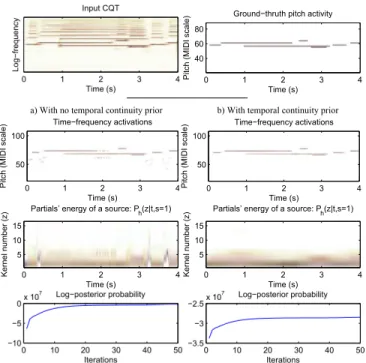
C. Spectral envelope temporal continuity prior

The HALCA model allows modeling notes with time-varying fundamental frequencies or spectral envelopes. But so far, nothing constrains those attributes to evolve smoothly over time, whereas it could be a useful piece of information, as usually observed in real-world musical sounds. Many solutions have been suggested in order to enforce temporal continuity whether in the framework of NMF or PLCA. One can mention for instance [3] or [16], where a smoothness constraint is imposed respectively via a penalty term in the NMF cost function and via a prior on the parameters in the framework of Bayesian NMF. In [8], the temporal continuity is imposed by applying a Kalman filter smoothing on the impulse distributions between two iterations of the EM algorithm. The common characteristic of most of the proposed methods for enforcing the continuity of spectrogram decomposition is that they enforce the temporal smoothness of the energy of the sources. The new idea here is instead to enforce the temporal continuity of the timbre of the sources, which in the HALCA model is represented by the envelope coefficients �ℎ(�♣�, �).

We use this constraint for several reasons. First, it can prevent the EM algorithm from staying stuck in a local maximum. Then, contrary to a prior of energy temporal smoothness, enforcing timbre temporal continuity does not disfavor hard attacks of notes. A more obvious reason is that we already introduced the sparse prior and the monomodal prior applied on the impulse distribution (sections IV-A and IV-B), and two different priors on the same set of parameters might lead to some difficulties, in terms of mathematic calculation.

For a given source �, let Θ and W respectively denote the

� × � matrix of coefficients ���= �ℎ(�♣�, �) and the � × �

matrix of coefficients �� � =

︀

�,��� �� (�, �, �, � = ℎ♣�, �).

We introduce a new prior on Θ, defined as:

� �(Θ) ∝ ︀ ︁ ︁ � � ︁ �=2 2 ︁ �� ���⊗1� �� �+ � �⊗1 � ︀ ︀ ä (26) where ä is a positive hyperparameter indicating the strength of the prior. Such a prior indeed favors slow evolution of the coefficients in each row of Θ, since the closer two numbers are, the bigger the ratio between their geometric and arithmetic means is. Maximizing

�Λ+ ln (� �(Θ)) w.r.t. Θ corresponds to maximizing the

function: � : Ω = ]0, 1[�×� ⊗⊃R Θ↦⊗⊃︁ � � ︁ �=1 ���log(���)+ ä︁ � � ︁ �=2 ln ︀ ︁ ︁ �� ���⊗1� �� �+ ���⊗1 ︀ ︀, (27)

under the constraint ∀ �,︀

����= 1. If ˆΘis the maximum

that we are looking for, then according to the KKT

conditions, ∀ � there exists a unique à�∈ R such that

∀� ⎧ ︁ ︁ ︁ ︁ ︁ ︁ ︁ ︁ ︁ ︁ ︁ ︁ ︁ ︁ ︁ ︁ ︁ ︁ ︁ ︁ ˆ ���= �� �+ ä à�+_2ˆä_�t z +_�ˆt+1ä z +ˆ�zt if � = 1 ˆ �� �= �� �+ ä à�+_�ˆt−1ä z +ˆ�tz +_�ˆt+1ä z +ˆ�tz if � ∈ J2, � ⊗ 1K ˆ ���= �� �+ ä à�+_�ˆt−1ä z +ˆ�tz + ä 2ˆ�t z if � = � . (28) Unfortunately, as for the monomodal prior, there is no closed form solution, and we cannot be sure that there is a unique solution. However, numerical simulations showed that the fixed point Algorithm 2 always converges to a solution that makes the posterior probability increase from one iteration of the EM algorithm to the next. Fig. 5 illustrates the use of the prior.

Algorithm 2: Fixed-point method for the temporal

continuity prior ∀ (�, �) ∈ J1, �K × J2, � K, ˆ�� �⊂ �t z ︀ ˜ z� t ˜ z ; repeat ≤ ∀ � ∈ J1, �K, �1 �⊂ ä/(2ˆ�1�) ; ≤ ∀ (�, �) ∈ J1, �K × J2, � K, �� �⊂ ä/(ˆ���⊗1+ ˆ���); ≤ ∀ � ∈ J1, �K, �� +1 � ⊂ ä/(2ˆ���);

≤ ∀� ∈ J1, � K, find the unique à�_{such that}

︀ � �t z+ä àt_+�t z+� t+1 z = 1 and ∀�, �t z+ä àt_+�t z+� t+1 z ⊙ 0 (we

used Laguerre’s method [30]); ≤ ∀ (�, �) ∈ J1, �K × J2, � K, ˆ�� �⊂ �t z+ä àt_+�t z+�t+1z ; untilconvergence ;

V. APPLICATION AND EVALUATION

A. Some useful remarks

1) Parameters initialization: As for many iterative

maximization algorithms, the way parameters are initial-ized has a very important effect on the convergence to a local maximum. After experimentation, the following recommendations can be provided:

∙ random initialization is not recommended,

∙ a good initialization of the impulse distribution is the

uniform distribution (�ℎ(�, �, �) = 1/(� × � × �)),

∙ envelope coefficients �_ℎ(�♣�, �) must be initialized

differently for the different sources �.

2) Defining the hyperparameters: Each prior mentioned

in section IV depends on one or more hyperparameter (for instance the hyperparameter Ñ in the case of the sparse prior). For now, no research has been made on how to automatically estimate their value, hence the need to manually predefine them. However, after experimentation, we noticed that a good way to avoid local minima was to increase the values of the hyperparameters from 0 to the predefined values during the first iterations of the EM algorithm. This strategy stands for the monomodal and the sparse priors. Concerning the temporal prior, the value of ä can be fixed from the first iteration.

Time (s) P itch (MI DI scale) Time−frequency activations 0 1 2 3 4 50 100 0 10 20 30 40 50 −3.5 −3 −2.5x 10 7 Iterations Log−posterior probability 0 10 20 30 40 50 −10 −5 0x 10 7 Iterations Log−posterior probabilityTime (s)

K

ernel

n

umber

(z) Partials’ energy of a source: Ph(z|t,s=1)

0 1 2 3 4 5 10 15 Time (s) Log− freq uency Input CQT 0 1 2 3 4

a) With no temporal continuity prior b) With temporal continuity prior

Time (s)

K

ernel

n

umber

(z) Partials’ energy of a source: Ph(z|t,s=1)

0 1 2 3 4 5 10 15 Time (s) P itch (MI DI scale) Time−frequency activations 0 1 2 3 4 50 100 Time (s) P itch (MI DI scale)

Ground−thruth pitch activity

0 1 2 3 4

40 60 80

Fig. 5. Illustration of the use of the temporal continuity prior

and the growth of the criterion over the iterations. The input signal corresponds to several notes of clarinet and horn. The HALCA model has been estimated with � = 2 sources. The time-frequency activations correspond to the summation over the sources of the

impulse distribution:︀

s�h(�, �, �). The monomodal prior is used in both cases.

B. Monopitch estimation

To evaluate the relevance of the HALCA model, it has first been tested on a task of monopitch estimation. The database used for the evaluation consists of 3307 isolated notes from the Iowa database [32]. It includes recordings of several instruments, playing over their full range, and with various play modes and nuances. The CQT of each audio file is computed as discribed in section II-A. It is then analyzed with two different versions of the HALCA algorithms, with a number of sources set to � = 1: one using the monomodal prior only (denoted �1⊗�), one using both the monomodal

and the temporal continuity priors (denoted �1⊗ ��).

The pitch is finally inferred for each time frame from the maximum of the impulse distribution �ℎ(�♣�, � = 1) and

associated to the closest MIDI note. The methods are compared with the YIN algorithm [33], available on the author’s website1_{, using 100ms time frames. The output}

of this algorithm is as well rounded to the closest MIDI pitch. Results are illustrated in Fig. 6. Several conclusions can be made from those results. First, we can see that our results are comparable to those of YIN algorithm, except for the oboe and the bassoon. Those two instruments have indeed very high spectral centroids, regardless of the pitch, and where YIN makes upper octave or twelfth errors, the HALCA model adapts itself to the spectral shapes. It is also shown that the addition of the temporal prior to the monomodal prior improves the performances for each instrument. Since the HALCA model seems to be

1

http://audition.ens.fr/adc/

relevant for any kind of instrument, it can now be applied to polyphonic music.

0 5 10

Piano Violin Cello Tuba Flute FrenchHorn

Viola DoubleBass

Clarinet_Trombone Sax OboeTrumpet BassClarinet Bassoon error rate (%) H 1−m (mean: 2.27%) H 1−mt (mean: 1.81%) YIN (mean: 2.69%)

Fig. 6. Simulation results: averaged error rates for each instrument of the database in a task of monopitch estimation. The error rate corresponds to the proportion of frames for which the MIDI pitch is wrongly estimated. The monomodal prior is used for both HALCA algorithms.

C. Automatic transcription

This section is dedicated to the application of the HALCA model to automatic music transcription. First, the complete transcription system is presented as well as the metrics used to assess its performance. Then, the model is tested on a first database, on which several versions of our algorithm are compared, including different sets of values for the hyperparameters and different values for the model order �. Finally, three versions of the HALCA model are compared to other state of the art transcription algorithms on a second database.

1) Description of the transcription system:

∙ For a given input audio signal, the CQT is first

calculated as described in section II-A.

∙ It is then analyzed with the HALCA algorithm and the

time-frequency activation matrix �ℎ(�, �) is deduced

from the estimated impulse distribution: �ℎ(�, �) =

︀

��ℎ(�, �, �).

∙ To obtain a pitch activity matrix �, �(�, �)

corre-sponding to the velocity of pitch � (integer on the MIDI scale) at time �, every peak of each vector (�ℎ(�, �))_� (� from 1 to � ) is first detected. Then, at

time �, a given peak �0is associated to the

correspond-ing nearest pitch number �0 and �(�0, �) is set to

�(�0, �) = �ℎ(�0⊗ 1, �) + �ℎ(�0, �) + �ℎ(�0+ 1, �). � is

then normalized as follows : � ⊂ �/ max�,��(�, �).

∙ Finally, onset/offset detection is employed to

tran-scribe note events. For each pitch �, an onset (resp. an offset) is detected as soon as �(�, �) becomes larger (resp. lower) than �min for more than 70ms, �min

being a fixed threshold. In order to consider onsets of repeating notes (i.e. when the energy of pitch � remains above the threshold �min whereas there is a

new onset), we applied another onset detection on the derivative �′_{(�, �) of �(�, �) w.r.t. time. A new onset}

is detected once �′_{(�, �) > �}′

min, �′minbeing another

fixed threshold. If two detected onsets of a same MIDI note are closer than 100ms, only the first one is kept.

2) Metrics: once for all A given estimated note is

considered to be correctly transcribed if a note with a same pitch and onset time (within 50 ms) can be found in the ground truth. Traditional measures of recall ℛ, precision � and F-measure ℱ [34] are then calculated to assess the performance.

3) Playing with the parameters on a training database:

Five 30 s excerpts from the RWC classical genre database [35], all listed in Tab. II (page 11) and referred to as database DB�����, were used for those preliminary

eval-uations.

As already mentioned in section III-A1, in practice, one source represents a “meta-instrument” rather than a real instrument. Consequently, there is no need to set the number of sources � to the actual number of instruments in the input signal: a fixed number of sources can be sufficient to model an unknown number of instruments. In order to both verify this statement and to find a good value for � (so that we can fix it once for all), in a first experiment, the proposed transcription algorithm has been performed using different values of � on each file of DB�����. In this

experiment, no prior was added and the onset detection thresholds ���� and �′��� have been optimally set for

each file and each value of �. Results are reported in Tab. III. For each file, by comparing the value of � which

S rwc(1) rwc(2) rwc(3) rwc(4) rwc(5) Mean 1 72.2 31.1 43.3 43.5 73.8 47.0 2 76.7 32.0 45.7 45.1 80.3 50.0 3 78.9 33.3 46.0 _{45.4 80.7 50.5} 4 81.4 33.1 45.7 45.8 _81.5 51.1 5 82.0 _{32.3 46.0 45.3} 82.2 _50.7 6 82.0 32.7 47.1 45.2 82.2 51.0 TABLE III

Study of the influence of the value of �: F-measure for each

file of DBtrainwhen onset thresholds are optimally set.

maximizes the performance, and the effective number of instruments (see Table II), one can observe that there is no correlation between those two quantities. Indeed, best results are always given for � between 3 and 5, regardless of the number of instruments. We can then conclude that setting � to a fixed value can be sufficient to model any number of instruments and that it will not have a negative effect onto the transcription performance. From now on, � is fixed to 4, which is the best value in this first experiment, in terms of mean results.

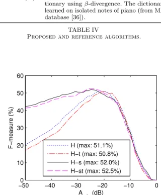
The aim of the second test is to evaluate the influence of the use of the different priors on the transcription system. To do so, four different systems, all described in Tab. IV, have been evaluated on this database: �4 will refer to

the basic model with no prior, �4⊗ � to the system with

the temporal prior alone, �4⊗ � to the system with the

sparse prior alone, and finally �4⊗ �� with both priors.

The subscript 4 means that the number of sources is

� = 4. From experiments that we performed on this same

database, hyperparameters Ñ and ä have been manually set to optimal values, as well as the onset threshold �′

���.

Results are showed in Fig 7, where the average F-measure w.r.t. the onset threshold ���� is plot for each system. A

Symbol Description

�4 HALCA model with no prior.

�4⊗ � HALCA model with spectral envelope temporal

continuity prior.

�4⊗ � HALCA model with sparseness prior.

�4⊗ �� HALCA model with spectral envelope temporal

continuity and sparseness priors.

Vincent’10 [13] Multiplicative NMF with the Ñ-divergence (Ñ =

0.5) and harmonicity and spectral smoothness constraints.

Dessein’12 [10] Spectrogram decomposition on a learned

dic-tionary using Ñ-divergence. The dicdic-tionary is learned on isolated notes of piano (from MAPS database [36]).

TABLE IV

Proposed and reference algorithms.

−500 −40 −30 −20 −10 0 10 20 30 40 50 60 A min (dB) F−measure (%) H (max: 51.1%) H−t (max: 50.8%) H−s (max: 52.0%) H−st (max: 52.5%)

Fig. 7. Study of the influence of the different priors: average

F-measure w.r.t. �minfor four versions of the proposed transcription system.

first remark is that the system seems to behave similarly whether the spectral envelope temporal continuity prior is active or not, even though this prior does affect the estimation of the parameters (see for instance Fig. 5). One explanation could rely in the post-processing stage for the automatic transcription (the calculation of the resulting pitch activity matrix �(�, �) as well as the onset/offset detection) which seems to smooth the lack of temporal continuity when the prior is not used. We can also wonder why the continuity prior did have a clear positive impact on the monopitch evaluation. It appears that the monomodal prior makes the algorithm more sensitive to local maxima (basically it can lead to octave errors). The role of the continuity prior is then to avoid those local minima. When no monomodal prior is used, as in this experiment, the role of the continuity prior is thus weakened. It can be noticed though that on this database, it slightly improves the maximum F-measure, when combined to the sparse prior. Concerning this last prior, its effect can be clearly seen: besides increasing the maximal value of ℱ, it allows

Symbol Title (Composer) Catalog number # of instruments Pol. level (Ave. / Max.)

rwc(1) The Musical Offering (Bach) RWC-MDB-C-2001 No. 12 2 1.3 / 4

rwc(2) String Quartet No. 19 (Mozart) RWC-MDB-C-2001 No. 13 4 2.7 / 5

rwc(3) Clarinet Quintet Op.115. (Brahms) RWC-MDB-C-2001 No. 17 5 3.8 / 10

rwc(4) Horn Trio Op.8 (Brahms) RWC-MDB-C-2001 No. 18 3 4.2 / 10

rwc(5) The Anna Magdalena Bach Notebook (Bach) RWC-MDB-C-2001 No. 24a 1 1.9 / 5

TABLE II

DBtrain: list of the audio excerpts from RWC classical genre database [35] and their corresponding number (#) of sources and polyphony (Pol.) level.

the system being a lot less sensitive to a suboptimal value of ����. Since the optimal threshold might change

according to the file or the database, this characteristic is quite interesting. From those preliminary results it is possible to determine good values of the fixed parameters for each version of the HALCA algorithm. Those values are summarized in Tab. V. It can be noticed that the chosen thresholds ���� are slightly lower than the ones

that maximize ℱ on DB�����. The reason is that the

F-measure curves decrease faster if ���� is overestimated

than if it is underestimated. Doing so, we hope that the proposed algorithms will be more robust to the nature of the evaluation dataset. Only the three systems H, �4⊗ �

and �4⊗�� are kept for comparison with other transcription

algorithms from the literature.

System S �min(��) �′_min Ñ ä

�4 4 -25 0.018 0 0

�4⊗ � 4 -30 0.018 0.06 0

�4⊗ �� 4 -30 0.018 0.06 107

TABLE V

Value of the fixed parameters for the proposed algorithms.

4) Comparing with other methods on an evaluation database: In order to compare the performance of the

two systems �4⊗ � and �4⊗ �� to other state-of-the-art

al-gorithms, a second database denoted DB����and composed

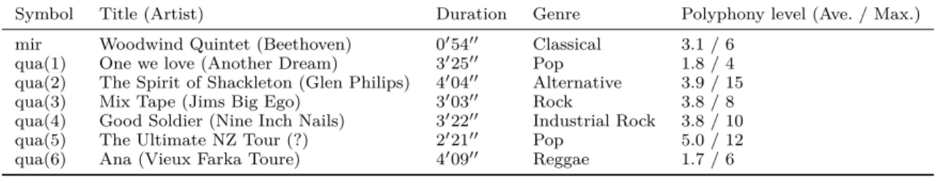
of 7 audio files has been set up. The first file of DB����

is a 54 s excerpt from a woodwind quintet transcription of Beethoven’s string quartet No.4 Op.18, available in the MIREX 2007 multi-F0 development dataset [37]. The other recordings are from the QUASI transcription corpus [38]. Each file is briefly described in Tab. VI (page 12).

The performance of the algorithms �4⊗ � and �4⊗ ��

are compared with two other NMF based transcription systems, namely Vincent’10 [13] and Dessein’12 [10] all described in Tab. IV. Those systems are run from their author’s implementation, which they kindly shared. Global transcription results (ℱ) for each file of DB����are reported

in Tab. VII whereas mean transcription metrics and computation time2 are reported in Tab. VIII. From those tables, several interesting results can be pointed out. First, the same conclusion as in section V-C3 can be drawn: 2_{Evaluations have been done using a 64-bit version of Matlab on a}

3.1GHz processor.

File �4 �4⊗ � �4⊗ �� Vincent’10 Dessein’12

mir 62.0 _{58.8 60.8 57.9 52.0} qua(1) 34.3 40.8 41.8 _{10.0 19.0} qua(2) 15.8 16.7 _{15.6 8.4 7.8} qua(3) 11.1 _{9.5 9.0 6.8 2.5} qua(4) 19.6 27.6 _{27.0 8.0 13.6} qua(5) 18.3 16.6 18.5 _{9.8 13.7} qua(6) 47.9 _{46.9 46.4 9.5 4.3} mean 29.9 31.0 31.3 _{15.8 16.1} TABLE VII

Transcription results: F-measure (%) for each file of DBeval.

Algorithm ℱ (%) ℛ(%) � (%) CT ( × real time)

�4 29.9 27.9 37.0 3.4 �4⊗ � 31.0 26.6 40.3 4.3 �4⊗ �� 31.3 27.6 38.6 7.5 Vincent’10 15.8 48.0 _{10.6 0.9} Dessein’12 16.1 20.1 14.9 0.8 TABLE VIII

Mean results and computation time (CT) on DBeval.

results from the two systems �4⊗ � and �4⊗ �� are very

similar and the addition of the temporal prior does not significantly improve the performances of the transcription system. Concerning the use of the sparse prior, it can be seen that it slightly improves the global F-measure. In any case, the algorithms we provide have the best F-measure for each file of DB����, and therefore the best

average F-measure. One interesting characteristic can be deduced from Tab. VII: the relative difference between the performance of H, �4⊗ � or �4⊗ �� and the performance

of Vincent’10 or Dessein’12 is much greater for the files of QUASI corpus (qua(n)) than for the Mirex woodwind quartet (mir). This highlights the relative robustness of the proposed model to the musical genre. The conclusion one can draw from Tab. VIII is that each transcription system would benefit from including an automatic estimation of the threshold of note detection (���� in our case). In fact,

the difference between ℛ and � can teach us that this threshold is not optimal for each file of DB����, whereas it

has been set so that it is optimal on some other dataset (DB����� in our case).

Symbol Title (Artist) Duration Genre Polyphony level (Ave. / Max.)

mir Woodwind Quintet (Beethoven) 0′₅₄′′ _{Classical 3.1 / 6}

qua(1) One we love (Another Dream) 3′₂₅′′ _{Pop 1.8 / 4}

qua(2) The Spirit of Shackleton (Glen Philips) 4′₀₄′′ _{Alternative 3.9 / 15}

qua(3) Mix Tape (Jims Big Ego) 3′₀₃′′ _{Rock 3.8 / 8}

qua(4) Good Soldier (Nine Inch Nails) 3′₂₂′′ _{Industrial Rock 3.8 / 10}

qua(5) The Ultimate NZ Tour (?) 2′₂₁′′ _{Pop 5.0 / 12}

qua(6) Ana (Vieux Farka Toure) 4′₀₉′′ _{Reggae 1.7 / 6}

TABLE VI

DBeval: list of the audio excerpts from MIREX 2007 multi-F0 development dataset [37] and QUASI transcription corpus [38].

VI. CONCLUSION

In this paper, we proposed a new PLCA-based model called HALCA which analyzes harmonic structures in musical signals. The model does not rely on an hypothesis of redundancy, and therefore is quite expressive. Particu-larly, it allows modeling sources that have both temporal variations of pitch and spectral envelope. The presence of noise is also considered in order to enforce the robustness of the model to real data. Three new priors that help the algorithm to converge toward a meaningful solution have also been proposed. Those priors are generic and can be applied to any other PLCA-based model. The HALCA model has first been tested on a task of monopitch estimation and the results have showed that it could fit to many kinds of musical instruments. Then, it has been tested on a task of automatic transcription on two different databases. On the training one, the effect of using the different priors has been studied. It appeared that the use of the sparse prior has an impact on the sensitivity to the onset detection threshold. On the contrary, the use of the timbre temporal continuity does not seem to significantly improve the results in this task of automatic transcription. The training database is also used to fix the hyperparameters of the system. On the second database, three versions of the HALCA algorithm are compared to two state-of-the-art algorithms. The results our systems provide and their comparison with the reference systems permit to outline the following conclusions. First, even if the addition of a sparse prior can improve the performance of a threshold-based onset detection, we think that every system would benefit from being able to automatically estimate this threshold w.r.t. the input signal. In future work, we plan to imagine a model where the sparse prior is replaced by the estimation of the best onset detection threshold. The second conclusion is that maybe the hypothesis of redundancy is not necessary for a TFR factorization technique to be efficient, and a highly expressive model is recommended to be robust to any kind of real musical signal.

The Matlab implementation of the algorithm can be found online : http://www.tsi.telecom-paristech.fr/aao/en/ 2012/07/13/fuentes2012_ieee/.

Appendix A

EM update rules with sparse prior

One want to find the argument ˆθ _{of the maximum of}

the function � defined in (24) under the constraint �(θ) =

1 ⊗︀

��� = 0. We know that the maximum exists since

� is bounded on Ω and that it verifies first and second

order necessary conditions, proper to local minima (� and

� are twice differentiable): there exists an unique � ∈ R

such that (⟨., .⟩ denotes the scalar product)

∇��( ˆθ) = 0 and (29) ︀ �︁��( ˆθ) ⎡ �, �︁⊘ 0, � ∈︁� ∈ R�/⟨∇�( ˆθ_{), �⟩ = 0}︁_, (30) where �� is the Lagrange function defined as:

�� : Ω ⊗⊃ R

θ_{↦⊗⊃ �(θ) + � �(θ),} (31)

and where �︁��( ˆθ)

⎡

is the Hessian matrix of �� at point

ˆ

θ_{. Equation (29) leads to:}

∀�, �_ˆ� �� ⊗Ñ √ � ︁ ˆ �� ⊗ � = 0. (32) If � = 0, then ∀�, ˆ��= ��2 Ñ2_� (33)

which is possible only if︀

� �2 j Ñ2_� = 1. If � > 0, then ∀�, ︁ ˆ ��= ⊗Ñ √ � +︀Ñ2_{� + 4��} � 2� that is to say: ∀�, ˆ��= 2�2 � �Ñ2_{+ 2��} �+ Ñ √ �︀Ñ2_{� + 4��} � , (34)

which is possible only if ︀

� �2

j

Ñ2_� > 1. In this case, we can prove that there is a unique � > 0 such that︀

��ˆ�= 1. If max�⊗Ñ 2_� 4�j ⊘ � < 0, then, ∀�, ˆ��= 2�2 � �Ñ2_{+ 2��} �∘ Ñ √ �︀Ñ2_{� + 4��} � , (35) which leads to 2� _{possible solutions. However, if we take a}

vector � such that ⎧ ︁ ︁ ︁ ︁ ��1= 1, �1∈ J1, �K ��2= ⊗1, �2∈ J1, �K \ ¶�1♢ ��= 0, ∀� ∈ J1, �K \ ¶�1, �2♢ ,