HAL Id: hal-01070496
https://hal-onera.archives-ouvertes.fr/hal-01070496
Submitted on 1 Oct 2014
HAL is a multi-disciplinary open access
archive for the deposit and dissemination of
sci-entific research documents, whether they are
pub-lished or not. The documents may come from
teaching and research institutions in France or
abroad, or from public or private research centers.
L’archive ouverte pluridisciplinaire HAL, est
destinée au dépôt et à la diffusion de documents
scientifiques de niveau recherche, publiés ou non,
émanant des établissements d’enseignement et de
recherche français ou étrangers, des laboratoires
publics ou privés.
Pattern classification with missing data using belief
functions
Z. Liu, Q. Pan, G. Mercier, J. Dezert
To cite this version:
Z. Liu, Q. Pan, G. Mercier, J. Dezert. Pattern classification with missing data using belief functions.
Fusion 2014, Jul 2014, SALAMANCA, Spain. �hal-01070496�
Pattern classification with missing data
using belief functions
Zhun-ga Liu
a,b, Quan Pan
a, Gregoire Mercier
b, Jean Dezert
ca. School of Automation, Northwestern Polytechnical University, Xi’an, China. Email: [email protected] b. Telecom Bretagne, CNRS UMR 6285 Lab-STICC/CID, Brest, France, Email: [email protected]
c.ONERA - The French Aerospace Lab, F-91761 Palaiseau, France. Email: [email protected]
Abstract—The missing data in incomplete pattern can have different estimations, and the classification result of pattern with different estimations may be quite distinct. Such uncertainty (ambiguity) of classification is mainly caused by the loss of information in missing data. A new prototype-based credal classification (PCC) method is proposed to classify incomplete patterns using belief functions. The class prototypes obtained by the training data are respectively used to estimate the missing values. Typically, in a c-class problem, one has to deal with c prototypes which yields c estimations. The different edited patterns based on each possible estimation are then classified by a standard classifier and one can get c classification results for an incomplete pattern. Because all these classification results are potentially admissible, they are fused altogether to obtain the credal classification of the incomplete pattern. A new credal combination method is introduced for solving the classification problem, and it is able to characterize the inherent uncertainty due to the possible conflicting results delivered by the different estimations of missing data. The incomplete patterns that are hard to correctly classify will be reasonably committed to some proper meta-classes by PCC method in order to reduce the misclassification rate. The use and potential of PCC method is illustrated through several experiments with artificial and real data sets.
Index Terms—belief functions, evidence theory, missing data, data classification, fusion rule
I. INTRODUCTION
The classification of incomplete patterns with missing val-ues is an important topic in the field of machine learning. There have been many methods [1] emerged for classifying incomplete patterns, and it mainly concerns the handling miss-ing values and pattern classification. The simplest method just deletes the incomplete patterns [2], and the classifier is applied only for the complete patterns. The model of probability density function (pdf) of the whole data set is also sometimes derived for the classification based on the Bayes decision theory [3]. Some classifiers [4] particularly designed for deal-ing with the incomplete data without estimation of missdeal-ing values have also been developed. The imputation strategy [5] is often adopted for missing values in many cases, and then the edited patterns with estimated values are classified. A number of methods have been introduced for imputation of missing values, and they can be generally grouped into two types [1]. One type is statistical analysis imputation methods including mean imputation, regression imputation, multiple imputation, hot deck imputation, and so on. Particularly, in the mean
imputation (MI) method [6], the missing values are replaced by the mean of known values of that attribute. Another type is imputation methods based on machine learning, it includes the K-nearest neighbor imputation (KNNI) and SOM imputation, etc. In the often used KNNI method [7], the missing values are estimated using the K-nearest neighbors of the object (incomplete pattern).
The missing data can have several different possible esti-mated values, and the classification result of the incomplete pattern (test sample) with different estimations can be very different sometimes. For example, an object using a given estimation of missing data can be classified into the class A with biggest probability, but it could also be most likely classified into the class B, with A ∩ B = ∅ using another given estimation of missing data. Such conflict (uncertainty) of classification is caused by the lack of information of the missing (unknown) values, and it is really hard to correctly classify the object in such condition because the known (avail-able) attributes information is really insufficient for making a specific classification. The belief function framework intro-duced by Shafer [8]–[10] in Dempster-Shafer theory (DST) is appealing for dealing with such uncertain and imprecise infor-mation [11]. Belief functions have been already used in many fields, such as data classification [12]–[16], data clustering [17]–[20], and decision-making [21]. Some data classification methods [16] have been developed based on DST. A K-nearest neighbors rule based on DST is proposed in [13], and a neural network classifier working with DST is presented in [14]. In the aforementioned methods, the meta-classes defined by the disjunction of several specific classes (i.e. the partially ignorant classes) are not considered as potential solutions of the classification. In our very recent work, a new belief K-nearest neighbor (BK-NN) classifier [15] working with credal classification has been presented to deal with uncertain data by considering all possible meta-classes in the classification process because the meta-classes are truly useful and important to represent the imprecision of the classification. Nevertheless, these classification methods working with belief functions were all designed for classifying complete patterns only, and the missing data aspect was not taken into account.
In this work, a new prototype-based1 credal classification
1The estimation of missing data in this new method is based on the
(PCC) method is proposed for the classification of incomplete patterns under belief function framework. The object hard to correctly classify due to the uncertainty (imprecision) caused by the missing values will be reasonably committed to the proper meta-class defined by the union (disjunction) of several specific classes (e.g.A ∪ B) that the object likely belongs to. This approach allows us to both reduce the misclassification error rate, and to reveal the imprecision of the classification. This paper is organized as follows. After a brief introduction of the basics of evidential reasoning in section II, the new prototype-based credal classification method is presented in the section III. The proposed method PCC is then tested in section IV and compared with two other classical methods, followed by conclusions.
II. BRIEF RECALL OF EVIDENCE THEORY
The belief functions have been introduced by Shafer in his original Mathematical Theory of Evidence [8]–[10]. This theory is also known classically as Evidential Reasoning (ER) approach, or also as Dempster-Shafer Theory (DST). In this theory, one starts with a frame of discernment Ω = {ω1, . . . , ωi, . . . , ωc} consisting of a finite discrete set of
mutu-ally exclusive and exhaustive hypotheses (classes). The power-set of Ω, denoted 2Ω
, is the set of all the subsets of Ω. For example, ifΩ = {w1, w2, w3}, then 2Ω= {∅, ω1, ω2, ω3, ω1∪
ω2, ω1∪ω3, ω2∪ω3, Ω}. The singleton class (e.g. ωi) is called a
specific class. The disjunctions (union) of several single classes that represent the partial ignorances in 2Ω (e.g. ω
i∪ ωj, or
ωi∪ ωj∪ ωk, etc) are called meta-classes.
A basic belief assignment (BBA) is a functionm(.) from 2Ω
to[0, 1] satisfying ∑
A∈2Ω
m(A) = 1 and m(∅) = 0. The subsets A of Ω such that m(A) > 0 are called the focal elements of m(.). The credal classification (partition) [17], [18] is defined asn-tuple M = (m1, · · · , mn), where mi is the basic belief
assignment of the object xi ∈ X, i = 1, . . . , n associated with
the different elements of the power-set2Θ
. The mass of belief of meta-class can well reflect the imprecision (ambiguity) degree of the classification of the uncertain data. The lower and upper bounds of imprecise probability associated with BBAS correspond to the belief function Bel(.) and the plausibility functionP l(.) [8]. They are given for all A ∈ 2Ω
by Bel(A) = ∑ B⊆A m(B) (1) P l(A) = ∑ B∩A̸=∅ m(B) (2)
Bel(.) and P l(.) can be used for decision-making support when adopting pessimistic or optimistic attitudes if necessary. In DST framework, Shafer proposed that the different pieces of evidence represented by BBAS should be combined using Dempster’s rule [8], commonly denoted DS rule in the literature and represented by ⊕ symbol. Mathematically, DS rule of combination of two BBASm1(.) and m2(.) defined on
2Θ is defined by m DS(∅) = 0 and for A ̸= ∅, B, C ∈ 2Θ by mDS(A) = [m1⊕ m2](A) = ∑ B∩C=A m1(B)m2(C) ∑ B∩C̸=∅ m1(B)m2(C) (3)
In DS rule, the total conflicting belief mass is redistributed back to all the focal elements through a classical normaliza-tion step. However, it is known that DS rule produces very unreasonable results not only in the high conflicting cases, but also in some very special low conflicting cases as well [23], [24], and that is why many other combination rules [25] have been developed to overcome its limitations.
III. NEW METHOD FOR CLASSIFICATION OF INCOMPLETE PATTERNS
The new prototype-based credal classification (PCC) method provides multiple possible estimations of missing values according to class prototypes obtained by the training samples. For a c-class problem, it will produce c probable estimations. The object with each estimation is classified using any standard2 classifier. Then, it yields c pieces of
classification results, but these results take different weighting factors depending on the distance between the object and the corresponding prototype. So thec classification results should be discounted with different weights, and the discounted results are globally fused for the credal classification of the object. If thec classification results are quite consistent on the decision of class of the object, the fusion result will naturally commit this object to the specific class that is supported by the classification results. However, it can happen that high conflict among thec classification results occurs which indicates that the class of this object is quite imprecise (ambiguous) only based on the known attribute values. In such conflicting case, it becomes very difficult to correctly classify the object in a particular (specific) class, and it becomes more prudent and reasonable to assign the object to a meta-class (partial imprecise class) in order to reduce the misclassification rate. By doing this, PCC is able to reveal the imprecision of the classification due to the missing values which is a nice and useful property. Indeed in some applications, specially those related to defense and security (like in target classification) the robust credal classification results are usually more preferable than the precise classification results subject potentially to a high risk of error. The classification of the uncertain object in meta-class can be eventually precisiated (refined) using some other (costly) techniques or with extra information sources if it is really necessary. So PCC approach prevents us to take erroneous fatal decision by robustifying the specificity of the classification result whenever it is necessary to do it.
A. Determination ofc estimations of missing values in
incom-plete patterns
Let us consider a test data set X = {x1, . . . , xN} to be
classified using the training data setY = {y1, . . . , yH} in the
frame of discernmentΩ = {ω1, . . . , ωc}. Because we focus on
the classification of the incomplete data (test sample) in this work, one assumes that the test samples are all incomplete data (vector) with single or multiple missing values, and the training data setY consists of a set of complete patterns.
The prototype of each class i.e.{o1, . . . , oc} is calculated
using the training data at first, and og corresponds to class
ωg. There exists many methods to produce the prototypes. For
example, the K-means method can be applied for each class of the training data, and the clustering center is chosen for the prototype. The simple arithmetic average vector of the training data in each class can also be considered as the prototype, and this method is adopted here for its simplicity. Mathematically, the prototype is computed forg = 1, . . . , c by
og= 1 Tg ∑ yj∈ωg yj (4)
whereTg is the number of the training samples in the class
ωg.
Once each class prototype is obtained, we use the value of the prototype to fill the missing values of the object (incomplete pattern) in the same attribute dimension. Because one has considered c possible classes with their prototypes, one getsc versions of estimated values for the object. For the object xiwith some unknown (missing) component values, the
c versions of estimations of the missing component values xij
of xi are given by
xgij = ogj (5)
where ogj is the j-th component of the prototype og, g =
1, 2, . . . , c.
From each complete estimated vector xgi, g = 1, 2 . . . , c, we can draw a classification result using any standard classifier working with the complete pattern. At this step, the choice of the classifier, denoted Γ(.), is left to user’s preference. For instance, one can use for Γ(.) the artificial neural network (ANN) approach, or the EK-NN, etc. The c pieces of sub-classification results for xi are given forg = 1, . . . , c by
Pgi = Γ(xgi|Y ) (6) where Γ(.) represents the chosen classifier, and Pgi is the output (i.e. classification result) of the classifier when using the prototype of classωg to fill the incomplete pattern xi. Pgi
can be a Bayesian BBA if the chosen classifier works under probability framework (e.g. K-NN, ANN), and it can also be a regular BBA with having some mass of belief committed to the ignorant classΩ if the classifier works under belief functions framework (e.g. EK-NN).
In this new PCC approach, we propose to combine these c pieces of classification results in order to get a credal classification of the incomplete pattern to classify. These c pieces of classification results are considered as c distinct sources of evidences. Because the distances between the object and the c prototypes are usually different, some discounting technique must be applied to weight differently the impact of these sources of evidences in the global fusion process. If the distance of the object to prototype is big according to
the known attribute values, it means that the estimation of the missing values using this prototype is not very reliable. So the bigger distancedijusually leads to the smaller discounting
factorαj. A rational way that has been widely applied in many
works is adopted here to estimate at first the weighting factor wgi. Forg = 1, . . . , c, this factor wgi is defined by
wig= e−dig (7) where dig= v u u t 1 p p ∑ s=1 ( xis− ogs δgs )2 (8) with δgs= √ 1 Tg ∑ yi∈ωg (yis− ogs) 2 (9)
xis is value of xi in s-th dimension, and yis is value of yi
in s-th dimension. p is the number of dimensions of known values of xi. The coefficient 1/p is necessary to normalize
the distance value because each test data can have a different number of dimensions of missing values. δgs is the average
distance of all training data belonging to class ωg to the
prototype og in s-th dimension, and it is introduced mainly
for dealing for the anisotropic data set. Tg is the number of
training samples in the class ωg.
From these weighting factorswgi forg = 1, . . . , c, one then defines the relative reliability factors (discounting factor) αgi by αgi = w g i wmax i (10) wherewmax i = max(w1i, . . . , wci).
The discounting method proposed by Shafer in [8] is applied here to discount the BBA of each source of evidence according to the factors αgi. More precisely, the discounted masses of belief are obtained forg = 1, . . . , c by
{ mgi(A) = αs iP g i(A), A ⊂ Ω mgi(Ω) = 1 − αgi + αigPig(Ω) (11) In Eq. (11), the focal element A usually represents a specific class in Ω because most classical classifiers work with probability framework only, and thus they just consider specific classes as an admissible solution of the classification. Nevertheless, some classifiers based on DST, like EK-NN, can generate results on specific classes and also on the full ignorant class Ω as well. Pig(A) is the probability (or belief mass) committed to the classA by the chosen classifier.
B. Fusion of thec discounted classification results
Thec classification results obtained according to the c pro-totypes may strongly support different classes that the object should belong to. For instance, several sources of evidence could strongly support that the object is most likely in class A, whereas some others could support strongly the class B, withA∩B = ∅. In practice, some conflict usually exists in the
global fusion process. The maximum of belief functionBel(.) given in Eq. (1) is used as criteria3 for the decision making
of the class which is strongly supported by the classification results, and thec pieces of results can be divided into several distinct groups G1, G2, . . . , Gr according to the classes they
strongly support.
The classification results in the same group are combined at first, and then these sub-combination results are globally fused for the credal classification. The classification results in the same group are generally not in high conflict. Therefore, one proposes to apply DS rule (3) to fuse these results, since DS rule offers a reasonable compromise between the specificity of the result and the level of complexity of the combination.
ForGs = {mji, . . . , mki}, the fusion results of the BBAS
in the group Gs using DS rule are given for a focal element
A ∈ 2Ω by: mωs i (A) = [m j i ⊕ . . . ⊕ m k i](A) (12)
where ⊕ represents the DS combination defined in Eq. (3). Since DS rule is associative, these BBAS can be combined sequentially using eq. (3) and the sequential order doesn’t matter.
These sub-combined BBAS mωs
i (.), for s = 1, . . . , r, will
then be globally fused to get the final BBA of the credal clas-sification. In the global fusion process, these sub-combination results of the different groups of sub-classification results can be in high conflict because of the distinct classes they strongly support according to their belief functions. Because DS rule is known to produce counter-intuitive results specially in high conflicting situations [26] due to its way of redistributing the conflicting beliefs, we propose to use another fusion rule to circumvent this problem. We recall that in DS rule the conflicting masses of belief are redistributed to all focal elements by the classical normalization step of Eq. (3). In our context, the partial conflicting information are very important to characterize the degree of uncertainty and imprecision of the classification caused by the missing values, and they should be preserved and transferred to the corresponding meta-classes specially in the high conflicting situation. But if all the partial conflicts are always unconditionally kept in the fusion results, they generate a high degree of imprecision of the result which is not an efficient solution of the classification. To avoid this drawback, in the PCC approach we make a compromise between the misclassification error rate and the imprecision degree we want to tolerate. This compromise is obtained by selecting the conflicting beliefs that need to be transferred to the corresponding meta-classes. The selection is done conditionally and according to the current context following the method explained in the sequel.
For simplicity and notation convenience, we assume that the resulting sub-combined BBA of group Gs is focused on
the the classωs. That is Belωis(ωs) = max(Belωis(.)) where
Belωs
i (.) is computed from the BBA m ωs
i (.) thanks to Eq. (1),
3The plausibility function P l(.) can also be used here, since Bel(.) and
P l(.) have a straight corresponding relationship in such particular BBAS structure.
for s = 1, . . . , r. This indicates that ωs is strongly supported
by the BBAS in group Gs. Moreover, the class ωmax is the
most believed class of the object if one has Belωmax
i (ωmax) = max(Beliω1(ω1), . . . , Belωig(ωg)) (13)
We remind thatωmaxis the class having the biggestBel(.)
value among all the classification groups, whereas ωs, s =
1, . . . , g just takes the biggest Bel(.) value in the group Gs.
In practice however, it can happen that the beliefBelωs
i (ωs) of
the strongest class of the groupGscan be very close (or equal)
toBelωmax
i (ωmax) but ωscan be different ofωmax. When such
case occurs, the object can potentially belong to the other class ωs with a high likelihood. So we must consider all the very
likely specific classes as potential solution of the classification of the object xi. The set of these potential classes is denoted
Λi and it is defined by
Λi= {ωs|Belωimax(ωmax) − Beliωs(ωs) < ϵ} (14)
whereϵ ∈ [0, 1] is a chosen threshold. Because all classes in Λi
can very likely correspond to the real (unknown) class of xi,
they appear not very distinguishable according to the choice of the thresholdϵ. This means that a strategy of classification of the object xi based only on one specific class of Λi is
very risky because all elements of Λi must be considered as
acceptable in fact. To reduce misclassification errors with such type of strategy, we propose to keep all the subsets of Λi in
the fusion process and we deal with the involved meta-class. If the beliefs of the other classes (e.g. ωf)
are all much smaller than Belωmax
i (ωmax) as
Belωmax
i (ωmax) − Belωif(ωf) > ϵ, it means that the
class ωmax is generally distinct for the object with respect
to the other classes (e.g. ωf). Then, there is no necessity to
keep the meta-class, and one can just use the specific classes in such case.
The global fusion rule for these sub-combination results is defined by: ∀Bi⊆ Ω ˜ mi(A) = for A ∈ Ω with|A| = 1, or A = Ω ∑ r ∩ g=1 Bg=A mω1 i (B1) · · · mωir(Br),
for A ⊆ Λi, with |A| ≥ 2
∑ |A|∩ i=1 Bi=∅ |A|∪ i=1 Bi=A [mω1 i (B1) · · · mωis(Bs) r ∏ g=|A|+1 mωg i (Ω)] (15) In Eq. (15), r is the number of the groups of the clas-sification results. |A| is the cardinality of the hypothesis A, and it is equal to the number of singleton elements included in A. For example, if A = ωi ∪ ωj, then |A| = 2. The
conjunctive combination, which corresponds to the consensus of sub-combination results, is used in the first part of formula to calculate the mass of belief of the specific classes and of
the ignorant class4. In the second part of Eq. (15), the partial conflicting beliefs are committed to the selected meta-classes to reflect the imprecision degree of classification of the object with the specific classes included in the meta-class.
Because not all partial conflicting masses of belief are transferred into the meta-classes through the global fusion formula (15), the combined BBA is normalized as follows before making a decision:
mi(A) = ˜ mi(A) ∑ Bj ˜ mi(Bj) (16)
The credal classification of the object can be made directly based on this final normalized combined result BBAS, and the object will be assigned to the focal element (a class or a meta-class) with maximal mass of belief. The maximum of beliefBeli(.) of the singleton (specific) class, or the maximum
of plausibilityP li(.), or the maximum of pignistic probability
BetPi(.) drawn from the global combined BBA mi(.) are
usu-ally used as the criteria for making hard classification, but the hard classification is not recommended in such uncertain case. The credal classification based on the BBAS is preferred here since it can well reflect the inherent imprecision (ambiguity) degree of the classification due to the missing values. Guideline for choosing the meta-class threshold ϵ: In the applications, the threshold ϵ of PCC must be tuned according to the number of objects in meta-class. A small ϵ value generally leads to fewer objects in meta-classes, but it may cause more misclassifications for the uncertain objects. A big ϵ value yields more objects in meta-class and leads to higher imprecision degree, which is not an efficient solution for the classification. Soϵ should be tuned according to the imprecision degree of the fusion results that one accepts. The following simple example shows how PCC works. Example 1: Let us consider a 3-D object xi= [xi1, ?, ?] with
the missing value in the 2nd dimension and 3rd dimension to be classified over the frame of classes Ω = {ω1, ω2, ω3}. It
is assumed that the prototypesO = {o1, o2, o3} of the three
classes can be calculated using the training data as: o1= [o11, o12, o13]
o2= [o21, o22, o23]
o3= [o31, o32, o33]
So the object with three versions of estimation of the missing value is obtained by:
x1i = [xi1, o12, o13]
x2i = [xi1, o22, o23]
x3i = [xi1, o32, o33]
The patterns with three estimated values are respectively clas-sified using a standard classifier, and the classification results
4The ignorant class represents the outlier (noisy) class.
represented by the probability membership are given by: Pi1(ω1) = 0.8, Pi1(ω2) = 0.2
P2
i(ω1) = 0.1, Pi2(ω2) = 0.8, Pi2(ω3) = 0.1
P3
i(ω1) = 0.5, Pi3(ω2) = 0.2, Pi3(ω3) = 0.3
The relative weighting factor of each classification result is calculated according to the distance between xi and the three
prototypes using Eq. (10). For simplicity and convenience, they have been randomly chosen as follows for this example:
α1
i = 1, α2i = 0.9, α3i = 0.3
Then, each classification result Pk
i(.), k = 1, . . . , 3 can be
discounted using Eq. (11), and the discounted BBAS are given by m1 i(ω1) = 0.8, m1i(ω2) = 0.2 m2i(ω1) = 0.09, m2i(ω2) = 0.72, m2i(ω2) = 0.09, m2i(Ω) = 0.1 m3 i(ω1) = 0.15, m3i(ω2) = 0.06, m3i(ω3) = 0.09, m3i(Ω) = 0.7
Because of the particular choice ofα1
i = 1 the BBA m1i(.) is
not discounted in this example.
The belief functions Beli(.) corresponding to each BBA
mi(.) are obtained using Eq. (1) and are given by
Bel1 i(ω1) = 0.8, Bel1i(ω2) = 0.2 Bel2 i(ω1) = 0.09, Beli2(ω2) = 0.72, Bel2i(ω3) = 0.09 Bel3 i(ω1) = 0.15, Beli3(ω2) = 0.06, Bel3i(ω3) = 0.09
For the singleton (specific) class,m1
i(.) and m3i(.) put the most
belief on class ω1, whereas m2i(.) commits most of mass to
the classω2. It means that the object likely belongs to classω1
with the estimation from prototype o1 and o3, but it is very
probably classified into ω2 with the estimation according to
o2. This uncertainty (conflict) is mainly caused by the lack of
discriminant information inherent of the missing values. Then, the three BBAS can be divided into the two following groups: G1= {m1i(.), m3i(.)} and G2= {m2i(.)}.
The sub-combination results of each group of BBAS using DS rule (3) are: mω1 i (.) : m ω1 i (w1) = 0.8173, mωi1(w2) = 0.1827 mω2 i (.) : m ω2 i (w1) = 0.09, mω 2 i (w2) = 0.72, mω2 i (w3) = 0.09, mωi2(Ω) = 0.1.
Then one gets: Belωmax
i (ωmax) = Belωi1(ω1) = 0.8173 and
Belω2
i (ω2) = 0.72. If the meta-class threshold is chosen as
ϵ = 0.3, we get Belω1
i (ω1) − Beliω2(ω2) < ϵ, and thus
Λi = {ω1, ω2}. So the meta-class ω1∪ ω2 will be kept, and
the conflicting mass of belief produced by the conjunctive combination mω1
i (w1)mωi2(w2) + miω1(w2)mωi2(w1) will be
transferred toω1∪ ω2.
The global fusion of BBAS mω1
i (.) and m ω2
i (.) using Eq.
(15) yields the following unormalized combined BBA ˜
mi(.) : m˜i(ω1) = 0.1553, m˜i(ω2) = 0.1498,
˜
As we see, the BBAm˜i(.) is not a normalized BBA because some conflicting masses of belief are voluntarily discarded of the redistribution on the meta-classes. After the normalization step, we finally get:
mi(.) : mi(ω1) = 0.1707, mi(ω2) = 0.1646,
mi(ω1∪ ω2) = 0.6647.
One sees that the biggest mass of belief is committed to the meta-class ω1∪ ω2. This result indicates that the classes ω1
andω2 are not very distinguishable based only on the known
attribute information, and the object must quite likely belong to ω1 orω2 according to the different estimations of the missing
values. In this simple example, it is difficult to commit the object to a particular class. If one had to take a specific class decision, one would very probably make a mistake. So the hard classification is not recommended in such case, and the object will be committed to the meta-classω1∪ω2by PCC approach,
which is prudent and reasonable behavior consistent with the intuitive reasoning. Some additional sources (if available) need to be used and combined with the available information to get a more precise classification result.
IV. APPLICATION OF NEW METHOD
Two experiments have been carried out to test and evaluate the performance of this new PCC method. The performances of PCC are compared to the performances of the mean imputation (MI) method [6], and the K-NN imputation (KNNI) methods [7]. In this work, the EK-NN classifier [13] is adopted here as the standard classifier to classify the test samples with the estimated values in PCC, MI and KNNI, because EK-NN produces good results in the classification5. The parameters
of EK-NN were automatically optimized using the method proposed in [27]. In order to show the ability of PCC to deal with the meta-classes, the class of each object is decided according to the criterion of the maximal mass of belief. In the applications of PCC, the tuning parameter ϵ can be automatically tuned according to the imprecision rate one can accept.
In our simulations, the misclassification is declared (counted) for one object truly originated from wi if it is
classified intoA with wi∩ A = ∅. If wi∩ A ̸= ∅ and A ̸= wi
then it will be considered as an imprecise classification. The error rate denoted byRe is calculated by Re= Ne/T , where
Neis number of misclassification errors, andT is the number
of objects under test. The imprecision rate denoted byRij is
calculated byRij = Nij/T , where Nij is number of objects
committed to the meta-classes with the cardinality valuej.
A. Experiment 1
This experiment is used to illustrate the use of credal classification obtained by PCC with respect to other classical methods. We consider a particular 3-class data set Ω = {ω1, ω2, ω3} in the circular shape as shown in Fig. 1-a. Each
5In fact, many other standard classifiers can be applied here according to
the actual request.
class contains 305 training samples and 305 test samples. Thus, we consider3×305 = 915 training samples and 3×305 = 915 test samples. The radius of the circle is r = 3, and the centers of three circles are given by the points c1= (3, 3)T,
c2= (13, 3)T, c3= (8, 8)T, whereT denotes the transposed
vector. The values in the second dimension corresponding to y-coordinate of test samples are all missing, and the there is only one known value in the first dimension corresponding x-coordinate for each test sample. The different meta-class selection thresholds ϵ = 0.3 and ϵ = 0.45 have been applied in PCC to show their influences on the results. A particular value of K = 9 is selected in the classifier EK-NN and the K-NN imputation6. The classification results of the test objects by different methods are given by Fig. 1-b–1-d. For notation conciseness, we have denoted wte , wtest, wtr , wtraining
and wi,...,k , wi ∪ . . . ∪ wk. The error rate (in %) and
imprecision rate (in %) for PCC have been given in the caption of each subfigure. 0 2 4 6 8 10 12 14 16 0 2 4 6 8 10 12 w1 tr w2 tr w3 tr w1 te w2 te w3 te 0 2 4 6 8 10 12 14 16 0 2 4 6 8 10 12 w1 w2 w3
(a). Training data and test data.
(b). Classification result by method with mean estimation
(Re= 8.52). 0 2 4 6 8 10 12 14 16 0 2 4 6 8 10 12 w1 w2 w3 0 2 4 6 8 10 12 14 16 0 2 4 6 8 10 12 w1 w2 w3 w1,2 w1,3 w2,3 (c). Classification result by method with K-NN estimation
(Re= 4.15). (d). Classification result by PCC ϵ = 0.3 (Re= 1.75, Ri2= 4.81). 0 2 4 6 8 10 12 14 16 0 2 4 6 8 10 12 w1 w2 w3 w1,2 w1,3 w2,3
(e). Classification result by PCC ϵ = 0.45 (Re= 0.87, Ri2 =
8.31).
Figure 1. Classification results of 3-class data set by different methods.
The values of the y-coordinate of the test samples are all missing, and the class of each test sample is determined only
6In fact, the choice of K ranking from 7 to 15 does not affect seriously the
based on the value of x-coordinate. We can see from Fig. 1-(a) that the classω3partly overlaps with the classesω1andω2on
their margins with respect to x-coordinate. The objects lying in the overlapped zone are really difficult to be correctly classified into a particular class, sinceω1andω3(resp.ω2andω3) seem
undistinguishable for these objects based on the values on x-axis only. The mean and K-NN estimation methods provide only one value for the missing data, and then the EK-NN classifier is used to classify the test samples with this estimated value. The objects are all committed to a particular class by these two methods with big error rate, and the results cannot well reflect the uncertainty and imprecision of classification caused by the missing values. With the PCC approach, most objects lying in the overlapped zones are reasonably assigned to the proper meta-classesω1∪ω3andω2∪ω3. So PCC is able
to reduce the error rate and well characterize the imprecision (ambiguity) of the classification thanks to the use of meta-class under belief functions framework. One can see that the increases of ϵ value lead to the decrease of error rate but meanwhile brings the increase of imprecision rate. So we should find a good compromise between the error rate and imprecision rate. In real applications,ϵ can be optimized using the training data, and the optimized value should correspond to a suitable compromise between the error rate and imprecision rate.ϵ can also be tuned according to the imprecision rate one can accept in the classification.
B. Experiment 2
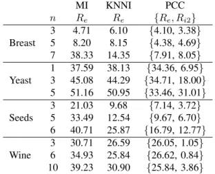
We use the four real data sets (Breast cancer, Seeds, Yeast and Wine data sets) available from UCI Machine Learning Repository to test the performance of PCC with respect to MI and KNNI. Three classes (CY T, N U C and M E3) are selected in Yeast data set to the evaluate our method, since these three classes are close and difficult to classify. The basic information of the four data sets is given in Table I, and the detailed information can be found at http://archive.ics.uci.edu/ ml/.
The k -fold cross validation was performed on the four data sets by the different classification methods, and k generally remains a free parameter. We used the simplest 2-fold cross validation7 here, since it has the advantage that the training and test sets are both large, and each sample is used for both training and testing on each fold. Each test sample has n missing (unknown) values, and they are missing completely at random in every dimension. The average error rate Rea
and imprecision rate Ria (for PCC) of the different classical
methods with values ofK ranging from 5 to 20 are given in Table II.
The results of Table II clearly show that the PCC method produces lower error rate than the MI and KNNI classification methods, but meanwhile it yields some imprecision in the classification result due to the introduction of meta-classes
7More precisely, the samples in each class are randomly assigned to two
sets S1and S2having equal size. Then we train on S1 and test on S2, and
reciprocally.
Table I
BASIC INFORMATION OF THE USED DATA SETS.
name classes attributes instances Breast 2 9 699 Seeds 3 7 210 Wine 3 13 178 Yeast 3 8 1050
Table II
CLASSIFICATION RESULTS FOR DIFFERENT REAL DATA SETS(IN%).
MI KNNI PCC n Re Re {Re, Ri2} 3 4.71 6.10 {4.10, 3.38} Breast 5 8.20 8.15 {4.38, 4.69} 7 38.33 14.35 {7.91, 8.05} 1 37.59 38.13 {34.36, 6.95} Yeast 3 45.08 44.29 {34.71, 18.00} 5 51.16 50.95 {33.46, 31.01} 3 21.03 9.68 {7.14, 3.72} Seeds 5 33.49 12.54 {9.67, 6.70} 6 40.71 25.87 {16.79, 12.77} 3 30.71 26.59 {26.05, 1.05} Wine 6 34.93 25.84 {26.62, 0.84} 10 39.23 30.90 {25.84, 3.86}
to reflect that some incomplete objects are very difficult to classify because of lack of discriminant information. The increasing of the number (i.e. n) of missing values in each test sample generally causes the increment of error rate in the three classifiers. The imprecision rate becomes bigger in PCC, since the more missing values lead to the bigger imprecision (uncertainty) in the classification problem. So the credal classification including meta-class is very useful and efficient here to represent the imprecision degree and it can help also to decrease the misclassification rate. The PCC approach allows to indicate that the objects in meta-classes are really difficult to be correctly classified, and they should be cautiously treated in the applications. If one wants to get more precise results, some other (possibly costly) techniques seem necessary to discriminate and classify such uncertain objects.
V. CONCLUSION
A new prototype-based credal classification (PCC) method has been presented in this work for classifying incomplete patterns thanks to the belief function framework. This PCC method allows the object (incomplete pattern) to belong to specific classes and meta-class (i.e. union of several specific classes) with different masses of belief. The meta-class is used to characterize the imprecision of the classification due to the missing values and it can also reduce errors. Once the PCC result indicates that an incomplete pattern belongs to a meta-class, it means that the specific classes included in the meta-class are undistinguishable based on the known partial available attributes. This incomplete pattern with uncertain
classification should be treated more cautiously in the appli-cation. If one wants to get more precise result, some more (possibly costly) techniques or information sources must be developed and used. Several experiments with artificial and real data sets have been done to evaluate the performances of PCC with respect to classical MI and KNNI methods. Our results show that PCC is able to well represent the imprecision of classification caused by the missing data, and reduce the classification error rate.
Acknowledgements
This work has been partially supported by National Natural Science Foundation of China (Nos.61135001, 61374159) and the Fundamental Research Funds for the Central Universities (No. 3102014JCQ01067).
REFERENCES
[1] P. Garcia-Laencina, J. Sancho-Gomez, A. Figueiras-Vidal A, Pattern
classification with missing data: a review, Neural Comput Appl. Vol.19,
pp.263–282, 2010.
[2] R.J. Little, D.B. Rubin, Statistical Analysis with Missing Data, 2nd Edition, John Wiley & Sons, New York, 2002.
[3] Z. Ghahramani, M.I. Jordan, Supervised learning from incomplete data
via an EM approach, In: Cowan JD et al. (Eds) Adv. Neural Inf.
Process., Morgan Kaufmann Publishers Inc.), Vol. 6, pp.120–127, 1994. [4] K. Pelckmans, J.D. Brabanter, J.A.K. Suykens, B.D. Moor, Handling
missing values in support vector machine classifiers, Neural Networks,
Vol. 18, No. 5–6, pp. 684–692, 2005.
[5] A. Farhangfar, L. Kurgan, J. Dy, Impact of imputation of missing values
on classification error for discrete data, Pattern Recognition Vol. 41,
pp. 3692–3705, 2008.
[6] J.L. Schafer, Analysis of incomplete multivariate data, Chapman & Hall, Florida, 1997.
[7] G. Batista, M.C. Monard, A Study of K-Nearest Neighbour as an
Imputation Method, in Proc. of Second International Conference on
Hybrid Intelligent Systems (IOS Press, v. 87), pp. 251–260, 2002. [8] G. Shafer, A mathematical theory of evidence, Princeton Univ. Press,
1976.
[9] F. Smarandache, J. Dezert (Editors), Advances and applications of
DSmT for information fusion, American Research Press, Rehoboth, Vol.
1-3, 2004-2009.
[10] P. Smets, Analyzing the combination of conflicting belief functions, Information Fusion, Vol.8, No.4, pp. 387–412, 2007.
[11] A.L. Jousselme, C. Liu, D. Grenier, E. Boss´e, Measuring ambiguity in
the evidence theory, IEEE Trans. on SMC, Part A: 36(5), pp. 890–903,
Sept. 2006.
[12] H. Laanaya, A. Martin, D. Aboutajdine, A. Khenchaf, Support vector regression of membership functions and belief functions - Application
for pattern recognition, Information Fusion, Vol. 11, No.4, pp. 338–350,
2010.
[13] T. Denœux, A k-nearest neighbor classification rule based on
Dempster-Shafer Theory, IEEE Trans. on Systems, Man and Cybernetics, Vol.25,
No.5, pp. 804–813,1995.
[14] T. Denœux, A neural network classifier based on Dempster-Shafer
theory, IEEE Trans. on Systems, Man and Cybernetics A, Vol. 30,
No. 2, pp. 131–150, 2000.
[15] Z.g. Liu, Q. Pan, J. Dezert, A new belief-based K-nearest neighbor
classification method, Pattern Recognition, Vol. 46, No. 3, pp. 834–
844, 2013.
[16] T. Denœux, P. Smets, Classification using belief functions: relationship
between case-based and model-based approaches, IEEE Trans. on
Systems, Man and Cybernetics, Part B: Vol.36, No.6, pp. 1395–1406, 2006.
[17] M.H. Masson, T. Denœux, ECM: An evidential version of the fuzzy
c-means algorithm, Pattern Recognition, Vol.41,No.4, pp. 1384–1397,
2008.
[18] T. Denœux, M.H. Masson, EVCLUS: EVidential CLUStering of
prox-imity data, IEEE Trans. on Systems, Man and Cybernetics Part B,
Vol.34,No.1, pp. 95–109, 2004.
[19] Z.g. Liu, J. Dezert, G. Mercier, Q. Pan, Belief C-Means: An extension
of fuzzy c-means algorithm in belief functions framework, Pattern
Recognition Letters, Vol.33,No.3, pp. 291–300, 2012.
[20] Z.g. Liu, J. Dezert, Q. Pan, Y.m. Cheng, A new evidential c-means
clustering method, Proceedings of the 15th International Conference
on Information Fusion (FUSION 2012), Jul. 2012, Singapore. [21] Z.g. Liu, J. Dezert, Q. Pan, G. Mercier, Combination of sources of
evidence with different discounting factors based on a new dissimilarity
measure, Decision Support Systems, Vol. 52, pp. 133–141, 2011.
[22] T. Denœux, Maximum likelihood estimation from uncertain data in the
belief function framework, IEEE Transactions on Knowledge and Data
Engineering, Vol.25, No.1, pp. 119–130, 2013.
[23] A. Tchamova, J. Dezert, On the behavior of Dempster’s rule of
combi-nation and the foundations of Dempster-Shafer theory, in Proceedings
of IEEE 6th International Conference on Intelligent Systems (IS’12), Sofia, Bulgaria, September, 2012.
[24] J. Dezert, A. Tchamova, On the validity of Dempster’s fusion rule
and its interpretation as a generalization of Bayesian fusion rule, Int.
Journal of Intelligent Sysytems (Special Issue: Advances in Intelligent Systems), Vol. 29, No. 3, pp. 223–252, 2014.
[25] F. Smarandache, J. Dezert, On the consistency of PCR6 with the
averaging rule and its application to probability estimation, in Proc. of
Fusion 2013 Int. Conference on Information Fusion, Istanbul, Turkey, July 9-12, 2013.
[26] A. Tchamova, J. Dezert, On the Behavior of Dempster’s rule of
combination and the foundations of Dempster-Shafer theory(best paper
award), Proc. of 6th IEEE Int. Conf. on Intelligent Systems IS ’12, Sofia, Bulgaria, pp. 108–113, Sept. 2012.
[27] L.M. Zouhal, T. Denœux, An evidence-theoretic k-NN rule with
param-eter optimization, IEEE Trans. on Systems, Man and Cybernetics, Part