HAL Id: hal-00444661
https://hal.archives-ouvertes.fr/hal-00444661
Submitted on 16 Dec 2020
HAL is a multi-disciplinary open access
archive for the deposit and dissemination of
sci-entific research documents, whether they are
pub-lished or not. The documents may come from
teaching and research institutions in France or
abroad, or from public or private research centers.
L’archive ouverte pluridisciplinaire HAL, est
destinée au dépôt et à la diffusion de documents
scientifiques de niveau recherche, publiés ou non,
émanant des établissements d’enseignement et de
recherche français ou étrangers, des laboratoires
publics ou privés.
Siegel distance-based covariance matrix selection for
Space-Time Adaptive
Marc Oudin, Jean-Pierre Delmas, Frédéric Barbaresco
To cite this version:
Marc Oudin, Jean-Pierre Delmas, Frédéric Barbaresco. Siegel distance-based covariance matrix
se-lection for Space-Time Adaptive. RADAR 2009 : International Radar Conference ”Surveillance for a
safer world”, Oct 2009, Bordeaux, France. �hal-00444661�
Siegel distance-based covariance matrix selection
for Space-Time Adaptive Processing
M. Oudin
1, J.P. Delmas
2and F. Barbaresco
31
Thales Airborne Systems, 2 avenue Gay Lussac, 78851 Elancourt, France
phone:+(33).1.34.81.31.29
email: [email protected]
2
Institut TELECOM, Telecom ParisSud, D´epartement CITI, CNRS UMR-5157,
9 rue Charles Fourier, 91011 Evry, France
phone:+(33).1.60.76.46.32, fax:+(33).1.60.76.44.33
email: [email protected]
3
Thales Air Systems, Strategy Technology and Innovation Department,
Surface Radar Business Line, Hameau de Roussigny, 91470 Limours, France
phone:+(33).1.64.91.99.24
email: [email protected]
Abstract—This paper presents a new criterion to deal with
training data heterogeneity in space-time adaptive processing (STAP). It is based on Siegel measure, which is a distance in the space of Hermitian positive definite matrices, and consists in computing the distance between the covariance matrix estimated from training data and an a priori matrix. After deriving a test based on this distance, the statistical behavior of Siegel distance is analyzed, as a function of the number of training samples. Its probability density function (PDF) is derived and related to that of the generalized inner product (GIP) in the case of one single training snapshot. Finally, simulations are performed to illustrate the interest of preprocessing training data using Siegel distance, in terms of STAP signal to interference plus noise ratio (SINR) performance.
Index Terms—STAP, Siegel distance, Generalized Inner
Prod-uct
I. INTRODUCTION
STAP is a well-known technique used for clutter mitigation in radar applications among any others. For a cell under test (CUT), STAP algorithms are based on the estimation of the covariance matrix of clutter and background noise. In an ideal situation, there exist training samples which are independent and identically distributed (i.i.d.) and share the same covariance matrix. In that case, the true covariance ma-trix is estimated by its maximum-likelihood covariance mama-trix (the sample covariance matrix (SCM) under the assumption of Gaussian training samples) and the estimation improves when the number of training samples increases. Consequently, the performance of adaptive filters increases with the number of training samples. For instance, when the sample matrix inversion (SMI) STAP processor [1] is used, the average SINR performance becomes within 3 dB of the optimal performance when more than 2N (where N is the number of space-time degrees of freedom) samples are used.
However, in practical applications, i.i.d. training samples are scarce since the environments are very frequently hetero-geneous (e.g., see [2]). Since the presence of heterohetero-geneous samples (outliers) in the training data, leads to a biased covari-ance matrix estimate, the performcovari-ance of adaptive algorithms degrade. To take this problem into account, preprocessing schemes of the training data have been developed. An im-portant class of solutions are based on non homogeneity detection (NHD). The principle of NHD techniques is to detect and excise nonhomogeneous training snapshots to avoid a bias in the covariance matrix estimation and thus keep good SINR performance for STAP algorithms. For instance, the GIP [3], [4] is a commonly-used NHD technique which aims at detecting outliers in the training snapshots. For each sample x of the training data, it consists in computing a scalar value
equal to xHRb−1x, where bR is the SCM derived from all
the training data. Then, the resulting value is compared to a threshold and the sample is removed from the training samples if the value exceeds the threshold. Other techniques also exist, based for instance on power tests or on more sophisticated techniques like the projection statistics test (PS) [5].
In this paper, we consider the context of a forward-looking radar where data heterogeneity is mostly due to the pres-ence/absence of clutter in the training data and to the fact that clutter characteristics depend on physical parameters and vary with range and Doppler [6]. Other factors can also gen-erate heterogeneities such as for instance complex scattering environments. In that context, heterogeneous training data cannot only be modelled by discrete outliers, but other models must be developed [7]. In that condition, the use of NHD techniques may not be the most appropriate solution to deal with it. Moreover, although these techniques can be efficient to detect one or more outliers in the data, they can have an
high computational complexity since they need to process each of the different samples in the training data. The number of operations is therefore proportional to that number of training samples.
Here, we propose another approach which aims at having good SINR performance on powerful clutter areas, with-out degrading the performance with respect to conventional processing on other areas, and by minimizing the number of detection tests. It consists in computing a SCM with a few training samples in the neighborhood of the CUT (so that we limit clutter heterogeneity which extends with the distance to the CUT). Then, a test on the resulting SCM is performed to decide whether powerful clutter is present in the training data or not and whether there is a need to implement an adaptive filter or not. This test is significant since when a small number of samples are used to compute an adaptive filter, estimation errors occur, which limit the algorithm SINR performance. Choosing a non-adaptive filter on background noise therefore avoids those SINR performance losses. Then, let us note that compared to NHD techniques, this algorithm does not need any detection for each training sample, but only for the SCM computed for each CUT.
To test whether using a STAP filter based on the SCM is useful, we compute the distance between the background noise covariance matrix (which is assumed to be known in this paper) and the SCM. The chosen distance is the Siegel distance [8], which is defined on the space of Hermitian positive matrices.
This paper is organized as follows. In Section II, data model and problem statement are presented. Then, in Section III, the expression of Siegel distance is given and its PDF in the case of an SCM estimated with one training snapshot is derived. Finally, simulations are performed in Section IV to illustrate the SINR performance of the proposed scheme.
II. PROBLEM STATEMENT
A. Data model
Let us consider an airborne radar with an arbitrary array composed of N sensors. The radar emits an M -pulse wave-form. Then, let us suppose that the environment be composed of clutter, background noise and a moving target. For STAP processing, the data is divided into two sets of data called primary and secondary data. The primary data consists of the samples to be filtered and is composed of background noise, and possibly clutter and signal. The secondary data is the training data, and is supposed to be only composed of background noise and possibly clutter. We denote K the number of secondary samples used to compute adaptive filters and assume that for each adaptive filter, the K secondary samples used for its computation share the same distribution. The background noise is modelled by a zero-mean i.i.d. com-plex process not necessarily spatially white, with covariance matrix R. Then, the signal is considered as deterministic, with unknown power, but known direction and speed. Finally, the clutter is modelled by elementary reflectors. Those ones are supposed to be motionless, spatially and from pulse to pulse
correlated but white from sample to sample during a pulse. They are assumed to be zero-mean, with power depending on their direction of arrival (DOA) and distance.
B. Problem statement
STAP filtering consists in computing, for each sample of the primary data, an adaptive filter based on the inverse of
an estimated covariance matrix. Let us denote zi, the primary
sample to be filtered, Riits covariance matrix and zk(i)k=1..K
the secondary samples in the neighborhood of zi which are
used for the estimation of the covariance matrix Ri. This one
will be computed by: b Ri= 1 K K X k=1 zk(i)zk(i)H.
In the case where the secondary samples are composed of background noise alone Gaussian distributed, the estimated covariance will be distributed with the following Wishart distribution:
b
Ri∼ W(N, K, R).
Before filtering the primary sample, our problem is first to
decide whether bRi is the SCM of R (hypothesis H0) or
not. Then, to optimize the SINR, we apply the filter R−1φ
based on R under hypothesis H0 or the adaptive filter bR−1i φ
based on bRiotherwise, where φ is the spatio-temporal steering
vector of the target.
III. USE OFSIEGEL DISTANCE BETWEENHERMITIAN
POSITIVE DEFINITE MATRICES
A. Test based on Siegel distance
To test the hypothesis H0, we compute the distance between
b
Riand R. We choose the Siegel distance, since it is a distance
on the space of Hermitian positive definite matrices, with good invariance properties [9], [10]. This distance is defined by:
d(R, bRi)2 = ° ° °log(R−1/2RbiR−1/2) ° ° °2 = N X n=1 log2(λn)
where (λn)n=1...N are the generalized eigenvalues of ( bRi, R),
equal to the eigenvalues of R−1Rbi or R−1/2RbiR−1/2where
R−1/2 is an arbitrary square root of R. The test consists
in comparing d(R, bRi) with a threshold s. If the distance
is below the threshold s, we decide to implement processing using the a priori matrix R, whereas in the contrary case, we
implement STAP algorithm based on the SCM bRi. It is clear
that since R−1/2RbiR−1/2 ∼ W(N, K, I), under hypothesis
H0, where I is the identity matrix of dimension N , the test
based on this distance is constant false alarm rate (CFAR). Indeed, the joint density of the eigenvalues of R−1/2RbiR−1/2
and consequently that of d(R, .) only depends on K and N and not on the background covariance matrix.
B. Statistical analysis of Siegel distance
Now, to fix the threshold s, we need to analyze the statistical
behavior of Siegel distance.(A supprimer: First, we consider
the particular case K = 1). But deriving the theoretical PDF of the Siegel distance for arbitrary K is rather challenging except for the specific case K = 1. In this case, although d(R, .) is
not defined ( bRi is singular), the Siegel distance PDF can be
derived and compared to that of the GIP, using a regularization. For instance, let us add the known covariance matrice ²R and consider bRi+ ²R.
In that case, we have:
d(R, bRi+ ²R)2= N
X
n=1
log2(λn(R−1Rbi+ ²I)).
Since R−1Rbiis rank-one, it has a single non-zero eigenvalue
which is equal to
λ = Tr(R−1z1(i)z1(i)H)
= Tr(z1(i)HR−1z1(i))
= z1(i)HR−1z1(i)
which is equal to the GIP measure denoted Q. The largest
eigenvalue of R−1Rbi+²I is therefore equal to Q+², whereas
the other eigenvalues are equal to ². In that case, the Siegel distance is then a function of the GIP measure, given by:
d(R, bRi) =
p
log(Q + ²)2+ (N − 1)log(²)2. (1)
When the data are composed of background noise alone,
the PDF of zk(i) is known, and the corresponding PDF of
Q can be computed. For instance, when zk(i) are Gaussian
distributed, it is well known that the PDF of Q follows a Chi-Squared distribution with N degrees of freedom [4], given by:
fQ(q) = q N −1
Γ(N )e
−q 0 ≤ q < ∞ (2)
where Γ(N ) is the Euler-Gamma function. Therefore, the PDF of the Siegel distance given by (1) can be easily deduced after a straightforward change of variable. It is given by:
fD(d) = 1 Γ(N )[(e √ d2−a − ²)N −1e−e √ d2−a+√d2−a+² + (e−√d2−a
− ²)N −1e−e−√d2−a−√d2−a+²
]√ d
d2− a (3)
for d >√a where a = (N − 1)log(²)2, which reduces to
fD(d) = (e d− 1)(N −1) Γ(N ) e d+1−ed 0 ≤ d < ∞ for ² = 1.
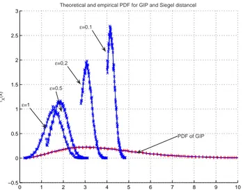
Fig.1 presents a comparison of the PDF of D obtained from Monte-Carlo realizations using simulated data with the theoretical value obtained by (3) for N = 4 with 4 values of ². In the simulation, we consider white noise, with unitary power, so that R = I. We note a goof fit between the theoretical and empirical PDF of the Siegel distance. Moreover, we observe that the mean of D tends to infinity whereas its variance
0 1 2 3 4 5 6 7 8 9 10 −0.5 0 0.5 1 1.5 2 2.5 3 x fX (x)
Theoretical and empirical PDF for GIP and Siegel distancel
ε=0.5
ε=0.2
ε=0.1
PDF of GIP
ε=1
Fig. 1. Theoretical (–) and empirical PDF for Siegel distance (××) and GIP (+ +).
converges to zero when ² tends to zero. That figure shows that the choice of ², which is arbitrary, defines different schemes associated with different thresholds s, each threshold being chosen to have a given type-I error, and therefore very dependent on the value of ². In the following, we will make the choice ² = 1 for simplicity. Then, for comparison, we also plot the empirical and theoretical PDF of Q obtained by (2). We note that whatever the value of ², the variance of Q is much larger than that of D which results from the application of the logarithm function in the definition of Siegel distance.
Then, we consider the case where K > 1. Since, ˆRi is not
positive definite for K < N , we still consider the regularized matrice. In that case, the derivation of the theoretical PDF of Siegel distance is challenging. Therefore, we only consider the
mean and variance of dK = d(R, ˆRi+ ²R) for K > 1. For
both moments, we compute asymptotic values w.r.t. K. We have: E{dK} = E{ v u u tXN n=1 log2(λn(R−1Rbi+ ²I))}
and E{d2K} is equal to
E{ v u u t XN n,n0=1
log2(λn(R−1Rbi+ ²I)) log2(λn0(R−1Rbi+ ²I))}.
For computing the limiting values of the mean and variance
of dK, when K → ∞, we use the continuity of the eigenvalue
function. Thus, we obtain
lim K→∞E{dK} = v u u tXN n=1 log2(λn((1 + ²)I)) = √N log(1 + ²)
0 0.5 1 1.5 2 2.5 3 0 0.5 1 1.5 2 2.5 x fX (x)
Empirical PDF of Siegel distance
K=1 K=2 K=4 K=16
K=1000
Fig. 2. Empirical (-+) PDF of Siegel distance for five values of K with
² = 1. and lim K→∞E{d 2 K} = v u u tXN n=1 N X n0=1
log2(λn((1 +²)I)) log2(λn0((1 +²)I))
= lim
K→∞E{dK}
2
which shows that the variance converges to zero when K increases to infinity1.
In Fig.2, we plot the empirical PDF for Siegel distance, for different values of K for N = 4, with ² = 1 and white noise
of unit power. We see that the variance of dK converges to
zero very rapidly. Then, in Tab.I, we compute the empirical
mean of dK as a function of K. We see that the asymptotic
value√N log(2) ≈ 1.386 is obtained very rapidly as well.
K 1 2 4 16 100 ∞
E{dK} 1.53 1.513 1.466 1.408 1.39 1.386
Tab.I: Empirical mean of dK as a function of K
IV. SIMULATIONS
We now illustrate the proposed scheme with simulations. Thus, let us consider the context of an airborne radar with rectangular array composed of N = 4 subarrays. More, precisely, we consider the case of a forward-looking radar, for which clutter is distributed along an ellipse in the angle-Doppler plane which varies with distance [6]. This naturally leads to clutter heterogeneity. Therefore, for each primary sample to filter, the number of secondary samples K sharing the same distribution as the CUT is limited. Consequently, errors occur in the estimation of the noise covariance matrix, what leads to performance degradation. In Fig.3, we illustrate clutter heterogeneities by showing a clutter + noise power map.
1Let us note that this is a natural result since bRiis a consistent estimate
of R.
Doppler cell number
Range cell number
Power map 50 100 150 200 250 10 20 30 40 50 60
Fig. 3. Power map vs range and Doppler cell.
The number of pulses is equal to M = 256 and the number of range cells is equal to 60. The objective of the proposed processing is to attain the maximal STAP SINR performance. In the illustrations, we plot the normalized SINR, i.e., the ratio between the SINR and its optimal value (obtained in exact statistics with background noise alone).
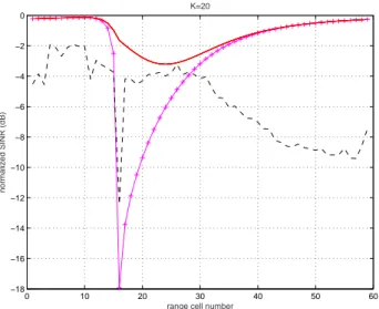
First, we compare in terms of SINR performance, the standard STAP processing based on the estimation of the noise covariance matrix, to the processing based on a priori background noise covariance matrix (that will be called in the following a priori processing), which is optimal with background noise alone. Thus, we plot in Fig.4 the normalized SINR for both STAP processing (computed with the SMI algorithm with diagonal loading) and a priori processing, at
a given (peut ˆetre pr´eciser cette Doppler cell pour pouvoir
mieux s’appuyer sur la Fig.3)Doppler cell and with a number of training samples equal to K = 20. Both SINR must be compared to the optimal SINR which is reached under assumption of a known clutter + noise covariance matrix. Depending on the range cell, 3 areas must be distinguished. From range cell 0 to range cell 15, we observe that a priori processing is sufficient to attain optimal performance, since at those range cells, clutter is less powerful than background noise as can be seen from Fig.3. By comparison, STAP with
K = 20 samples leads to poor SINR performance. From range
cell 15 to range cell 30, clutter is powerful and performance of a priori processing significantly degrades. In that case, STAP is very useful since it allows to increase the SINR up to about
10 dB.Note that at range cell 17, the clutter that is present in
the SCM estimated from the cells around it, is very strong (as shown by the power map in Fig.3), whereas it is not present in the a priori covariance matrix. Finally, the 3rd area is between range cell 30 to 60, where the performance of a priori processing becomes better than those of STAP, though clutter is more powerful than background noise, as shown by
0 10 20 30 40 50 60 −18 −16 −14 −12 −10 −8 −6 −4 −2 0
range cell number
normalized SINR (dB)
K=20
Fig. 4. Normalized SINR vs range cell, at Doppler cell 100, for optimal
(—), a priori (+-+) and STAP algorithm (- - -).
0 10 20 30 40 50 60 −18 −16 −14 −12 −10 −8 −6 −4 −2 0
range cell number
normalized SINR (dB)
K=20
Fig. 5. Normalized SINR vs range cell, at Doppler cell 100, for optimal
processing (–), and the proposed scheme (*).
power map in Fig.3.
Then, we implement the proposed scheme. Depending on the value of Siegel distance, it consists in choosing between a priori and estimated from training data covariance matrix, for space-time processing. In Fig.5, we compare the resulting normalized SINR of the proposed scheme to the optimal SINR. The threshold s is chosen by use of Monte Carlo simulations with background noise alone, so that the type-I error is less than 10−6.
We observe that this scheme makes a good choice between conventional STAP and a priori filter since it allows to attain good SINR performance. It allows both to improve the performance of conventional STAP processing on the areas of background noise alone (except in the close vicinity of clutter
discontinuities) and to avoid significant SINR losses, resulting from the presence of clutter, when using a priori processing. Finally, let us note that the use of this scheme can be extended to the case where several a priori matrices are available, for instance for knowledge-aided STAP.
V. CONCLUSIONS
In this paper, we have considered the use of Siegel distance, in radar array processing. We have proposed to compute the distance between the SCM of training data and an a priori covariance matrix before STAP processing, to decide what kind of filter to use. After having analyzed the statistical behavior of the Siegel distance, we have performed simulations to illustrate the interest of that preprocessing in terms of STAP SINR performance.
REFERENCES
[1] I. Reed, D. Mallet, L. Brennan, “Rapid convergence rate in adaptive arrays,” IEEE Trans. Aerosp. Electron. Syst.”, vol. 10, no. 6, pp. 853-863, Nov. 1974.
[2] W.L. Melvin, “Space-time adaptive radar performance in heterogeneous clutter,” IEEE Trans. Aerosp. Electron. Syst.”, vol. 36, no. 2, pp. 621-633, Apr. 2000.
[3] P. Chen, “Screening Among Multivariate Normal Data”, Journal of
Multivariate Analysis, 69, pp. 10-29, 1999.
[4] M. Rangaswamy, B. Himed, J.H. Michels, “Statistical Analysis of the Nonhomogeneity Detector”, Proc. Asilomar Conference on Signals,
Systems and Computers, vol. 2, pp. 1117-1121, Nov. 2000.
[5] G.N. Schoenig, M. L. Picciolo, “Improved Detection of Strong Nonho-mogeneities for STAP via Projection Statistics”, in Proc. of the IEEE
2005 International Radar Conference, Arlington, Virginia, 9-12, pp.
405-412, May 2005.
[6] R. Klemm, Principles of Space-Time Adaptive Processing, ser. IEE Radar, Sonar, Navigation and Avionics Series 12. London, U.K.: The Inst. Elec. Eng., 2002.
[7] S. Bidon, O. Besson, and J.Y. Tourneret, “A Bayesian approach to adaptive detection in non-homogeneous environments”, IEEE Trans.
Signal Process., vol. 56, no. 1, pp. 205-217, Jan. 2007.
[8] C.L. Siegel, Symplectic Geometry, Academic Press, New York, 1964.
[9] F. Barbaresco, “Innovative Tools for Radar Signal Processing Based on Cartan’s Geometry of SPD Matrices and Information Geometry”, in
Proc. of the IEEE International Radar Conference, Rome, May 2008.
[10] F. Barbaresco, ”Interactions between Symmetric Cones and Information Geometrics: Bruhat-Tits and Siegel Spaces Models for High Resolution Autoregressive Doppler Imagery”, ETCV’O8 Conference, Ecole Poly-technique, Nov. 2008, published by Springer.