HAL Id: hal-02118475
https://hal.archives-ouvertes.fr/hal-02118475
Submitted on 3 May 2019
HAL is a multi-disciplinary open access
archive for the deposit and dissemination of
sci-entific research documents, whether they are
pub-lished or not. The documents may come from
teaching and research institutions in France or
abroad, or from public or private research centers.
L’archive ouverte pluridisciplinaire HAL, est
destinée au dépôt et à la diffusion de documents
scientifiques de niveau recherche, publiés ou non,
émanant des établissements d’enseignement et de
recherche français ou étrangers, des laboratoires
publics ou privés.
of underwater mines in high resolution SAS images
Frederic Maussang, Jocelyn Chanussot, Michèle Rombaut, Maud Amate
To cite this version:
Frederic Maussang, Jocelyn Chanussot, Michèle Rombaut, Maud Amate. From statistical detection
to decision fusion : detection of underwater mines in high resolution SAS images. Advances in Sonar
Technology, edited by Sergio Rui Silva, In-Tech, pp.111 - 150, 2009, 978-3-902613-48-6. �hal-02118475�
From Statistical Detection to Decision Fusion:
Detection of Underwater Mines
in High Resolution SAS Images
Frédéric Maussang
1, Jocelyn Chanussot
2, Michèle Rombaut
2and Maud Amate
31
Institut TELECOM; TELECOM Bretagne; UeB; CNRS UMR 3192 Lab-STICC
2GIPSA-Lab (CNRS UMR 5216); Grenoble INP
3Groupe d’Etudes Sous-Marines de l’Atlantique DGA/DET/GESMA Brest
France
1. Introduction
Among all the applications proposed by sonar systems is underwater demining. Indeed, even if the problem is less exposed than the terrestrial equivalent, the presence of underwater mines in waters near the coast and particularly the harbours provoke accidents and victims in fishing and trade activities, even a long time after conflicts.
As for terrestrial demining (Milisavljevi et al., 2008), detection and classification of various types of underwater mines is currently a crucial strategic task (U.S. Department of the Navy, 2000). Over the past decade, synthetic aperture sonar (SAS) has been increasingly used in seabed imaging, providing high-resolution images (Hayes & Gough, 1999). However, as with any active coherent imaging system, the speckle constructs images with a strong granular aspect that can seriously handicap the interpretation of the data (Abbot & Thurstone, 1979). Many approaches have been proposed in underwater mine detection and classification using sonar images. Most of them use the characteristics of the shadows cast by the objects on the seabed (Mignotte et al., 1997). These methods fail in case of buried objects, since no shadow is cast. That is why this last case has been less studied. In such cases, the echoes (high-intensity reflection of the wave on the objects) are the only hint suggesting the presence of the objects. Their small size, even in SAS imaging, and the similarity of their amplitude with the background make the detection more complex.
Starting from a synthetic aperture image, a complete detection and classification process would be composed of three main parts as follows:
1. Pixel level: the decision consists in deciding whether a pixel belongs to an object or to the background.
2. Object level: the decision concerns the segmented object which is “real” or not: are these objects interesting (mines) or simple rocks, wastes? Shape parameters (size,…) and position information can be used to answer this question.
3. Classification of object: the decision concerns the type of object and its identification (type of mine).
This chapter deals with the first step of this process. The goal is to evaluate a confidence that a pixel belongs to a sought object or to the seabed. In the following, considering the object
characteristics (size, reflectivity), we will always assume that the detected objects are actual mines. However, only the second step of the process previously described, which is not addressed in the chapter, would give the final answer.
We propose in the chapter a detection method structured as a data fusion system. This type of architecture is a smart and adaptive structure: the addition or removal of parameters is easily taken into account, without any modification of the global structure. The inputs of the proposed system are the parameters extracted from an SAS image (statistical in our case). The outputs of the system are the areas detected as potentially including an object.
The first part of the chapter presents the main principal of the SAS imaging and its use for detection and classification. The second part is on the extraction of a first set of parameters from the images based on the two first order statistical properties and the use of a mean – standard deviation representation, which allow to segment the image (Maussang et al., IEEE, 2007). A third part enlarges this study to the higher order statistics (Maussang et al., EURASIP, 2007) and their interest in detection. Finally, the last part proposes a fusion process of the previous parameters allowing to separate the regions potentially containing mines (“object”) from the others (“non object”). This process uses the belief theory (Maussang
et al., 2008). In order to assess the performances of the proposed classification system, the results, obtained on real SAS data, are evaluated visually and compared to a manually labeled ground truth using a standard methodology (Receiver Operating Characteristic (ROC) curves).
2. SAS technology and underwater mines detection
SAS (Synthetic Aperture Sonar) history is closely linked to the radar one. Actually, the airborne radar imagery was the first to develop the process of synthetic aperture in the 1950’s (SAR : Synthetic Aperture Radar). Then, it was applied to satellite imagery. The first satellite to use synthetic aperture radar was launched in 1978. Civilian and military applications using this technique covered enlarged areas with an improved resolution cell. Such a success made the synthetic aperture technique essential to obtain high resolution images of the earth. Following this innovation, this technique is now frequently used in sonar imagery (Gough & Hayes, 2004). The first studies in synthetic aperture sonar occurred in the 1970’s with some patents (Gilmour, 1978, Walsh, 1969, Spiess & Anderson, 1983) and articles on SAS theory by Cutrona (Cutrona, 1975, 1977).
2.1 SAS principle
Synthetic aperture principle is presented on Fig. 1 and consists in the coherent integration of real aperture beam signals from successive pings along the trajectory. Thus, the synthetic aperture is longer than the real aperture. As the resolution cell is inversely proportional to the length of the aperture, longer the antenna, better the resolution. In practice, the synthetic aperture depends on the movements of the vehicle carrying the antenna. Movements like sway, roll, pitch or yaw are making the integration along the trajectory more difficult. The synthetic aperture resolution is that of the equivalent real aperture of length LERA, given
by the expression:
R ERA
2
(
N
1
)
VT
L
Fig. 1. SAS principle
where N is the number of pings integrated, V is the mean cross-range speed, T is the ping rate and LR is the real aperture length.
Hence, the cross-range resolution at range R is given by:
ERA S
L
R
!
"
(2.2)The maximum travel length (N-1)VT corresponds normally (but not necessarily) to the cross-range width of the insonification sector, equal to R /Ltr when the transmitter has a
uniform phase-linear aperture of length Ltrand operates in far field. For large N, the LERA
given by (2.1) equals approximately twice this width; hence, the resolution is independent of range and frequency, and is given by the expression:
2
tr SL
"
!
(2.3)Let us note that the cross-range resolution of the physical array !R = R /LR. The resolution
gain g of the synthetic aperture processing is defined by the expression:
R ERA S R
L
L
g
"
"
!
!
(2.4) 2.2 SAS challengesNowadays, SAS is a mature technology used in operational systems (MAST’08). However, some challenges remain to enhance SAS performances. For example, a precise knowledge of the motion of the antenna will permit to obtain a better motion compensation and better focused images. There are also some studies to improve beamforming algorithms, more adapted to SAS processing. Another challenge lies in the reduction of the sonar frequency. Knowing that sound absorption increases with the frequency in environments like sea water or sediment, a logical idea is to decrease imagery sonar frequency. Yet, resolution is inversely proportional to frequency and length of antenna. So for a reasonable size of array,
the resolution remains quite low, especially for underwater minewarfare. SAS processing can then be used to artificially increase the length of the antenna and improve the resolution One of the purposes is the detection of objects buried in the sediment. Both civilian (pipeline detection, wreck inspection) and military (buried mines detection) applications are interested in this concept. GESMA conducted numerous sea experiments on SAS subject since the end of the 1990’s. Firstly, in 1999, in cooperation with the British agency DERA, high frequency SAS was mounted on a rail in Brest area (Hétet, 2000). The central frequency was 150 kHz, the frequency band was 60 kHz and the resolution obtained was 4 cm. Fig. 2 presents two images resulting from this experiment.
Fig. 2. On the left, SAS image and picture of the associated modern mine. On the right, SAS image and picture of the associated modern mines
Then, GESMA decided to work on buried mines and conducted an experiment with a low frequency SAS mounted on a rail in 1999. It was in Brest area, the sonar frequency was between 14 and 20 kHz (Hétet, 2003). Fig. 3 presents results of this experiment. We notice the presence of a large echo coming from the cylinder.
Fig. 3. SAS image of buried and proud objects at 20 m. C1 : buried cylinder ; R1 : buried rock ; S1 : buried sphere ; S2 : proud sphere
Fig. 3 shows that low frequencies allow to penetrate the sediment and to detect buried objects. Moreover, echoes are more contrasted on this image and there is a lack of the
shadows for the objects, making the classification more difficult. To go a step further, in 2002, a low frequency SAS was hull mounted onboard a minehunter (Hétet et al., 2004). Frequency was chosen between 15 and 25 kHz and Fig. 4 presents results of these trials conducted in cooperation with the Dutch agency TNO, Defence, Security and Safety.
Fig. 4. Low frequency SAS images. On the left, SAS image of three cylinders.
Downwards : proud cylinder, half buried cylinder, buried cylinder. In the middle : pictures of the supporting ship, the sonar and the three cylinders. On the right, SAS images of two wrecks in the bay of Brest.
Considering previous figures, low frequency and high frequency SAS images present an important difference. High frequency images allow detecting and classifying underwater objects thanks to their shadow when low frequency images present no more shadow but strong echoes. The idea is thus to use specificities of low frequency SAS to define a new approach to detect and classify buried objects.
3. Underwater mines detection using local statistical parameters
The key issue when designing a classification algorithm is to choose the right parameters discriminating the classes of interest. The two main approaches are (i) use of statistical knowledge about the process, (ii) use of expert knowledge, eventually derived from a physical model of the process. In this application, the statistical characteristics of the seabed pixels are well known and follow statistical laws (Rayleigh and Weibull distributions for instance). As a consequence, the data fusion process is based on the comparison of the statistical characteristics locally extracted for each pixel and these laws.
3.1 Statistical description of the SAS images
The sonar images, as any image formed by a coherent system (radar imagery is another example), are seriously corrupted by the speckle effect. They thus have a strong granular aspect. This noise comes from the presence of a large number of elements (sand, rocks, etc.) that are smaller than the wavelength and randomly distributed over the seabed. The sensor receives the result of the interference of all the waves reflected by these small scatterers within a resolution cell (Goodmann, 1976).
3.1.1 Speckle noise and the Rayleigh law
Sonar images provided by the sonar system are constructed by the speckle. This bottom reverberation comes from the presence of a large number of elements (sand, gravel, etc.) that are smaller than the wavelength of the used monochromatic and coherent illumination source. These elements are assumed to be randomly distributed on the seabed. As a consequence, the sensor records the result of the constructive and destructive interferences of all the waves reflected by these elementary scatterers contained in a resolution cell (Collet
et al., 1998, Schmitt et al., 1996).
The response of a resolution cell can thus be described by the following:
! " ! ! ! d N i i i j A j X jY a 1 . ) exp( ) exp(
$
#
%
(3.1)with A being the amplitude of the response on a resolution cell and
#
representing the phase. The phases are usually considered as independent and uniformly distributed over[
'
&
,
"
&
]
. With these assumptions, and if the number of elementary scatterers Ndwithin the resolution cell is large enough, the central limit theorem applies: X and Y can be considered as Gaussian random values. Consequently, the probability density function of amplitude A! X2"Y2 follows a Rayleigh distribution:
0 , 2 exp ) ( 2 2 2 )) ( * + , , -. ' ! A A A A p A R
/
/
(3.2)with / being the Rayleigh’s law specific parameter. This parameter is bound with the average intensity of the reflected waves.
The th-order moment of A is given by the following:
) * + , -. " 0 ! 2 1 ) 2 ( 2 /2 ) (
1
/
2
1 1 A (3.3)with ! being the Gamma function (
3
"4 ' ! ! " 0 0 ! ) 1
(z z e ttzdt). This results in an interesting property of the Rayleigh law: the standard deviation A and the mean !Aof the amplitude A
are linked by a simple proportionality relation:
A R A k
5
2
!! with 1.91 4' 6 !&
&
R k (3.4)This property leads to modeling the speckle as a multiplicative noise. As a matter of fact, the variation of amplitude induced by the speckle and characterized by parameter A is bound
by the mean amplitude (!A) with a multiplicative coefficient kR.
3.1.2 Non-Rayleigh models
The previous description of the speckle is the most usual and the most popular one. However, it is not satisfactory when the number of scatterers within a resolution cell (noted
Nd in the previous paragraph) significantly decreases. The central limit theorem does not
hold and the Rayleigh approximation is no longer valid. This case is frequently observed in high-resolution images (Collet et al., 1998, Mignotte et al., 1999) such as SAS images. In this case, the amplitude A is better described by a Weibull law:
0 , exp ) ( 1 ! ! " # $ $ % & '' ( ) ** + , -'' ( ) ** + , . -A A A A p A W / /
0
0
0
/
(3.5) with being the scale parameter and ! representing the shape parameter, strictly positive. These two parameters provide an increased flexibility compared to the Rayleigh law. Note that this law is a simple generalization of the Rayleigh distribution (in the special case1
0
. 2 and ! = 2, the Weibull law turns to a simple Rayleigh law). For a Weibull distribution, the th-order moment of A is given by:' ( ) * + , 2 3 .
/
4
0
5
4 4) 1 ( A (3.6)Therefore, the proportionality between and still holds, but with a coefficient kW(! ) function
of !: 2 ) / 1 1 ( ) / 2 1 ( ) / 1 1 ( ) (
/
/
/
/
2 3 -2 3 2 3 . W k (3.7)Note that for ! = 2, corresponding to the Rayleigh law, we obtain the same coefficient as in (3.4).
Other more complex non-Rayleigh approaches have been proposed in the literature to statistically describe the bottom reverberation in high-resolution sonar imaging. One of the most famous models is the K-distribution. For this model, the number of scatterers in a resolution cell Nd is supposed to be a random variable following a negative binomial
distribution. The amplitude A is then described by a law (called generalized K-distribution), a three parameters distribution function given by (Gu & Abraham, 2001):
0 , 2 ) ( ) ( 4 ) ( 0 1 1 1 0 1 0 1 0 1 0 1 0 ' ' ( ) * * + , ' ' ( ) * * + , 3 3 . -2 A A K A A p A K
5
4
4
5
4
4
5
4
4
4
4
4 4 4 4 (3.8) where "1 is the shape parameter, µ is the scale parameter, and "0 is the parameter bound tothe number of raw data averaged to figure out the pixel reflectivity. K"1- "0 is the modified
Bessel function of the second kind and order "1 - "0. This distribution describes a rapidly
fluctuating Rayleigh component modulated by a slowly varying !² component. The th-order moment of A is then given by:
)
(
)
(
)
2
/
(
)
2
/
(
1 0 1 0 2 1 0 ) (4
4
4
4
4
4
4
4
5
5
4 43
3
2
3
2
3
''
(
)
**
+
,
.
A (3.9)The relationship between A and !A is preserved, with a coefficient depending on the two parameters "1and "0: 2 1 2 0 2 1 2 0 1 0 1 0 1 0
)
2
/
1
(
)
2
/
1
(
)
(
)
(
)
2
/
1
(
)
2
/
1
(
)
,
(
!
!
"
!
!
!
!
#
$
$
$
$
$
$
$
$
$
$
Kk
(3.10)A Rayleigh mixture has been also proposed to describe SAS data, each scattering material within a resolution cell being characterized by one specific Rayleigh distribution (Hanssen et
al., 2003).
3.1.3 Application to experimental data
In this section, the performances of the different statistical models are compared using the SAS data presented in section 2 (Fig. 2). For this purpose, two tests are considered: the ² criterion and the Kolmogorov distance (Mignotte et al., 1999). The ² criterion d ² is estimated
according to the following relation (Saporta, 1990):
%
&
'
#"
#
r i i i inP
nP
k
d
1 2 2 ( (3.11)where ki is the number of realizations (number of pixels having the value i), Piis the
estimated probability of value i, r is the number of possible values, and n is the number of observations (in our case, the number of pixels).
With k’i being the number of realizations from 1 to i and p’i being the value for i of the
cumulative distribution function associated with pi, the Kolmogorov distance is defined as:
i i r i K
k
n
p
d
#
)
"
)
# ...1max
(3.12)The parameters of the Rayleigh and the Weibull laws are evaluated on the SAS image using a maximum-likelihood (ML) estimator. The estimated parameter
*ˆ
MLof the Rayleigh law(3.2) is given by the following (Schmitt et al., 1996):
'
##
n i i MLy
n
1 2 22
1
ˆ
*
(3.13)where n is the number of pixels and yiis the amplitude of pixel i.
Parameters and ! of the Weibull law (3.5) are estimated by
ˆ
MLand!ˆ
ML, respectively,given by the following (Mignotte et al., 1999):
k k ML
!
!
"# $ % lim ˆ (3.14) ML ML n i i ML y n ! ! ˆ / 1 1 ˆ 1 ˆ & & ' ( ) ) * + %,
% (3.15)with k = F( k-1), 0 = 1 (exponential law), and
!
"
"
"
"
# # # # $ # n i x i n i i n i i x i n i x i y y y y n y n x F 1 1 1 1 ln ln ) ( (3.16)These estimators are unbiased, consistent, and efficient (Collet et al., 1998).
The estimation of the K-law parameters is more problematic. Actually, there is no analytic expression for the derivative of a modified second kind Bessel function. Consequently, no ML estimation can be performed without approximations (Joughin et al., 1993). A moment’s method can then be used (3.9), even though it does not offer a closed-form solution.
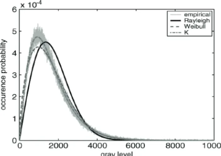
These estimators are tested on the image presented in section 2 (Fig. 2 left). Fig. 5 presents in solid line the observed distribution (normalized histogram of the image) and compares it with the estimated Rayleigh and Weibull distributions (dashed lines).With a simple visual inspection, one immediately notices that the Weibull distribution and K-distribution fit the observed one better than the Rayleigh distribution1. This confirms the nonvalidity of the
central limit theorem in the case of high-resolution images obtained in SAS imaging. This Rayleigh model will not be used subsequently. It is nevertheless included in this chapter
Fig. 5. Rayleigh distribution, Weibull distribution, and K-distribution estimated on Fig. 2
1 In Fig. 2 a shadow can be seen behind the echoes reflected by the mine. Shadows are
present on most sonar images containing underwater mines lying on the seabed. The shadow corresponds to a non illuminated region of the seabed and the sensor receives a weak acoustic wave from this region: the signal related to the shadow area essentially consists of the electronic noise from the processing chain. It can also come from the “differential shadow effect” due to the variation of the shadow zone position during the imaging process. The amplitude A of the pixels in this region can thus also be modeled by a Gaussian distribution and the models remain valid.
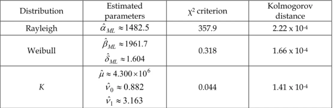
since the reader dealing with low-resolution sonar images may use the very same detection method proposed in this paper using the Rayleigh distribution. The K-distribution seems to provide a better statistical model of the background than the Weibull law. It especially fits better the “head” of the observed distribution. This is confirmed by the quantitative evaluation presented in Table 1. However, the “tail” of the distribution is accurately estimated by both models.
Distribution Estimated parameters 2 criterion Kolmogorov distance Rayleigh
!
ˆML 1482.5 357.9 2.22 x 10⁻⁴ Weibull 1961.7 ˆ ML " 604 . 1 ˆ ML # 0.318 1.66 x 10 -4 K 6 10 300 . 4 ˆ $ % 882 . 0 ˆ0&
163 . 3 ˆ1&
0.044 1.41 x 10⁻⁴Table 1. Comparison of the performances of the distribution on the SAS image of Fig. 2
3.1.4 Choice of the statistical model
Considering the previous remarks, the K-distribution seems to be a better model than the Weibull model. However, as we have seen in section 3.1.2, the estimation of K-law parameters is more difficult (no ML estimators). The estimators of the K-parameters are not optimal and the estimation takes more time.
The difference with the Weibull model is not enough to justify this difficulty. Moreover, Weibull law is largely used in the sonar community and it made its proofs in their applications. That is why we will use the Weibull model in the following, but we keep in mind the existence of other models such as K.
3.1.5 Local statistical description
In the previous sections, a global statistical description of the SAS images has been given, ignoring the presence of any echoes. This is fair since the number of target pixels in the image is too small to significantly modify the global statistics. The observed histogram matches indeed very well a Weibull law. In this section, we study local first- and second-order statistical properties. This is achieved by looking at the data through a small sliding window composed of few pixels. In this case, the potential presence of echoes can no longer be ignored. Each echo is modeled as a deterministic element with an amplitude D surrounded by a noisy background with a Weibull distribution. We assume that the noise correlation is smaller than the spatial extension of the target echo and that the amplitude fluctuation of the echo is negligible. This is consistent with the experiments where the echoes appear as small sets of connected pixels with an almost constant value. This is justified in Fig. 8(b) with the pixels corresponding to echoes fitting the predicted ellipse in the mean–standard deviation plane.
We note p the proportion of deterministic pixels (i.e., pixels belonging to an echo) and (1 – p) the proportion of random values (i.e., pixels belonging to the background) within a small square window (Fig. 6). Considering ’D(r), ’N(r), and ’W(r) , the rth-order noncentral
moments computed on the “echo part” of the window, the “background part” of the window, and the whole window, respectively, the following relation holds:
) ( ) ( ) (r Dr (1 ) Nr W! $ p ! # "p ! (3.17)
Considering X = ’X(1)and ²X = ’X(2) - ’²X(1), the mean and the variance of X, respectively
[X can be replaced by D, N, or W, as in (3.17)], we have:
N
W $p D#( "1 p) (3.18)
%
2 2&
%
&
%
2 2&
22 1 W N N D D W p
'
p'
'
$ # # " # " (3.19)Moreover, echoes are considered as deterministic elements with an amplitude D, leading to:
r r D
$
D
!
( ) (3.20) and D$D and'
D $0 (3.21) and, consequently: W $ N# p%
D" N&
(3.22)%
2 2 2&
2 2 2 2 N N W N N W'
pD'
'
$ # " # " " (3.23)By combining (3.22) and (3.23), we obtain an interesting relationship between W and W:
%
D
N&
W%
N&
D
W W(
N(
N'
2#
2$
#
"
'#
'"
(3.24) with(
'N$
'
N/
%
D
"
N&
2. It is important to underline that this relation is independent of p. Also note that in limit cases, this relation remains valid: in the case of p = 0 (the window contains only background pixels), W = N and !W = !N ; in the case of p = 1 (the echo is
filling the whole window), W = D and !W = 0, which is consistent with (3.21). Remember
that intermediate values of p correspond to windows being partially composed of echo pixels.
3.2 First and second order parameters: segmentation
The proportional relation of the statistical model describing the sea bed sonar data previously described is used to extract the two first parameters. The local mean and standard deviation are estimated on the SAS image using a square sliding window. These values become the coordinates of the processed pixel in the mean – standard deviation plane.
3.2.1 Mean-standard deviation representation
Inspired by a segmentation tool applied to spectrograms (Hory et al., 2002), this enables the separation of the echoes from the bottom reverberation, both features having different statistical characteristics as stated in section 3.1. In (Ginolhac et al., 2005), the link between first- and second-order statistics is highlighted using this representation.
Fig. 6. Modeled echo and various values of the parameter p: (a) p = 0, (b) p = 1/9, (c) p = 2/9, and (d) p = 1
Fig. 7. Building of the mean–standard deviation representation
Whereas in (Ginolhac et al., 2005) this link is simply illustrated as a justification to use first- and second-order statistics, the method presented in this chapter actually performs a segmentation of the mean–standard deviation plane.
The idea is to change the representation space of the data to highlight local statistical properties. The chosen space is the mean–standard deviation plane. For each pixel, the local standard deviation and the local mean are estimated within a square-centered computation window with the following conventional equations:
!
!
N i i Wy
N
11
ˆ
"
(3.25)#
$
!%
!
N i W i Wy
N
1 2ˆ
1
ˆ
"
&
(3.26)where N is the number of pixels in the computation window ( N = Nx.Ny with Nx and Ny
being the length and the width of the window, respectively) and yi is the value of pixel in
the window. The pair
#
ˆ
W,
"
ˆ
W!
becomes the coordinates representing the current pixel inthe mean–standard deviation plane (Fig. 7). The performances of these estimators are evaluated by computing their moments (Hory et al., 2002). For the mean estimator, the mean
!
W
M
"ˆ
and the varianceV
"ˆ
W!
are:!
W WM
"
ˆ
$
"
(3.27)!
N V W W 2 ˆ#
"
$ (3.28)The mean estimator is unbiased and consistent with a variance varying as 1/N. For the standard deviation estimator, the mean M
#
ˆW!
and the variance V#
ˆW!
are given by:!
!
!
W W W Wm
N
N
N
N
M
#
#
#
(4) 4 21
3
3
4
2
1
ˆ
%
%
%
%
&
(3.29)!
!
2!
4 ) 4 ( 23
1
4
1
ˆ
W W W WN
m
N
N
V
#
#
#
%
%
%
$
(3.30)with mW(4) being the fourth central moment computed on the window. These equations come
from the approximation
V
!
X
&
V
!
X
4
M
!
X
with X being a random variable (Kendall & Stuart, 1963). This estimator is asymptotically unbiased and is consistent with a variance varying as 1/N.The choice of the size of the computation window is a tradeoff. On one hand, the variance of the estimators [see (3.25) and (3.26)] increases for small values of N. N should thus not be too small to enable an accurate estimation. On the other hand, if N is too high, echoes being small elements, the proportion p of the deterministic elements in the computation windows remains low and echoes are lost in the background speckle [see (3.24)]. Consequently, the computation window should be chosen as slightly larger than the spatial extension of the echoes, this size depending on the resolution of the sonar image and the quality of the preprocessing chain.
The mean–standard deviation representation of Fig. 2 image is built with a 5 x 5-cm² window and is presented in Fig. 9. A general linear orientation is observed, as well as some pixels distancing the main direction on the right [see Fig. 8(b)]. Three different linear regressions of the data in the mean–standard deviation plane can be computed. They are shown in Fig. 8(a). The first line, with a slope of approximately 1.91, corresponds to the proportionality relation between the mean and the standard deviation estimated when assuming that the bottom reverberation is modeled by a Rayleigh law (3.4). The second line, with a slope of approximately 1.57, corresponds to the proportionality relation estimated with a Weibull model (3.7). At the given computation accuracy, the same line is obtained by a linear regression using a mean square method on the pixels representatives. To describe the global linear orientation of the data in the mean–standard deviation plane, the
proportionality coefficient estimated with the Weibull assumption clearly outperforms the estimation based on a Rayleigh law. This confirms the previous results for the case of high-resolution data (Table I). In Fig. 8(b), the curve corresponding to the local relationship between mean–standard deviation on a computation window (3.24) is plotted considering a deterministic element with an amplitude of D = 3.4 × 10⁻⁴, approximately corresponding to
the typical amplitude of the main echo on the original SAS image. This curve is a part of an ellipse and is a fairly good estimation of the main structure. Results obtained on other data sets could not be presented in this paper for confidentiality reasons. We will see following that each structure can be associated with one echo on the SAS image.
(a) (b)
Fig. 8. Mean–standard deviation representation of the SAS image (5 cm x 5-cm window). The linear approximations are estimated by the Rayleigh law, the Weibull law, and a regression. (a) Linear approximations. (b) Echo model
(a) (b)
Fig. 9. Comparison between the SAS image (Fig. 2) and its mean–standard deviation representation. (a) Zoom of the SAS image. (b) Representation
The fact that no pixel is on the Y-axis of this representation comes from the size of the computation window sensibly larger than the echoes. Therefore, no window contains only
echo pixels and all the windows have a part of background. Moreover, the hypothesis of a constant deterministic echo is not strictly valid, the pixels of one echo having different, but similar, values. However, the value of our model is not called into question to explain the results described previously.
To highlight interesting properties of the mean–standard deviation representation, it is compared with the original image. Fig. 9 presents a zoom of the original image featuring two mine echoes and the corresponding mean–standard deviation representation. For a better understanding, a manual labeling of the sonar image is performed: pixels corresponding to the echoes are selected and corresponding points on the mean–standard deviation representation can be inspected. It turns out that the cluster of points close to the origin of the mean–standard deviation plane corresponds to the bottom reverberation pixels on the SAS image, with low means and low standard deviations. On the contrary, horn-shaped structures (actually parts of ellipses) correspond to the echoes on the sonar image. Two main structures can be seen with different positions and dimensions, each one corresponding to one specific echo. The extremities of these structures correspond to the centers of the echoes which are deterministic elements (high mean and relatively low standard deviation). The intermediary points correspond to the transition between echoes and background (increasing standard deviation and decreasing mean). These properties can be used to classify the different elements on the sonar image by observing the mean– standard deviation plane and the characteristics of the different structures.
3.2.2 Segmentation
Based on the statistical study and the observations previously presented, we propose in this section a segmentation method. The aim is to design an automatic algorithm isolating the echoes from the reverberation background on the sonar images. The proposed method is decomposed into the following steps.
The Weibull distribution best fitting the observed normalized histogram is estimated with an ML estimator;
The original amplitude data are mapped in the mean–standard deviation plane; In this representation, echoes appear as horn-shaped structures whereas background
pixels are closer to the origin (low mean and low standard deviation). Therefore, a double threshold (both in mean and in standard deviation) allows a separation of the echoes pixels from the background pixels. The threshold value in standard deviation is set, either manually or automatically as will be described following;
Corresponding threshold value for the mean is obtained by multiplying the standard deviation threshold by the proportionality coefficient estimated for the Weibull law [see (3.7)];
Application of both thresholds in the mean–standard deviation plane isolates corresponding echoes pixels in the original image.
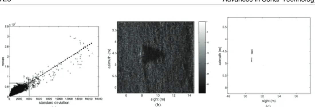
Fig. 10(b) presents an original sonar image. Corresponding mean–standard deviation representation is presented in Fig. 10(a) where the dashed line represents the proportionality coefficient between mean and standard deviation (estimated with the Weibull law), and the solid lines feature the threshold values. Corresponding segmentation of the image is presented in Fig. 10(c): the echoes have been correctly set apart.
To automate the segmentation algorithm proposed, we now propose a method to automatically set the standard deviation threshold value (the threshold value for the mean
Fig. 10. Segmentation of the SAS image of Fig. 2 (thresholds: standard deviation: 4000; mean: 6751). (a) Thresholds (in thick lines). (b) SAS image. (c) Result of the segmentation
is then set accordingly). This is achieved in stepwise fashion by means of a progressive segmentation: the results obtained with decreasing standard deviation thresholds are computed. For each result, the spatial distribution of the segmented pixels is studied by computing corresponding entropies2 with respect to the two axes, until a maximum value
was reached. For each result, the histograms of the segmented pixels along the X- and the Y-axis are computed and normalized (so that they sum to 1). See Fig. 12 for one example. Then, the entropy Haxis on each axis is computed by the following:
!
"
#$
%
I i axis axis axisp
i
p
i
H
log
2 (3.31)with paxis(i) being the number of segmented pixels (after normalization) in the column
(respectively, the line) number i, I = {I = 1…Naxis with paxis 0}, and Naxis being the number of
columns (respectively, lines) of the original image. These entropies characterize the spreading of the segmented pixels in the SAS image: a uniform distribution of the segmented pixels over the image leads to high entropies, whereas much localized regions lead to small entropies.
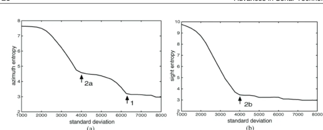
As a consequence, a decrease of the threshold value (more pixels are segmented) leads to an increase of the entropy (segmented pixels tend to distribute over the whole image). However, this increase is not regular (see Fig. 13): for instance, two slope break points clearly appear in the entropy evolution along the azimuth axis and one appears for the sight axis (they are pointed out by arrows in Fig. 13. They correspond to the standard deviation threshold of about 6250 and 4000, respectively). For a better understanding of these irregularities, the segmentations corresponding to different threshold values are presented in Fig. 11: when the threshold progressively decreases, the first echo begins to be segmented; then, the second echo is segmented as well which explains the rapid increase of the entropy (break point 1). Finally, the random background reverberation is reached, with segmented pixels spread all over the image. This explains the sharp increase of entropy (break point 2). Note that with the two segmented echoes being parallel to the azimuth axis, the first slope breaking is only visible on the azimuth axis (the sight axis only “sees” one echo).
2 Entropy-based segmentation algorithms have already been proposed in the literature. For
example, Pun used an entropy criterion, evaluated on the gray level histogram (Pun, 1980, 1981).
As a conclusion, the optimal segmentation, detecting both echoes with a maximal size but with no background element, is obtained with a threshold corresponding to the highest slope breaking (with a lower threshold, structures from the background are segmented generating false alarms in the system). This optimal threshold value is automatically detected from the derivative profile of the entropy. For this purpose, the maximum3 of the
two entropies defined previously is computed [see Fig. 14(a)]. The maximum of the derivative points out the highest slope breaking. However, to detect the real beginning of this slope breaking, the threshold corresponding to the half of this maximum is selected [see Fig. 14 (b)]. The result obtained on the SAS image from this threshold is presented in Fig. 12: the two echoes are correctly segmented.
Note that the computed threshold value is used in the following for the fusion process.
Fig. 11. Segmentation results for different thresholds in standard deviation. (a) Threshold 1000. (b) Threshold 5000. (c) Threshold 8000
Fig. 12. Segmented SAS image and repartition of the segmented pixels according to the two axes. Computed entropies: X-axis: 3.46; Y -axis: 4.58
3 Similar results are obtained with other combination operators (simple sum, quadratic sum,
Fig. 13. Entropy variation on the two axes in function of the threshold in standard deviation. (a) Azimuth axis. (b) Sight axis
Fig. 14. Maximum of the entropies, its derivative, and setting of the threshold (see the arrows). (a) Entropy (max). (b) Derivate entropy
3.3 Higher order statistics
Pertinent information regarding SAS data can also be extracted from higher-order statistics (HOSs). In particular, the relevance of the third-order (skewness) and the fourth order (kurtosis) statistical moments for the detection of statistically abnormal pixels in a noisy background is discussed in (Maussang et al., EURASIP, 2007). In this previous work, an algorithm aiming at detecting echoes in SAS images using HOS is described. It basically consists in locally estimating the HOS on a square sliding window.
3.3.1 HOS estimators
The two most classically used HOSs are the skewness (derived from the 3rd-order moment) and the kurtosis (derived from the 4th-order moment) (Kendall & Stuart, 1963). One should underline that beyond these two standard statistics, other statistics with an order greater than 4 can be mathematically defined. However, these statistics are extremely difficult to estimate in a reliable and robust way and are thus practically never used. Noting X(r) as the rth order central moment of a random variable X, the definition
2 / 3 ) 2 ( ) 3 ( X X X
S
!
(3.32)A definition of the kurtosis is given by:
3
2 ) 2 ( ) 4 ('"
!
X X XK
(3.33)The skewness measures the symmetry of a random distribution, while the kurtosis measures whether the data distribution is peaked or flat relative to a normal distribution. These statistics are theoretically zero for the normal distribution.
To estimate the skewness and the kurtosis on a sample X of finite size N, k-statistics kX(r) can
be used. kr is defined as the unique symmetric unbiased estimator of the cumulant X(r)on X
(Kendall & Stuart, 1963). An unbiased estimator of the skewness is then given by:
2 / 3 ) 2 ( ) 3 (
ˆ
X X XS
!
(3.34)Defining the rth sample central moment of X by the following expression:
"
#
$
!%
!
N i r i r Xx
x
N
m
1 ) (1
(3.35) where"
#
$
! ! N i xi N x 1 /1 and xi are the N samples of X, we can derive another definition of
this estimator. Actually, considering the relationships between kX(r) and mX(r), we have:
2 / 3 ) 2 ( ) 3 ( 2 ) 1 ( ˆ X X X m m N N N S % % ! (3.36)
In the same way, we derive the following estimator for the kurtosis:
) 3 )( 2 ( ) 1 ( 3 ) 3 )( 2 ( ) 1 )( 1 ( ˆ 2 2 ) 2 ( ) 4 ( 2 ) 2 ( ) 4 ( % % % % % % % & ! ! N N N m m N N N N k k K X X X X X (3.37)
Asymptotic statistical properties are studied for high values of N. Firstly, we can mention that these estimators are biased in the first order and that they are correlated (the bias being dependent on higher-order moments). However, exact results can be derived in the Gaussian case. In this case, M and V being the mean and the variance respectively, we have:
" #
SˆX !0 M" #
KˆX !0 M" #
N
N
N
N
N
N
S
V
X6
)
3
)(
1
)(
2
(
)
1
(
6
ˆ
'
&
&
%
%
!
(3.38)!
N
N
N
N
N
N
N
K
V
X24
)
5
)(
3
)(
2
)(
3
(
)
1
(
24
ˆ
2"
#
#
$
$
$
%
In the general case, there is no analytical expression for unbiased estimators independently from the probability density function of the random value. However, one should note that in the case of a normal distribution, the estimators are unbiased. Nevertheless, variances of these estimators are relatively high and it is well known that a reliable estimation requires a large set of samples.
3.3.2 Application on sonar images
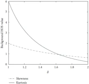
We have seen in section 3.1 that a good statistical model of the background noise in the case of high resolution sonar images is given by the Weibull law. With such a non-Gaussian distribution, background values of the skewness and the kurtosis are not null anymore. On real SAS data, [see (3.5)] is function of the resolution of the image, but it is generally approximated by 1.65 (Maussang et al., 2004). This corresponds to skewness and kurtosis values close to 1 (Fig. 15).
Fig. 15. Weibull background HOS values in function of the parameter of the Weibull law Considering the echoes generated by the mines as deterministic elements, the SNR is sufficiently high to have higher values of the HOS if the calculus window contains an echo (Maussang et al., EURASIP, 2007).
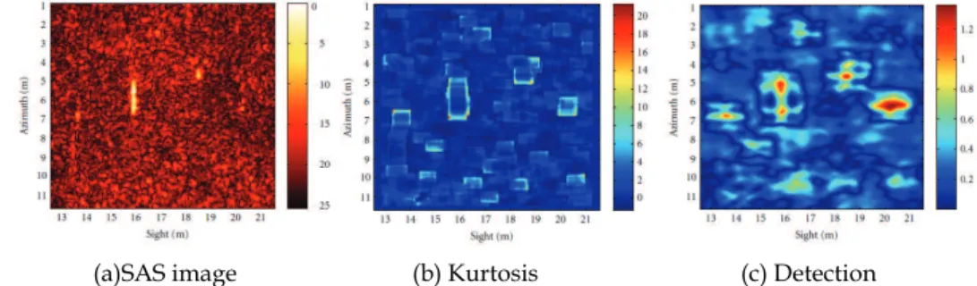
Fig. 16 presents the kurtosis results obtained on SAS image of Fig. 3 where all the objects of interests are framed by high values of the kurtosis, the size of the frame being linked to the size of the computation window. A theoretical model of these frames is used to perform a matched filtering and thus refocus the detection precisely at the center of the objects of interest. The last step consists in rebuilding the objects using a morphological dilation (Maussang et al., EURASIP, 2007). The corresponding detection result is presented in Fig. 16(c): all the objects of interest are marked by high values, thus providing a good detection.
However, some false alarms remain, and the detection is not as accurate as with the first algorithm (see section 3.2). This will be taken into account for the fusion process (section 4).
(a)SAS image (b) Kurtosis (c) Detection
Fig. 16. Detection on the SAS data of Fig. 3 (kurtosis 11 × 11, matched filtering 15 × 15, SD = 3).
4. Underwater mines detection using belief function theory
In the previous section, we have presented two algorithms aiming at detecting echoes in SAS images. In order to further improve the detection performances, we present a fusion scheme taking advantage of the different extracted parameters. The combination of parameters in a fusion process can be addressed using probabilities. This popular framework has a solid mathematical background (Duda & Hart, 1973). Numerous papers have been written on this theory using modeling tools (parametric laws with well-studied properties) and model learning. However, these methods are affected by some shortcomings. Firstly, they do not clearly differentiate doubt from conflict between sources of information. Single hypothesis being considered, the doubt between two hypotheses is not explicitly handled and the corresponding hypotheses are usually considered as equiprobable. Conflict is handled in the same way. Moreover, probabilities-based fusion methods usually need a learning step using a large amount of data, which is not necessarily available for an accurate estimation.
Another solution consists in working within the belief function theory (Shafer, 1976). The main advantage of this theory is the possibility to deal with subsets of hypotheses, called propositions, and not only with single hypothesis. It allows to easily model uncertainty, inaccuracy, and ignorance. It can also handle and estimate the conflict between different parameters. Regarding the problem of detection, this theory enables the combination of parameters with different scales and physical dimensions. Finally, the inclusion of doubt in the process is extremely valuable for the expert who can incorporate this information for the final decision. As a conclusion, the belief function theory is selected to address the considered application. The proposed fusion scheme is described in the next subsection.
4.1 Fusion scheme and definition of the mass functions
For the detection of echoes in SAS images, the frame of discernment defined for each pixel is composed of the two following hypotheses:
i. “object” (O) if the pixel belongs to an echo reflected by an object;
ii. “nonobject” (NO) if it belongs to the noisy background or a shadow cast on the seabed. The set of propositions 2 is thus composed of four elements: the two single hypothesis, also called singletons, O and NO, the set = {O,NO}, noted O U NO (U means logical OR) and
called “doubt,” and the empty set called “conflict.” In this application, the world is obvious closed ( contains all the possible hypotheses).
The proposed fusion process uses the local statistical parameters extracted from the SAS image, as presented in section 3. These parameters are fused as illustrated on Fig. 17: the relationship between the first two statistical orders is taken into account by using the thresholds in standard deviation and mean estimated by the automatic segmentation, the third and fourth statistical moments are used after focusing and rebuilding operations.
Fig. 17. Main structure of the proposed detection system
The mass of belief is the main tool of the belief function theory as the probability for the probability theory. The definition of the mass functions enables to model the knowledge provided by a source on the frame . In this application, every parameter is used as a source of information. For one given source i, a mass distribution mit on 2 is associated to each
value t of the parameter. This type of functions verifies the following property:
1 ) (
2
!
A# "m A . We propose to define each mass function by trapezes or semi trapezes.In the considered application, only the three propositions (O), (NO), and (O U NO) are concerned. Four thresholds must thus be defined namely, ti1, ti2, ti3, and ti4 (see Fig. 18). They
are set using knowledge on local and global statistics of sonar images. They also take into account the minimization of the conflicts while preserving the detection performances (no
nondetection).
The first mass function concerns the two first statistical orders simultaneously because they are linked by the proportional relationship. In order to build the trapezes, we consider the pair (mean; standard deviation) as used for the automatic segmentation. Fig. 19 illustrates the design of the corresponding mass function, based on the mean standard deviation representation. We first describe this function in the general case, the setting of the parameters being described afterward.
Pixels with a local standard deviation below t11 are assigned a mass equal to one for the
proposition “nonobject” and a mass equal to zero for the others. Pixels with a local standard deviation between t11 and t12 are assigned a decreasing mass (from one to zero) for the
meaning “object OR nonobject” (O U NO). These variations are linear in function of the standard deviation.
The construction of the mass functions goes in a similar way for t13 and t14. This mass
function is function of the standard deviation, but, considering the proportional relation holding between the mean and the standard deviation, an equivalent mass function can easily be designed for the mean. Then the mass function corresponding to the mean being redundant with the standard deviation is not computed.
We propose to set the different parameters of these mass functions using the following expressions:
!
B W M t1"
ˆ 1 # ;!
W B!
B WV
M
t
12#
"
ˆ
$
"
ˆ
;!
B W s V t"
"
ˆ 2 1 3 1 # % ; (4.1)!
B W s V t"
"
ˆ 2 1 4 1 # $where
"
ˆBstands for the background standard deviation estimated, using the Weibull modelpreviously computed, on a region of the image without any echo. s is the threshold in
standard deviation fixed by the algorithm described in section 3.2. MW and VW are the mean
and variance of the standard estimators (Kendall & Stuart, 1963) applied on s considering
the size of the computation window used for mean standard deviation building. This allows taking into account the uncertainty in the statistical parameters estimation by the fuzziness of the mass distributions.
Fig. 18. Definition of the mass functions
The two other mass functions concern the HOSs: the skewness and the kurtosis, respectively. As mentioned in section 3.3, the corresponding detector provides less accurate results, which prevent a precise definition of the areas of interest. Furthermore, some artifacts generate false alarms. As a consequence, the information provided by these parameters will only be considered to assess the certainty of belonging to the background. A null mass is thus systematically assigned to the proposition “object,” whatever are the values of the HOS. The mass is distributed over the two remaining propositions: “nonobject” and “doubt.” This is illustrated on Fig. 20: only two parameters remain t21 and t22.
Fig. 19. Definition of the mass functions for the first two-order statistical parameters:
!
WV
t
t
t
t
12$
11#
14$
13#
"ˆ
(the thresholds obtained from the automatic segmentation are in red. The mean standard deviation graph given on this figure has been calculated on the image presented on Fig. 4).Fig. 20. Definition of the mass functions for the higher-order statistics (the graphic is valid for definition of t31 and t32)
Parameters t21 and t22 (skewness) are set by considering the normalized cumulative
histogram, noted H(t), of the HOS values over the whole SAS image. This is illustrated in Fig. 21. Considering that pixels with low HOS values necessarily belong to the noisy background and that pixels with high values (that might belong to an echo of interest) are extremely rare, the following expressions are used:
!
75 . 0 1 1 2 $ #H t!
90 . 0 1 2 2 " # H t (4.2)These equations are valid for t31 and t32 (kurtosis). This assumes that at least 75% of the
image belongs to the background, which is easily fulfilled. Similarly, the 10% pixels with the highest HOS values are considered as potential objects (doubt has a mass equal to one).
Fig. 21. Example of histogram and cumulative histogram of a kurtosis image (after focusing and rebuilding, as presented on Fig. 16(c))
Based on the local statistical moments of the data, three mass functions have been defined. The data fusion aims at improving the detection performances and eases the final decision by the expert. It is performed using the following conjunctive rule:
3 2 1 3 , 2 , 1
m
m
m
m
#
$
$
(4.3)where $ is the conjunctive sum:
! !
( ) ( )2 1 2 1 m A m B m C m A C B
%
& # # $ with A a proposition.Note that, for the sake of simplicity, the superscript t of the mass mit, corresponding to the
parameter value, is removed from the notations.
A conflict between the different sources can appear during this combination phase. This information is preserved as it is valuable to assess the adequacy of the fused parameters. If one of the fused parameters provides irrelevant information, the conflict is high. Further investigations are then required to determine the cause of this situation (bad estimation of the parameter, limits of the data, etc.).
4.2 Decision
The results of the fusion step can be used in different ways, producing different end user products:
i. “binary” representations can be generated, providing segmented images and giving a clear division of the image into regions likely to contain objects or not;
ii. “enhanced” representations of the original SAS image can also be constructed from the results of the fusion.
These representations should somehow underline the regions of interest while smoothing the noise, but leave the decision to the human expert. The “binary” representations only use
the results of the fusion process in order to classify each pixel according to the belief, the plausibility, or the pignistic value. A simple solution consists in thresholding the belief or plausibility for the proposition “object,” for instance, all the pixels with a belief above 0.5 are assigned to the class “echo.” A binary image is obtained, separating the echoes from the background. However, this method requires the setting of the threshold by the user. In order to overcome this shortcoming, another strategy consists in associating each pixel to the hypothesis (“object” or “nonobject,” resp.) with the highest belief. This unsupervised method also provides a binary image. The same methods can be used with the plausibility. However, since the space of discernment only contains two elements, plausibility and belief actually provide the same results. The corresponding results are presented on different datasets on Fig. 22(d) and Fig. 23(d).
Beyond the binary result, a more precise classification can be constructed by assigning every pixel to the class with the highest mass of evidence (including the conflict). The resulting image is divided into four classes: “object,” “nonobject,” “doubt,” and “conflict.” Corresponding results are presented on Fig. 22(c) and Fig. 23(c). This nonbinary representation leaves more flexibility to the expert for the final interpretation. A similar strategy has been used in the frame of medical imaging in (Bloch, 1996).
Fig. 23. Presentation of the fusion results—image of Fig. 4
These representations are well suited for a “robotics oriented” detection: regions of interest are defined, and an automatic system, such as an autonomous underwater vehicle (AUV), can be sent to identify the objects. However, such representations lose a lot of potentially valuable information (environment, relief, intensity, etc.). Such information may be useful for a human expert to actually identify the objects and solve some ambiguities. Therefore,
other representations can be considered. For instance, we propose to combine the results of the fusion with the original image in order to enhance information. This is achieved by weighting the pixels of the original image by a factor linearly derived from the belief (or the plausibility) of the class “object.” The intensity of pixels likely NOT being echoes is decreased (low belief), thus enhancing the contrast with the pixels most likely being echoes. For instance, Fig. 22(b) and Fig. 23(b) feature the resulting images with the weighting factor linearly ranging from 0.3 for a null plausibility to 1 for a plausibility of 1. On these images, the background tends to disappear, but all potential objects of interest are preserved. Finally, another solution consists in performing an adaptive filtering of the sonar image in function of the belief. This is described in (Maussang et al., 2005).
4.3 Performance estimation
The decision coming from the results of the fusion process is valid only if the algorithm generating these results is sufficiently efficient. That is why, assessing the performances of the proposed algorithm is a crucial problem. In this section, we propose and discuss different approaches. A manually labelled ground truth can be taken into account or not, the evaluation can work on a direct analysis of the mass functions or on the classification results.
Note that in this section mi(A) denotes the mass value associated to the proposition A for the
pixel i after fusion.
4.3.1 Intrinsic qualities of the mass functions
The evaluation of the detection performances can first be addressed by directly considering the quality of the resulting mass distribution. The first criterion is the nonspecificity (Klir & Wierman, 1999). This value estimates the ambiguity remaining in the mass distribution: it is low if the largest part of the mass of evidence is on a singleton or a single hypothesis (certain response); it is high if the mass is on a proposition of higher cardinal (doubt on several hypotheses). The nonspecificity is defined on a mass m by the following expression:
! " # 2 2 log ). ( ) ( A A A m m N (4.4)
where |A| is the cardinal of the subset A. The nonspecificity can take values in the following interval:
! $
$ ( ) log2
0 N m (4.5)
The bottom limit (zero) is reached in the case of ai"! with m
!
%
ai"
#1 (total certainty). It reaches the upper limit with m! "
$ #1 (total ignorance). The lower is the nonspecificity, the better and more accurate is the detection. A nonspecific mass function gives few false responses (limited risk), but brings limited information (all the hypotheses can be true). On the contrary, a specific response is accurate, but has a higher risk of error.For the addressed application, the space of discernment is composed of two hypotheses. The nonspecificity is only computed for the mass associated with the proposition “doubt.” Moreover, this value is bound with each pixel of an image. We choose then to define the density of nonspecificityestimating the quality of the fusion result on the whole image. It is defined by the following expression: