HAL Id: hal-01423650
https://hal.inria.fr/hal-01423650
Submitted on 30 Dec 2016
HAL is a multi-disciplinary open access
archive for the deposit and dissemination of
sci-entific research documents, whether they are
pub-lished or not. The documents may come from
teaching and research institutions in France or
abroad, or from public or private research centers.
L’archive ouverte pluridisciplinaire HAL, est
destinée au dépôt et à la diffusion de documents
scientifiques de niveau recherche, publiés ou non,
émanant des établissements d’enseignement et de
recherche français ou étrangers, des laboratoires
publics ou privés.
Ambiguity Diagnosis for Terms in Digital Humanities
Béatrice Daille, Evelyne Jacquey, Gaël Lejeune, Luis Melo, Yannick Toussaint
To cite this version:
Béatrice Daille, Evelyne Jacquey, Gaël Lejeune, Luis Melo, Yannick Toussaint. Ambiguity Diagnosis
for Terms in Digital Humanities. Language Resources and Evaluation Conference, May 2016, Portorož,
Slovenia. �hal-01423650�
Ambiguity Diagnosis for Terms in Digital Humanities
B´eatrice Daille
1, Evelyne Jacquey
2,
Ga¨el Lejeune
3, Luis Felipe Melo
4, Yannick Toussaint
41LINA UMR 6241, University of Nantes;2UMR 7118 ATILF CNRS Universit´e de Lorraine;
3GREYC UMR 6072, Normandy University;4INRIA Nancy Grand-Est & LORIA CNRS Universit´e de Lorraine.
[email protected], [email protected],
[email protected], [email protected], [email protected] Abstract
Among all researches dedicating to terminology and word sense disambiguation, little attention has been devoted to the ambiguity of term occurrences. If a lexical unit is indeed a term of the domain, it is not true, even in a specialised corpus, that all its occurrences are terminological. Some occurrences are terminological and other are not. Thus, a global decision at the corpus level about the terminological status of all occurrences of a lexical unit would then be erroneous. In this paper, we propose three original methods to characterise the ambiguity of term occurrences in the domain of social sciences for French. These methods differently model the context of the term occurrences: one is relying on text mining, the second is based on textometry, and the last one focuses on text genre properties. The experimental results show the potential of the proposed approaches and give an opportunity to discuss about their hybridisation.
Keywords: Terminology, Disambiguation, Ambiguity, Pol-ysemy, Text Mining, Textometry, Salience
1.
Introduction
This paper introduces and compares three original methods for ambiguity diagnosis. The objective is to decide for any occurrence of a term candidate (T C) if it is terminological (T O) or not (N T O). This ambiguity diagnosis is useful for information retrieval, keyphrase extraction, and also for text summarization. While lexical disambiguation is a very productive issue (Navigli, 2009), research on term disam-biguation remains surprisingly unexplored. Nevertheless, in any domain, T Cs may be ambiguous (L’Homme, 2004), having T Os and N T Os as well.
As an illustration, let us consider two occurrences of aspect in a research paper belonging to the linguistic domain in French :
(I) L’ aspect est une cat´egorie qui refl`ete le d´eroulement interne d’un proc`es’Aspect is a cat-egory which expresses the internal sequence of a process’ (Cothire-Robert, 2007)
(II) Ce dernier aspect est primordial’This last aspect is primordial’ (El-Khoury, 2007)
In the first example, aspect is a term, while it is not in the second example. Ambiguity occurs also for multi-word terms when they are submitted to lexical reduc-tion in discourse. The reduced form is often ambigu-ous: the occurrence of the T C analysis could refer to syntactic analysis, semantic analysis or to a non-terminological sens of analysis.
Term disambiguation, as in most works on word sense dis-ambiguation, is considered here as a classification problem. We propose three supervised learning methods which ex-plore different modelizations of T Cs context. They are tested on a manually annotated corpus in the broad domain of social sciences in French.
This paper is organised as follows: first we give some in-sights about related work (section 2.), then we present the
dataset (section 3.) and the proposed methods (section 4.). Finally, we evaluate the methods (section 5.) and discuss their results (section 6.).
2.
Term Desambiguation versus Term
Acquisition
Our term disambiguation process comes after the automatic term acquisition (ATA) task. Indeed, ATA tools extract T C considering criteria and indices computed over a whole cor-pus. Thus, they take a global decision for the T C. If a string is identified as a T C, all its occurrences are consid-ered as T Os. The diagnosis task is slightly different since a decision is taken for each T C occurrence.
Several machine learning methods have been used for ATA. Foo and Merkel (2010) propose RIPPER, a rule induction
learning system that produces human readable rules. Po-tential terms are n-grams, mainly unigrams, occurring in Swedish patent texts. The features that have been used are linguistic features such as POS tags, lemmas and several statistical features. The best configuration gave 58.86% precision and 100% recall for unigrams. Judea et al. (2014) used CRF on T Cs occurring in English patent texts. T Cs that are submitted to the classifier satisfy syntactic patterns. They developed a set of 74 features that include the POS tags of the T Cs, their contexts (adjacent bigrams), corpus and documents statistics and patents properties. The best configuration gave 83.3% precision and 74.3% recall.
3.
Dataset
The dataset contains 55 documents (13 journal papers, 144,000 tokens), and 42 conference papers, 197,000 to-kens) from the SCIENTEXTcorpus (Tutin and Grossmann, 2015). The TERMSUITEtool (Daille et al., 2011) has been used to lemmatize the corpus, POS tag and extract T Cs. Any other term extractor could have been used and the com-parison of the performance of term extractors is out of the scope of this paper. The resulting data is the benchmark for a cross-validation approach. Each T C occurrence has been manually annotated as T O or N T O by an expert following a four step annotation process (Gaiffe et al., 2015). 4,204
T Cs have been extracted corresponding to 52,168 occur-rences. Only 33.10% of these occurrences and 35.10% of T Cs have been annotated as T Os by the experts. To facili-tate the annotation process and to make it as expert indepen-dent as possible, the task has been divided into four manual disambiguation (M D) steps. Each step corresponds to a M Dilabel : experts are asked for M Di+1annotation only
if M Diis positive.
For each occurrence of a T C, the expert should answer if: (1) it is syntactically well-formed, (2) it belongs to the sci-entific lexicon (3) it belongs to the domain lexicon (here linguistics), (4) it is a T O. Thus, T Os have been validated at each step.
For evaluation purposes, the dataset has been split into eight folds to apply leave-one-out cross-validation. Each training sub-corpora contains 48 documents and the cor-responding evaluation sub-corpora contains 7 documents. As far as possible, the six subdomains of the corpus (Lan-guage Acquisition, Lexicon, Descriptive Linguistics, Lin-guistics and Language diseases, NLP and SociolinLin-guistics) are equi-distributed in the eight folds.
4.
Methods
In this section, we first introduce a baseline and then present three original methods for term ambiguity diagnosis.
4.1.
Baseline
This baseline is a simplified version of the Lesk Algorithm (Lesk, 1986). The class for a given T C occurrence is ob-tained by comparing its neighbourhood to the neighbour-hood of its T Os and N T Os in the training corpus. The neighborhood of an occurrence is the set of words occur-ring in the same XMLblock (paragraph, title. . . ). Let Ncand
be the neighborhood of a candidate in the test corpus. In the same fashion, let Nterm be the neighborhood of T Os
(resp. Nnonterm for N T Os). The intersection between
Ncand and Ntermis compared to the intersection between
Ncand Nnonterm. The largest intersection gives the class
for the occurrence. If intersections have the same size (for instance if a T C is not present in the training corpus) this is a case of indecisiveness, it is resolved as follows:
• Precision-Oriented Lesk (POL): indecisiveness cases are classified as N T Os in order to favour precision; • Recall-Oriented Lesk (ROL): indecisiveness cases are
classified as T Os in order to favour recall.
4.2.
Hypotheses Based Approach (HB)
This approach assumes that words and word annotations (POS tags. . . ) surrounding a T C occurrence define a use-ful context for classifying it as a T O or a N T O. The main difference with Lesk is that neighbourhood for T Os are restricted to words that occurs only with T Os and not with N T Os and vice-versa. Hypotheses (Kuznetsov, 2004; Kuznetsov, 2001) are linked to Formal Concept Analysis (FCA) and result from a symbolic machine learning ap-proach based on itemset mining and a classification of pos-itive (T Os) and negative (N T Os) examples. FCA is a data analysis theory which builds conceptual structures defined
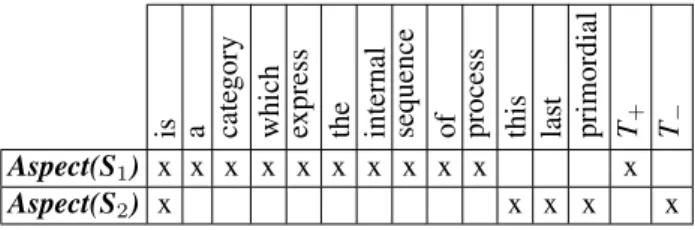
by means of the attributes shared by objects. Formally, this theory is based on the triple K = (G, M, I) called formal context, where G is a set of objects, M is a set of attributes and I is the the binary relation I ⊆ G×M between objects and attributes. Therefore, (g, m) ∈ I means that g has the attribute m. For instance, occurrences of the introductory examples with the T C Aspect are encoded in the formal context given by Table ??. A more detailed and formal de-scription of the method and its results for ambiguity diag-nosis are given in (Melo-Mora and Toussaint, 2015).
is a cate
gory
which express the internal sequence of process this last primordial T+ T− Aspect(S1) x x x x x x x x x x x
Aspect(S2) x x x x x
Table 1: An example of formal context where each row rep-resents one occurrence of the T C Aspect with the words appearing in its neighbourhood
Hypotheses are computed for each T C separately. For each T C, a set of positive and a set of negative hypotheses are built. First, each T O and N T O is described by its textual context, i.e. the words in the sentence. The occurrence is a “positive example” (belonging to the “T+class”) if it is a
T O or a “negative example” (“T−class”) if it is a N T O. A
positive (resp. negative) hypothesis is an itemset of words corresponding to positive (resp. negative) occurrences of a T C.
With regard to FCA theory, this classification method can be described by three sub-contexts : a positive con-text K+ = (G+, M, I+), a negative context K− =
(G−, M, I−), and an undetermined context Kτ =
(Gτ, M, Iτ) that contains instances to be classified. M is
a set of attributes (surrounding words), T is the target at-tribute and T /∈ M , G+ is the set of positive examples
whereas G−is the set of negative examples. Alternatively,
Gτdenotes the set of new examples to be classified.
A positive hypothesis H+for T is defined as a non empty
set of attributes of K+ which is not contained in the
de-scription of any negative example g ∈ G−. A negative
hypothesisH−, is defined accordingly. A positive
hypoth-esis H+generalizes G+subsets and defines a cause of the
target attribute T . In the best case, the membership to G+
supposes a particular attribute combination (one hypothe-sis). However, in most cases it is necessary to find several attribute combinations i.e. several positive hypotheses to characterize G+ examples. Ideally, we would like to find
enough positive hypotheses to cover all G+examples. To
reduce the number of hypotheses and in accordance with FCA, an hypothesis is a closed itemset: it corresponds to the maximal set of words shared by a maximal set of occur-rences.
Thereby, hypotheses can be used to classify an undeter-mined example. If the description of x (i.e. words in the same sentence as x) contains at lest one positive hypothesis and no negative hypothesis, then, x is classified as a posi-tive example. If the intent of x contains at least one negaposi-tive
hypothesis and no positive hypothesis, then it is a negative example. Otherwise, x remains unclassified. It should be mentioned that several alternative strategies could manage these unclassified examples such as assigning an arbitrary positive or negative class. It could improve precision or re-call but would contribute to confusing the analysis of the results.
In addition, we can restrict the number of useful hypotheses with regard to subsumption in the lattice. Formally, a posi-tive hypothesis H+is a minimal positive hypothesis if there
is no positive hypothesis H such that H ⊂ H+. Minimal
negative hypothesisis defined similarly. Hypotheses which are not minimal should not be considered for classification because they do not improve discrimination between posi-tive and negaposi-tive examples.
4.3.
Lafon’s Specificity Approach (LS)
This approach relies on a statistical analysis following La-fon’s model of specificity (Lafon, 1980; Drouin, 2007). Two sets of lexical components are extracted from the train-ing corpus: for each T C, a set of lexical contexts for its T O, the other one for its N T O.
The terminological set and the non-terminological set are built as follows:
• For each T C occurrence in the training corpus, if it is a T O (resp. N T O), store the lexical components of its linguistic context (the paragraph as it is marked by the well-known XMLtag <p>) to the terminological (resp. non terminological) set;
• In each set, for each lexical unit, compute the speci-ficity score. It reflects the over-representation or the under-representation of the unit inside each set in com-parison with the whole corpus. This score is computed with the TXMtool (Heiden et al., 2010);
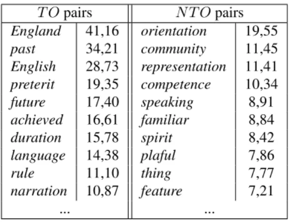
• Finally, each set contains pairs (lexical unit, specificity score). In Table 2, some of the most specific compo-nents of the terminological (resp. non-terminological) sets which are computed for the T C aspect on the training corpus are reproduced here.
T O pairs N T O pairs England 41,16 orientation 19,55 past 34,21 community 11,45 English 28,73 representation 11,41 preterit 19,35 competence 10,34 future 17,40 speaking 8,91 achieved 16,61 familiar 8,84 duration 15,78 spirit 8,42 language 14,38 plaful 7,86 rule 11,10 thing 7,77 narration 10,87 feature 7,21 ... ...
Table 2: Lafon’s Specificity: most specific components of the terminological (resp. non-terminological) sets for the T C aspect
The terminological pairs may lead to the conclusion that most papers in which aspect occurs with its linguis-tic meaning (the T O) are dealing with applied linguislinguis-tics for non native speakers. By contrast, the diversity of the non-terminological pairs may only lead to the conclusion that papers in which aspect occurs with one of its non-terminological meanings, for instance a specific facet for a given issue, are dealing with many other issues.
But these sets are not intended to provide a meaningful rep-resentation of T O (resp. N T O) of the T C aspect. There are only used to decide, for each T C occurrence, if it is closer to T O (resp. N T O) of aspect following the sets which have been computed with the training corpus. In the test corpus, the linguistic context of each T C occur-rence is compared to these two sets.
The method selects the set with the most significant inter-section: the largest number of units in common with the highest specificity score.
For instance, the following occurrence of aspect L’aspect, cat´egorie par laquelle l’ ´enonciateur conc¸oit le d´eroulement interne d’ un proc`es, est marqu´e en cr´eole ha¨ıtien au moyen de particules marqueurs pr´edicatifs MP pr´epos´ees au verbe. (’Aspect, category by which the speaker con-veives the internal workflow of a process, is marked in Haitian Creole by means of parti-cles predicative markers MP which precede the verb.’)
is considered as an T O because the intersection with the computed pairs on training corpus is more significant with T O pairs. Some of the most specific components which are shared are present, workflow, to express, past, duration, language, to speak, etc..
By contrast, the following occurrence of aspect L’aspect diff´erentiel c`ede la place `a une vision positive substantielle du lexique. (’The differen-tial aspect give away to a positive substandifferen-tial vi-sion of the lexicon.’)
is considered as an N T O because the intersection with the computed pairs on training corpus is more significant with N T O pairs. Some of the most specific components which are shared are orientation, relative, specific, spirit, commu-nity, unpublished, common, representation, etc..
4.4.
Salience Approach (SA)
For term disambiguation, all generic machine learning clas-sification algorithms are applicable: discriminative rithms such as C4.5 (Quinlan, 1993) or aggregative algo-rithms such as Naives Bayes. In this approach, the features are the POS tag of the T C, its lemma and discourse clues that rely on text genre properties called salience ((Brixtel et al., 2013; Lejeune and Daille, 2015)). The assumption is that T O are more often used in salient positions.
Scientific texts contains only a few important terms. These terms appear in salient positions in order to ease the un-derstanding of the reader. When an important term oc-curs it comes along with other important terms in a gre-garious manner. On the contrary, N T Os are more equally
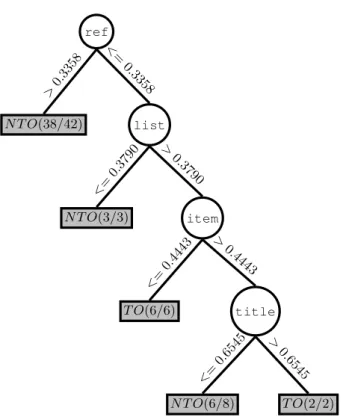
ref N T O(38/42) >0. 3358 list N T O(3/3) <= 0.3790 item T O(6/6) <= 0.4443 title N T O(6/8) <= 0.6545 T O(2/2) > 0.6545 > 0.4443 > 0.3790 < = 0.3358
Figure 1: Decision Tree computed for occurrences of the T C Aspect: each node is an XMLtag and each edge ex-hibits the normalized distance between on occurrence and the closest tag of this type, for each decision (T O or N T O), the proportion of True Positives is given
distributed within the document. Furthermore, the num-ber of salient positions is limited so that it is unlikely that N T Os will occupy salient positions rather than other posi-tions. The discourse features are salient positions that are computed by taking advantage of the XMLstructure. The main tags found in our corpus are :
text the full text, including its title and its body ; div a section with head its title and p its paragraphs ; list a bulleted list with item its items;
keywords keywords given by authors ; ref reference to bibliography.
An example of a decision tree obtained for the term Aspectis given in Figure 1. This is a set of rules spe-cific to occurrences of this T C that are not classified using generic rules. This example shows for instance that occur-rences of Aspect are very unlikely to be T Os when they are not close to bibliographical references represented by the ref tag (Node 1).
For each T C, the position is computed as follows: • For each XMLtag type in the document:
– Compute the distance (in characters) between the T C and the closest tag of this type;
– Normalize this distance with respect to the length of the text. POL ROL HB LS SA DR 78.8% 100% 53.5% 71.8% 100% P 69.8% 66.2% 84.9% 69.1% 73.0% F NA 5398 9841 2374 4996 6634 RA 59.8% 53.1% 78.9% 66.9% 68.4% F1A 64.4% 59.0% 81.8% 67.9% 70.6% F0.5A 65.4% 60.3% 82.48% 68.2% 71.1% F NB 12955 9841 12125 10914 6634 RB 38.3% 53.1% 42.2% 48.0% 68.4% F1B 49.4% 59.0% 56.4% 56.6% 70.6% F0.5B 52.5% 60.3% 60.56% 58.8% 71.1%
Table 3: Results for the two baselines, Precision Oriented (POL) and Recall Oriented (ROL) Lesk, and the three approaches: Hypotheses Based (HB), Lafon’s Specificity (LS) and Salience (SA) for the two settings
Positional features are combined with lemmas and POS tags to train a classifier. For the choice of a classifier, we rely on the work of (Yarowsky and Florian, 2002) that ob-served that discriminative algorithms such as decision trees perform better than aggregative algorithms for smaller sets of highly discriminative features, and use the default set-tings of C4.5 included in the WEKA tool (Witten and Fanck, 2005).
5.
Results
The results obtained on the test corpus are presented in Ta-ble 3. True Positives (T P s) are correctly classified T Os. False Positives (F P s) are N T Os wrongly tagged as T Os. Some of the methods (POL, LS and HB) do not give an answer for every candidate, this indecisiveness leads to un-classified T Os. This may affect computation and analysis of the recall scores. Therefore, we propose two definitions of False Negatives (F N ).
Type A False Negatives (F NA) are misclassified T Os only,
they are used for the A setting. By adding unclassified T Os and misclassified T Os, we obtain type B False Negatives (F NB), used for the B setting.
The A setting favours precision-oriented approaches that do not decide for every occurrence. On the contrary, the B set-ting favours recall-oriented approaches. We also computed the decision rate which is the number of T Os for which a decision is taken.
The measures are computed as follows:
• Decision Rate: DR = (T P + F NA)/(T P + F NB) • Precision : P = T P/(T P + F P ) • Type A Recall : RA= T P/(T P + F NA) • Type B Recall : RB = T P/(T P + F NB) • FA-measure: FβA = (1 + β 2) ∗ PA∗RA (β2∗P A)+RA • FB-measure: FβB = (1 + β 2) ∗ PB∗RB (β2∗PB)+RB
F-measure is computed with the classical setting β = 1 and with β = 0.5 to give a greater importance to precision.
6.
Discussion and Conclusion
In this section we first present an analysis of the behavior of HB and SA methods. We then compare the results given by the three methods relatively to manual annotation (MA). Analysing Hypotheses The number of positive hypothe-ses and negative hypothehypothe-ses varies a lot depending on the T C. Table 4 gives observations for five T Cs. Frequency is the number of occurrences in the training set, among them some are positive occurrences and the ratio between these two values gives the terminological degree. The ta-bles gives also the total number of surrounding words in-volved in positive (resp. negative) hypotheses and the num-ber of positive (resp. negative) hypotheses. Unsurprisingly, the number of hypotheses mainly increases (even if mono-tonicity cannot be ensured) with the number of examples. The number of hypotheses is usually much higher than the number of examples. The number of positive hypotheses varies in a non-monotonic way respectively to the termino-logical degree. However, if a term has a high terminologi-cal degree, the number of positive hypotheses is greater that the number of negative hypotheses and reciprocally for low terminological degree. When the terminological degree is around 50%, positive/negative numbers of hypotheses are rather balanced . T C Frequenc y Positi v e Occurrences Terminolog. De gree W ords used only in T+ Hypotheses Generated from
T+ Proportion of
Positi
v
e
Hypotheses Shared Words Ne
g ati v e Examples Words used only in T− Hypotheses Generated from
T− adjective216 207 95.83% 966 301 97.41% 64 9 59 8 corpus 688 510 74.12% 1035 1347 81.93% 713 178 535 297 text 568 266 46.83% 735 913 52.32% 772 302 792 832 relation 676 171 25.29% 159 183 11.48% 629 505 1427 1410 semantic413 80 19.37% 272 108 8.88% 560 333 1258 1107
Table 4: Classification summary of candidate occurrences
Results from the test phase for hypotheses are given in Ta-ble 5 for some T Cs. TaTa-ble 5 shows the average number of hypotheses used to tags T C occurrences over the different runs where Ex2tag is the average number of occurrences to be tagged for this T C.
As hypotheses are set of surrounding words, we can ob-serve what are the positive and the negative triggers for a given T C. Table 6 gives some examples of hypotheses for the T C argument. They have been ranked in decreasing order of the stability measure, a measure defined in FCA for evaluating quality of concepts in a lattice (Kuznetsov, 2007).
Analysis of the Salience Approach The POS tag feature is usually very useful when a T C can be an adjective or a noun: when a T C is an adjective, it is more likely to be a N T O. For instance, radical as an adjective is a N T O in 90% of times while it is a T O in 80% of times when it is a noun. Another interesting example is the T C linguistique (linguistics), its occurrences in the be-ginning of a paragraphs are always T Os. The classification of its other occurrences implies rules combining the POS tag feature and the salience features.
Hypotheses used Unclassified examples T C Term. Degree Ex2tag positive negative positive negative adjective 95.83% 27 46 0 1.375 0.125
corpus 74.12% 86 268 61 25.5 5.25
text 46.83% 71 194 145 7.625 5.75
relation 25.29% 142.25 16 244 1.5 9.5 semantic 19.37% 51.62 20 288 0.5 5.5
Table 5: Average for all the runs of hypotheses used in test and unnamed examples in k-fold cross-validation (k = 8)
Support Stability Hypotheses in T+ Hypotheses in T+
-english-Positive Hypotheses
7 0.7968 [sdrt, ˆetre, argument] [sdrt, be, argument] 9 0.7792 [argument, plus] [argument, more] 6 0.73437 [ˆetre, argument, aussi] [be, argument, also] 6 0.7187 [argument, verbal] [argument, verbal] . . . .
5 0.6562 [ˆetre, argument, indique] [be, argument, denote] 4 0.5 [argument, syntaxique] [argument, syntactic] . . . .
6 0.3281 [ˆetre, argument, rst] [be, argument, rst] 8 0.25 [argument, nucleus] [argument, nucleus]
Negative Hypotheses
3 0.5 [argument, prendre] [argument, assume] 1 0.5 [trancher, pas, ne, argument,
permettre, d´ecisif, position, avoir]
[settle, not, argument, allow, decisive, position, have] . . . .
4 0.375 [argument, hypoth`ese] [argument, hypothesis] 4 0.3125 [dire, argument] [say, argument] . . . .
2 0.25 [trouver, mˆeme, argument] [find, same, argument]
Table 6: Some positive and negative hypotheses for the argumentcandidate term
In order to ease comparisons with the hypothesis-based method, Table 6. exhibits some results for the T C semanticalready analyzed in Table 5. Less than 20% of its occurrences are T Os, they are equally distributed among the two POS tags but 77% of T Os as a noun whereas it is the case only for 15% of its occurrences as an adjec-tive. These examples were found in weakly structured doc-uments with few references and very long sections. These are critical cases for our method when neither the POS tag nor structural features give enough information for the clas-sification. The method still gives a diagnosis but is not reli-able.
Analysis of the Results We can see an important differ-ence when examining the performances in the two settings. In the A setting, the HB approach gives the best results thanks to its greater precision. The two baselines are performed: their type A recall is low and precision is out-performed by both SA and HB approaches. Conversely,
Res POS title head p item ref FN ADJ 0.8131 0.5064 0.1914 0.8079 0.4875 FN NOUN 0.8324 0.5439 0.1116 0.8279 0.1516 TN ADJ 0.8368 0.5483 0.1160 0.8323 0.1472 TP NOUN 0.8406 0.5717 0.1636 0.8318 0.0342 TN ADJ 0.8523 0.5638 0.1315 0.8478 0.1317
Table 7: Examples of good and bad classification of the T C semantic
Confidence Support Association rule (in %) (in %)
0.93 0.31 [HB-NTO, LS-NTO] −→ [SA-NTO] 0.93 0.28 [MA-NTO, HB-NTO, LS-NTO] −→ [SA-NTO] 0.93 0.1 [HB-TO, LS-TO] −→ [SA-TO] 0.93 0.09 [MA-TO, HB-TO, LS-TO] −→ [SA-TO] 0.92 0.33 [MA-NTO, HB-NTO] −→ [SA-NTO] 0.92 0.13 [MA-TO, HB-TO] −→ [SA-TO] 0.91 0.4 [MA-NTO, LS-NTO] −→ [SA-NTO] 0.91 0.36 [HB-NTO] −→ [SA-NTO]
0.91 0.28 [SA-NTO, HB-NTO, LS-NTO] −→ [MA-NTO] 0.91 0.16 [HB-TO] −→ [SA-TO]
0.91 0.09 [MA-NTO, HB-UN, LS-UN] −→ [SA-NTO] 0.9 0.36 [HB-NTO] −→ [MA-NTO] 0.9 0.33 [SA-NTO, HB-NTO] −→ [MA-NTO] 0.9 0.3 [HB-NTO, LS-NTO] −→ [MA-NTO] 0.9 0.11 [MA-NTO, HB-UN, LS-NTO] −→ [SA-NTO] 0.89 0.15 [MA-TO, LS-TO] −→ [SA-TO] 0.89 0.11 [MA-NTO, LS-UN] −→ [SA-NTO] 0.88 0.4 [SA-NTO, LS-NTO] −→ [MA-NTO] 0.88 0.05 [MA-TO, HB-UN, LS-TO] −→ [SA-TO]
. . . .
0.85 0.11 [SA-NTO, HB-UN, LS-NTO] −→ [MA-NTO] 0.85 0.09 [SA-TO, HB-TO, LS-TO] −→ [MA-TO]
. . . .
0.7 0.09 [SA-NTO, HB-UN, LS-UN] −→ [MA-NTO]
. . . .
Table 8: Some best-confidence association rules between annotations
the B setting favours methods with a higher decision rate. It should be noticed that no strategy has been implemented yet to compute a value when our algorithms (LS and HB) are in a situation of indecisiveness while our Lesk version uses one.
We performed a more fine-grained comparison of the re-sults of the approaches, occurrence per occurrence. Each occurrence of a T C, whatever the T C is, is described by a set of four multi-valued attributes (the four different annotations) corresponding the manual annotations (MA), the hypotheses-based annotations (HB), Lafon’s specificity (LS) and Salience (SA) annotations. Among 59,168 oc-currences, 24,964 are not classified by HB, and 13,615 are not classified by LS. 10,230 are not classified by these two approaches. Among these 10,230 occurrences, 1,988 are T O correctly classified by SA, 5,549 are N T O correctly classified by SA, and 2,287 are T O wrongly classified by SA.
To study links between the different methods, we also ex-tracted association rules between the diagnosis given by the different methods. Each occurrence of T C has been de-scribed following this example :
#d1e2267-definition : MA-NTO, SA-NTO, HB-UN, Laf-UN This can be read as follows:
• the identifier of the occurrence: this is the occurrence with the ID #d1e2267 of the T C definition; • the manual annotation (M A), salience annotation
(SA), hypotheses annotation (HB) and Lafon’s speci-ficity annotation (LS)
• and the value of the annotation: non-terminological (NTO), terminological(TO) or unknown (UN)
An association rule of the type :
confidence =0.93, support =0.1, [HB-TO, LS-TO] −→ [SA-TO]
means that if HB and LS annotates an occurrence as a T O then SA will do so in 93% of the cases (confidence) and it concerns 5916 occurrences, i.e. 10% (support) of the total number of the occurrences (59,168).
We extracted 86 association rules with a confidence higher than 50% and a support higher than 5% (2956 occur-rences). Table 8 shows some of the best-confidence rules. One should be aware that association rules do not ex-press causality but only observations between annotations. Among these association rules, let us give a focus on :
• 0.91, 0.4, [MA-NTO, LS-NTO] −→ [SA-NTO] means that when M A and LS annotates an occurrence as N T O, then SA mostly does so.
• 0.91, 0.36, [HB-NTO] −→ [SA-NTO] means that if HB gives a N T O diagnosis then SA mostly does so. • 0.91, 0.28, [SA-NTO, HB-NTO, LS-NTO] −→ [MA-NTO] means that if the three methods agree on a N T O diagnosis, then generally M A is N T O. • 0.91, 0.16, [HB-TO] −→ [SA-TO] means that if HB
gives a T O diagnosis, then SA mostly does so. • 0.85, 0.11, [SA-NTO, HB-UN, LS-NTO] −→
[MA-NTO] means that if SA and SL agree on a N T O di-agnosis, then probably M A is N T O.
• 0.85, 0.09, [SA-TO, HB-TO, LS-TO] −→ [MA-TO] means that if our three methods agree on a T O anno-tation for an occurrence, then generally M A is T O. • 0.7, 0.09, [SA-NTO, HB-UN, LS-UN] −→
[MA-NTO] means that when SA gives a N T O diagnosis when HB and LS cannot take decision, then it is not always a good diagnosis (confidence is only 0.7). Conclusion In this paper, we presented a dataset de-signed for an ambiguity diagnosis task. We evaluated three methods and two baselines derived from the Lesk algo-rithm. We pointed out that a difficulty for evaluating this task is the impact of two different types of F N s: misclas-sified items VS unclasmisclas-sified items. We showed that this has a great impact on evaluation.
In future work, we will combine the different methods in or-der to take advantage of their different properties in terms of confidence (precision) and coverage (recall). We observed that a combination of our three methods of annotation that roughly favours T O annotations will pull down precision very close to the worst precision of the three methods and will provide a very low improvement of recall. Thus, asso-ciation rules could probably suggest a better combination of these three methods.
7.
References
R. Brixtel, G. Lejeune, A. Doucet, and N. Lucas. 2013. Any Language Early Detection of Epidemic Diseases from Web News Streams. In International Conference on Healthcare Informatics (ICHI), pages 159–168. D. Cothire-Robert. 2007. Strat´egies des restitutions des
constructions verbales s´erielles du cr´eole hatien en franais l2. In Autour des langues et du langage: perspec-tive pluridisciplinaire. Presses Universitaires de Greno-ble.
B. Daille, C. Jacquin, L. Monceaux, E. Morin, and J. Ro-cheteau. 2011. TTC TermSuite : une chaˆıne de traite-ment pour la fouille terminologique multilingue. In 18`eme Conf´erence francophone sur le Traitement Au-tomatique des Langues Naturelles Conference (TALN 2011)., Montpellier, France, June. D´emonstration. P. Drouin. 2007. Identification automatique du lexique
sci-entifique transdisciplinaire. Revue franc¸aise de linguis-tique appliqu´ee, 12(2):45–64.
T. El-Khoury. 2007. Les proc´ed´es de m´etaphorisation dans le discours m´edical arabe : ´etude de cas. In Autour des langues et du langage: perspective pluridisciplinaire. Presses Universitaires de Grenoble.
J. Foo and M. Merkel. 2010. Using machine learning to perform automatic term recognition. In N´uria Bel, B´eatrice Daille, and Andrejs Vasiljevs, editors, LREC 2010 Workshop Methods for the automatic acquisition of Language Resources and their evaluation methods, pages 49–54, Malta.
B. Gaiffe, B. Husson, E. Jacquey, and L. Kister. 2015. Smarties: Consultation des fichiers annot´es manuellement, domain scientext 2014, available at http://apps.atilf.fr/smarties/index.php?r=text/listtext. S. Heiden, J-P. Magu´e, and B. Pincemin. 2010. Txm : Une
plateforme logicielle open-source pour la textom´etrie conception et d´eveloppement. In Proceedings of JADT 2010 : 10th International Conference on the Statistical Analysis of Textual Data, page 12pp, Rome, Italie. A. Judea, H. Sch¨utze, and S. Bruegmann. 2014.
Unsu-pervised training set generation for automatic acquisi-tion of technical terminology in patents. In Proceed-ings of COLING 2014, the 25th International Conference on Computational Linguistics: Technical Papers, pages 290–300, Dublin, Ireland, August. Dublin City Univer-sity and Association for Computational Linguistics. S. O. Kuznetsov. 2001. Machine learning on the basis
of formal concept analysis. Autom. Remote Control, 62(10):1543–1564.
S. O. Kuznetsov. 2004. Complexity of learning in concept lattices from positive and negative examples. Discrete Applied Mathematics, 142(13):111 – 125. Boolean and Pseudo-Boolean Functions.
Sergei O Kuznetsov. 2007. On stability of a formal con-cept. Annals of Mathematics and Artificial Intelligence, 49(1-4):101–115.
P. Lafon. 1980. Sur la variabilit´e de la fr´equence des formes dans un corpus. Mots, 1:127–165.
G. Lejeune and B. Daille. 2015. Vers un diagnostic d’ambigu¨ıt´e des termes candidats d’un texte. In Actes
de la 22e conf´erence sur le Traitement Automatique des Langues Naturelles (TALN’2015), pages 446–452. M. Lesk. 1986. Automatic sense disambiguation using
ma-chine readable dictionaries: How to tell a pine cone from an ice cream cone. In Proceedings of the 5th Annual In-ternational Conference on Systems Documentation, SIG-DOC ’86, pages 24–26, New York, NY, USA. ACM. M.-C. L’Homme. 2004. La terminologie : principes et
techniques. Presses de l’Universit de Montral.
L.-F. Melo-Mora and Y. Toussaint. 2015. Automatic vali-dation of terminology by means of formal concept anal-ysis. In International Conference on Formal Concept Analysis (ICFCA).
R. Navigli. 2009. Word sens disambiguation: A survey. ACM Computing Surveys, 41(2).
J. R. Quinlan. 1993. C4.5: programms for machine learn-ing. Morgan Kaufmann Publishers, San Francisco, CA, USA.
A. Tutin and F. Grossmann. 2015. Scientext: Un corpus et des outils pour ´etudier le positionnement et le raisonnement dans les ´ecrits scientifiques, available at http://scientext.msh-alpes.fr/scientext-site/spip.php?article8.
I. H. Witten and E. Fanck. 2005. Data Mining: Practical Machine Learning Tools and Techniques. Morgan Kauf-mann, San Francisco.
D. Yarowsky and R. Florian. 2002. Evaluating sense dis-ambiguation across diverse parameter spaces. Natural Language Engineering, 8(4):293–310.