Damage Detection of Mechanical Components Using Null Subspace Analysis

(1)

DAMAGE DETECTION OF MECHANICAL COMPONENTS USING NULL

SUBSPACE ANALYSIS

C. Rutten*, C. Loffet**, J.C. Golinval*

*University of Liège, Department of Mechanical Engineering, LTAS-Vibrations et Identification

des Structures

*Chemin des Chevreuils 1, 4000 Liège, Belgium

**V2i sa

**Liège Science Park, Rue des Chasseurs Ardennais 4, 4031 Angleur, Belgium

e-mail:

christophe.rutten@ulg.ac.be

,

jc.golinval@ulg.ac.be

Abstract: This paper presents two original applications of the Null Subspace Analysis (NSA) method for fault

diagnosis in mechanical components. The method is first applied to the case-study of electro-mechanical devices at the end of the assembly line with the aim of assessing their overall quality. The advantages of the proposed method rely in its rapidity of use and its reliability. At first, a set of five good (i.e. healthy) devices and four damaged devices was considered. The components were instrumented with one triaxial accelerometer on the flank and one monoaxial accelerometer on the top. Based on the NSA method, a mapping of the space [ active components, system order ] up to a system order of 100, was realized in order to select the appropriate order and number of active components. Eventually, thanks to this mapping, the method was able to successfully detect all the faulty components using the signal from only one accelerometer in one direction. The second application is related to the quality assessment of welded joints between stripes in a steel processing plan. Six welded joints with nominal welding parameters and twenty-seven welded joints with out-of-range parameters were realized. Again, the NSA method was able to diagnose successfully the welded joints using a single signal from one accelerometer.

Keywords: Quality assurance, damage detection, Null Subspace Analysis Introduction

The quality control process of a mechanical component at the end of the production line is time consuming and may slow down the production process. Hence only a few samples of the components are usually tested and it may happen that faulty components are provided to the customer. That is why a quick, simple and reliable check of quality at the end of the assembly line is highly desirable.

In this paper, the Null Subspace Analysis (NSA) method is applied to two industrial cases. The method is first applied to a set of nine electro-mechanical rotating devices. NSA uses a reference vibration signal measured on a randomly chosen healthy component and compares its dynamics to the dynamics of the signal measured on the other components.

The method is afterwards applied to the quality assessment of welded joints between two stripes in a steel processing plan.

NSA has already been successfully used for damage detection in bearings [1] and on an airplane mock-up [2].

1. Null Subspace Analysis

Null Subspace analysis is basically a principal component analysis of the Hankel autocorrelation matrix which is defined as follows [2]:

(1)

where p and q are user-defined parameters (p = q in this paper) and represents the output covariance matrix defined by:

(2)

where yk is the measurement vector at time step k and N

(2)

It can be shown that this matrix characterizes the dynamics of the analyzed signal [1].

Performing a Singular Value Decomposition of the Hankel matrix, we obtain the following relationship [2,3]:

(3)

where U is an orthonormal matrix, each column representing a principal component, S is a diagonal matrix of singular values (ordered in decreasing order), and V is the time evolution of the amplitude of each principal component.

The small singular values which correspond to principal components of low “energy” are usually associated to noise or to weak dynamics that may be neglected. Hence, the U matrix can be factorized in two subspace, namely the active ( and the null subspace ( ) [2]:

(4) The number of components in the active subspace is user-defined. It should be chosen such that the dynamics of the signal is accurately modeled without accounting for the background noise. A usual rule of thumb is to choose a number of active components such that their cumulated “energy” represents 90% of the total “energy”. In this paper we use an alternative procedure to choose the number of active components, based on the mapping of the whole space [active components – size of the Hankel matrix].

2. Damage detection

Two damage indicators can be built using the active and null subspace of the autocorrelation matrix. The first indicator is based on the concept of angles between two subspaces. It can be show that the following equation is always true for any given dataset [2]:

(5) So, let us assume that the column null subspace, ,has been determined for a reference dataset. Now consider the column active subspace of the ith dataset. The previous relationship applies with some residue, :

(6)

This residue matrix may be chosen as candidate for damage-sensitive indicator.

The second indicator is based on the reconstruction error of the Hankel autocorrelation matrix (better known as “Novelty Analysis”) [4]. This time, let’s assume that the active subspace has been determined for the reference dataset. Now, let us try to reconstruct the Hankel correlation matrix of the ith dataset, using the reference active components and let’s define the reconstruction error

(7) (8) If the reconstruction error is significant, the reference active subspace does not represent accurately the dynamic of the analyzed signal. The Mahalanobis norm of the reconstruction is used as damage-sensitive feature:

(9) with , the covariance of the Hankel matrix.

3. First application - Experimental setup

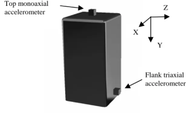
A set of nine rotating devices was instrumented with two accelerometers: one triaxial accelerometer was located on the flank of the component, and one monoaxial on the top as illustrated in Figure 1. Among this set of nine devices, four of them are known to be faulty and the other five are heathy.

Fig. 1 Locations of the accelerometers on the analysed devices: one monoaxial accelerometer on the top and one tri-axial

accerometer on the flank of the device

A total of 4 915 200 points with a sampling frequency of 20 480 Hz were measured on each channel using the LMS Scadas III acquisition system (Figure 2).

Top monoaxial accelerometer Flank triaxial accelerometer X Z Y

(3)

Fig. 2 LMS aquisition system

4. First application - Results

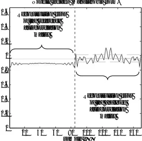
In this section, we use the second damage indicator based on the reconstruction error of the autocorrelation matrix. In order to characterize the reconstruction error, we computed the percentage of errors above a user-defined limit. This limit was set to the 6 σ-limit defined on the reconstruction error of the reference autocorrelation matrix.

20 40 60 80 100 120 140 160 0 0.2 0.4 0.6 0.8 1 1.2 1.4 1.6 sample n°

Novelty indices (Mahalanobis norm)

Fig. 3 Novelty index overshoot with the 6 σ-limit in solid line

In order to select the appropriate size of the Hankel matrix and the appropriate number of active components, a mapping of the space [number of principal component, system order] was realised, up to system order 100.

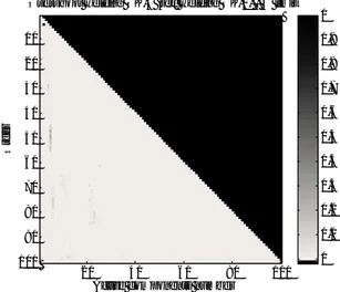
Figure 4 shows the mapping of the overshoot indicator for one healthy device in the X direction of the flank sensor. It is observed that some regions of the picture (in the range up to 10 active components) present significant overshoot. These regions should be disregarded for fault detection purpose as they would lead to false-positive alarms.

Overshoot Device OK-1 (ref: Device OK-0) X-direction

Active components number

O rder 20 40 60 80 100 10 20 30 40 50 60 70 80 90 100 0 0.1 0.2 0.3 0.4 0.5 0.6 0.7 0.8 0.9 1

Fig. 4 Mapping of a healthy component in the X direction using 6 sigmas limit

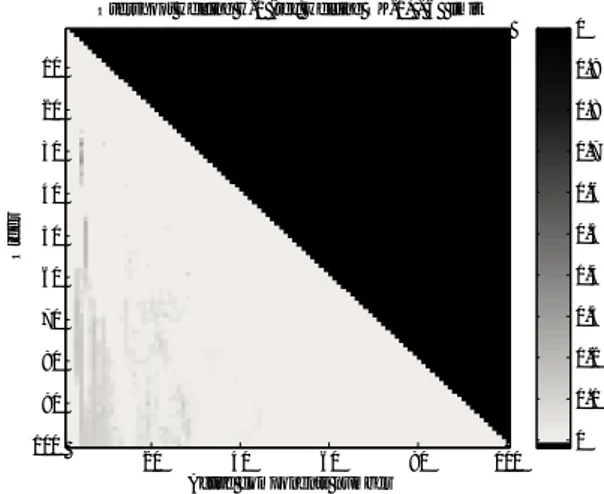
Figure 5 shows the mapping for a damaged device in the X direction again. It is observed that the regions where the overshoot is significant are totally different than in the case of the healthy component. We can also note that using high system order (above 50) may be interesting.

Overshoot Device NOK-2 (ref: Device OK-0 ) X-direction

Or d e r 20 40 60 80 100 10 20 30 40 50 60 70 80 90 100 0 0.1 0.2 0.3 0.4 0.5 0.6 0.7 0.8 0.9 1

Fig. 5 Mapping of a damaged component in the X direction using 6 sigmas limit

Figures 6 and 7 present the results in the Y direction. We note that the regions with significant overshoots in Figure 7 (faulty component) are clearly different than the ones in Figure 6 (healthy component).

Reconstruction error of the reference autocorrelation matrix Reconstruction error of the analyzed autocorrelation matrix

(4)

Overshoot Device OK-1 (ref: Device OK-0) Y-direction

Or d e r 20 40 60 80 100 10 20 30 40 50 60 70 80 90 100 0 0.1 0.2 0.3 0.4 0.5 0.6 0.7 0.8 0.9 1

Fig. 6 Mapping of a healthy component in the Y

direction using 6 sigmas limit

Overshoot Device NOK-2 (ref: Device OK-0) Y-direction

Or d e r 20 40 60 80 100 10 20 30 40 50 60 70 80 90 100 0 0.1 0.2 0.3 0.4 0.5 0.6 0.7 0.8 0.9 1

Fig. 7 Mapping of a damaged component in the Y

Figures 8 and 9 show the results for the Z direction. Because of the poor sensitivity of the indicator in this direction, we used the 3 limit instead of the 6 σ-limit. We note that in this direction, we do not have a clear separation between the high overshoot regions associated with the healthy and faulty devices respectively.

Overshoot Device OK-1 (ref: Device OK-0) Z-direction

Or d e r 20 40 60 80 100 10 20 30 40 50 60 70 80 90 100 0 0.1 0.2 0.3 0.4 0.5 0.6 0.7 0.8 0.9 1

Fig. 8 Mapping of a healthy component in the Z

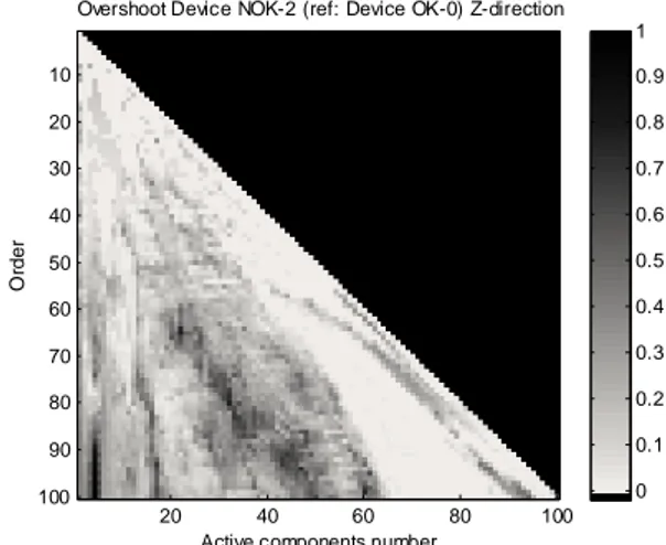
Overshoot Device NOK-2 (ref: Device OK-0) Z-direction

Or d e r 20 40 60 80 100 10 20 30 40 50 60 70 80 90 100 0 0.1 0.2 0.3 0.4 0.5 0.6 0.7 0.8 0.9 1

Fig. 9 Mapping of a damaged component in the Z

Finally Figures 10 and 11 show the mapping of the top accelerometer of a healthy device. Major overshoot can be noticed in the central area of the graph in both cases. Probably, another indicator than the overshoot would have given better results in this case.

(5)

Overshoot Device OK-1 TOP (ref: Device OK-0 TOP)

O rder 20 40 60 80 100 10 20 30 40 50 60 70 80 90 100 0 0.1 0.2 0.3 0.4 0.5 0.6 0.7 0.8 0.9 1

Fig. 10 Mapping of a healthy component, top accelerometer, 6 sigmas limit

Overshoot Device NOK-2 TOP (ref: Device OK-0 TOP)

Or d e r 20 40 60 80 100 10 20 30 40 50 60 70 80 90 100 0 0.1 0.2 0.3 0.4 0.5 0.6 0.7 0.8 0.9 1

Fig. 11 Mapping of a damaged component, top accelerometer, 6 sigmas limit

According to the previous mapping results, the fault detection procedure based on the Novelty Analysis index was applied for each device.

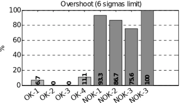
Figures 12, 13, 14 and 15 give the final results for, the X direction, the Y direction, the Z direction and the top accelerometer respectively. The results were obtained using only a time measurement sample of 30 seconds. We can see that the results are good especially in the Y direction. 0 20 40 60 80 100 %

Overshoot (6 sigmas limit)

7. 1 9. 5 4. 8 4. 8 26 .2 61 .9 45 .2 92 .9 OK-1OK-2OK-3OK-4_NO K-1 NO K-2 NO K-3 NO K-4

Fig. 12 Overshoot indicator for each analyzed device, in the X direction – order 84, 22 active components

0 20 40 60 80 100 %

6. 7 0 0 11 .1 93 .3 86 .7 75 .6 10 0 OK-1OK-2OK-3OK-4_NO K-1 NO K-2 NO K-3 NO K-3

Fig. 13Overshoot indicator for each analyzed device, in the Y direction – order 90, 80 active components

0 10 20 30 40 50 %

0 0 0 0 24 45 .3 34 .7 10 .7 OK-1OK-2OK-3OK-4_NO K-1 NO K-2 NO K-3 NO K-4

Fig. 14Overshoot indicator for each analyzed device, in the Z direction – order 75, 68 active components

0 20 40 60 80 100 %

6. 7 0 40 46 .7 10 0 86 .7 66 .7 80 OK-1OK-2OK-3 OK-4 NO K-1 NO K-2 NO K-3 NO K-4

Fig. 15Overshoot indicator for each analyzed device, top accelerometer – order 30, 25 active components 5. First application - Discussion

We want to emphasize the fact that the proposed mapping is related to one specific device only. Hence, although this mapping gives interesting clues on what

(6)

association of system order and number of active components to choose, we still need to use a trial and error approach the select the best combination.

Using high system order appears to be useful. It is particularly clear in Figure 5 where no significant overshoot can be seen at orders below 50.

6. Second application – Experimental setup

In this section, another industrial application of the NSA method is presented. An industrial welding machine from a steel processing plan was instrumented with a monoaxial accelerometer on the forging wheel (as illustrated in figure 16). The purpose of this wheel is to flatten the welded joint.

Fig. 16 Location of the accelerometer on the forging wheel of the welding machine

Vibration measurements were acquired during the whole welding process (about 3 seconds) at a sampling frequency of 25600 Hz using a National Instrument data acquisition device.

The quality of the weld depends on several parameters. During the measurement campaign, six welded joints were realized using nominal welding parameters and 27 joints were realized using out-of- range parameters. In this example, four parameters were altered and three welds were realized with each modified parameter (see Table 1).

Modified

parameter First alteration Second alteration Covering -33% (welding A) -66% (welding B) Compensation -33% (welding C) -66% (welding D) Current -10% (welding E) -20% (welding F) Forging

pressure -10% (welding G) +5% (welding H) Covering and

Compensation -66% (welding I)

Table 1 Welds realized with altered parameters (with respect to the nominal parameters).

A microscopic quality control of each welded joint was realized after the measurement campaign. Welded joints realized with nominal parameters as well as welded joints C and G were diagnosed good, welded joints named A, D, E, H were diagnosed acceptable, and welded joints B, F, I were diagnosed bad.

7. Second application – Results

Based on the NSA method, a mapping of the space [number of active component, order of the Hankel matrix] was realized in order to select the appropriate order and number of active components. The reference welded joint corresponds to the first weld realized with the nominal parameters.

Figure 17 shows the mapping related to another welded joint with nominal parameters while Figure 18, 19, 20, 21 shows the mapping of welded joints realized with altered welding parameters.

Overshoot welding OK-5 (ref: welding OK-1) - 6σ limit

O rder 20 40 60 80 100 10 20 30 40 50 60 70 80 90 100 0 0.1 0.2 0.3 0.4 0.5 0.6 0.7 0.8 0.9 1

Fig. 17Mapping of a weld with nominal parameters

Overshoot welding B-1 (ref: welding OK-1) - 6 σ limit

O rder 20 40 60 80 100 10 20 30 40 50 60 70 80 90 100 0 0.1 0.2 0.3 0.4 0.5 0.6 0.7 0.8 0.9 1

Fig. 18 Mapping of a weld with altered parameter (Covering -66%)

(7)

Overshoot welding D-1 (ref: welding OK-1) - 6 σ limit

O rder 20 40 60 80 100 10 20 30 40 50 60 70 80 90 100 0 0.1 0.2 0.3 0.4 0.5 0.6 0.7 0.8 0.9 1

Fig. 19Mapping of a weld with altered parameter (Compensation -66%)

Overshoot welding F-1 (ref: welding OK-1) - 6 σ limit

O rder 20 40 60 80 100 10 20 30 40 50 60 70 80 90 100 0 0.1 0.2 0.3 0.4 0.5 0.6 0.7 0.8 0.9 1

Fig. 20Mapping of a weld with altered parameter (Current -20%)

Overshoot welding H-1 (ref: welding OK-1) - 6 σ limit

O rder 20 40 60 80 100 10 20 30 40 50 60 70 80 90 100 0 0.1 0.2 0.3 0.4 0.5 0.6 0.7 0.8 0.9 1

Fig. 21Mapping of a weld with altered parameter (forging pressure +5%)

Based on these mappings, order 35 and a number of 4 active components were chosen. The resulting overshoot for each measurement is shown in Figure 22. Welded joints G and C are diagnosed healthy which is in good agreement with the microscopic quality control.

0 20 40 60 80 OK-1 OK-2 OK-3 OK-4 OK-5 OK-6 A-1 A-2 A-3 B-1 B-2 B-3 C-1 C-2 C-3 D-1 D-2 D-3E-1 E-2 E-3 F-1 F-2 F-3 G-1 G-2 G-3H-1 H-2 H-3I-1 I-2 I-3 %

Overshoot for each welding (6 σ lim.)

Fig. 22 Results for each realized weld - order 35, 4 active components

8. Second application – Discussion

The bad welded joints are clearly identified in figure 22. However, the value of the overshoot indicator is not always proportionnal to the severity of the defect. For instance the overshoot indicator of welds B-3 and A-2 is the same although welding of the B series were diagnosed faulty and the ones from the A series were diagnosed acceptable.

9. Conclusion

Vibration monitoring is a useful tool to diagnose fault or to detect damage in a non intrusive way but the placement of multiple sensors can be time consuming and is not always achievable in industrial applications.

The NSA method compares the dynamics of two signals. It can be used with only one sensor which is an appreciable advantage. The mapping of the whole space [number of active components, Hankel matrix order] gives some important clues on how to choose the right combination of order and number of active components.

Two industrial applications of the method have been presented. In the first one, we were able to successfully diagnose every damaged device using only 30 seconds of measurement in one direction. In the

(8)

second one, we were able to diagnose every faulty welded joints with, again, only one accelerometer.

10. References

[1] Thiry C., Yan A-M., Golinval J.C., “Damage Detection in Rotating Machinery Using Statistical Methods: PCA analysis and Autocorrelation Matrix”, Surveillance 5 CETIM Senlis 11-13 october, 2004; [2] Yan A-M., Golinval J.C., ”Null subspace based damage detection of structures using vibration measurements”, Mechanical Systems and Signal Processing 20, 611-626, 2006;

[3] Yan A-M., Kerschen G., De Boe P., Golinval J.C.,”Structural damage diagnosis under varying environmental conditions – Part 1: A linear analysis”, Mechanical Systems and Signal Processing 19, 847-864, 2005;

[4] De Boe P., ”Les éléments piezo-laminés appliqués à la dynamique des structures”, PhD Thesis, Université de Liège, 2003;