THÈSE DE DOCTORAT
de l’Université de recherche
Paris Sciences et Lettres –
PSL Research University
préparée à l’Université
Paris – Dauphine
Lois a priori non-informatives
et la modélisation par mélange
par Kaniav KAMARY
Ecole doctorale n°543
Spécialité
: Sciences
Soutenue le 15.03.2016
Composition du Jury : M. Christian P. ROBERT Université Paris-Dauphine Directeur de thèse M. Gilles CELEUX INRIA Rapporteur M. Pierre DRUILHET Université Clermont-Ferrand 2 RapporteurMme Judith ROUSSEAU Université Paris-Dauphine Membre du jury
Mme Anne PHILIPPE Université de Nantes Présidente du jury
i
Acknowledgments
I have been very fortunate throughout my thesis to be supported by internationally renowned researchers. Now I have a great opportunity to say a big thank you to persons who contributed to my professional and human formation in the doctoral stage.
I would first like to thank my PhD supervisor, Christian P. Robert, for all the support he has given me throughout my time as a student. By his scientific person-ality and his rigor, he deeply influenced me and made me more and more passionate about my work. Numerous advices in my researches, always very judicious and confidence he has manifested me, encouraged me to improve myself and to progress every day.
My deep gratitude is for Hossein Bevrani who supports me as a professor for the license and Master and advisor for the PhD. I will always be grateful for his kindness, his confidence and all the time he gave me without ever counting.
During my PhD I had the chance to work with researchers like Kerrie Mengersen, Judith Rousseau and Kate Lee as my collaborators and I want to thank them for their support and for agreeing to work with me. I think in particular of working with Kate Lee which was really rewarding.
I would like to warmly thank the team of the Kurdish Institute of Paris, Campus France and French government for their financial support and for trusting me.
I am also very grateful to have been a PhD student at CEREMADE, université Paris-Dauphine, which always provided me with a lively and intellectually stimu-lating environment to work. I would like to thank all the faculty, Robin Ryder and particularly director Olivier Glass.
I am very grateful to my examiners, Gilles Celeux, Pierre Druilhet, Judith Rousseau and Anne Philippe, for taking the time to give me such useful feedback.
I would like to thank all the people I have met and worked with during my time at université Paris-Dauphine. It is not possible to thank everyone here but I would particularly like to mention Sofia Tsepletidou, Roxana Dumitrescu, Viviana Letizia and Nicolas Baradel ... for their scientific input, discussions, and friendship over the years.
Lastly, I would like to thank my husband Bewar, my parents and my sisters who always believed in me and always offered me unconditional love and also my friends Ayoub Moradi, Serwa Khoramdel and Fateme Mohamadipoor who have supported me all these years, even from thousands of miles away.
iii
Résumé
L’une des grandes applications de la statistique est la validation et la comparai-son de modèles probabilistes au vu des données. Cette branche des statistiques a été développée depuis la formalisation de la fin du 19ième siècle par des pionniers comme Gosset, Pearson et Fisher. Dans le cas particulier de l’approche bayésienne, la solution à la comparaison de modèles est le facteur de Bayes, rapport des vraisem-blances marginales, quelque soit le modèle évalué. Cette solution est obtenue par un raisonnement mathématique fondé sur une fonction de coût.
Ce facteur de Bayes pose cependant problème et ce pour deux raisons. D’une part, le facteur de Bayes est très peu utilisé du fait d’une forte dépendance à la loi a priori (ou de manière équivalente du fait d’une absence de calibration absolue). Néanmoins la sélection d’une loi a priori a un rôle vital dans la statistique bayésienne et par consequent l’une des difficultés avec la version traditionnelle de l’approche bayésienne est la discontinuité de l’utilisation des lois a priori impropres car ils ne sont pas justifiées dans la plupart des situations de test. La première partie de cette thèse traite d’un examen général sur les lois a priori non informatives, de leurs caractéristiques et montre la stabilité globale des distributions a posteriori en réévaluant les exemples de [Seaman III 2012].
Le second problème, indépendant, est que le facteur de Bayes est difficile à calculer à l’exception des cas les plus simples (lois conjuguées). Une branche des statistiques computationnelles s’est donc attachée à résoudre ce problème, avec des solutions empruntant à la physique statistique comme la méthode du path sam-pling de [Gelman 1998] et à la théorie du signal. Les solutions existantes ne sont cependant pas universelles et une réévaluation de ces méthodes suivie du développe-ment de méthodes alternatives constitue une partie de la thèse. Nous considérons donc un nouveau paradigme pour les tests bayésiens d’hypothèses et la comparaison de modèles bayésiens en définissant une alternative à la construction traditionnelle de probabilités a posteriori qu’une hypothèse est vraie ou que les données provi-ennent d’un modèle spécifique. Cette méthode se fonde sur l’examen des modèles en compétition en tant que composants d’un modèle de mélange. En remplaçant le problème de test original avec une estimation qui se concentre sur le poids de probabilité d’un modèle donné dans un modèle de mélange, nous analysons la sensi-bilité sur la distribution a posteriori conséquente des poids pour divers modélisation préalables sur les poids et soulignons qu’un intérêt important de l’utilisation de cette perspective est que les lois a priori impropres génériques sont acceptables, tout en ne mettant pas en péril la convergence. Pour cela, les méthodes MCMC comme l’algorithme de Metropolis-Hastings et l’échantillonneur de Gibbs et des approxi-mations de la probabilité par des méthodes empiriques sont utilisées. Une autre caractéristique de cette variante facilement mise en oeuvre est que les vitesses de convergence de la partie postérieure de la moyenne du poids et de probabilité a posteriori correspondant sont assez similaires à la solution bayésienne classique.
Dans la dernière partie de la thèse, nous sommes intéressés à la construction d’une analyse bayésienne de référence pour mélanges de gaussiennes par la création
d’une nouvelle paramétrisation centrée sur la moyenne et la variance de ces mod-èles, ce qui nous permet de développer une loi a priori non-informative pour les mélanges avec un nombre arbitraire de composants. Nous démontrons que la distri-bution postérieure associée à ce préalable est propre et fournissons des implémenta-tions MCMC qui exhibent l’échangeabilité attendu. L’analyse repose sur des méth-odes MCMC comme l’algorithme de Metropolis-within-Gibbs, Adaptive MCMC et l’algorithme de “Parallel Tempering”. Cette partie de la thèse est suivie par une package R nommée Ultimixt qui met en œuvre une description de notre analyse bayésienne générique de mélanges de gaussiennes unidimensionnelles obtenues par une paramétrisation moyenne–variance du modèle. Ultimixt peut être appliqué à une analyse bayésienne des mélanges gaussiennes avec un nombre arbitraire de composants, sans avoir besoin de définir la loi a priori.
Mots clés: Distribution de mélange, Loi a priori non-informative, Analyse bayési-enne, A priori impropre, Choix du modèle bayésien, Méthodes de MCMC.
v
Abstract
One of the major applications of statistics is the validation and comparing proba-bilistic models given the data. This branch statistics has been developed since the formalization of the late 19th century by pioneers like Gosset, Pearson and Fisher. In the special case of the Bayesian approach, the comparison solution of models is the Bayes factor, ratio of marginal likelihoods, whatever the estimated model. This solution is obtained by a mathematical reasoning based on a loss function.
Despite a frequent use of Bayes factor and its equivalent, the posterior probability of models, by the Bayesian community, it is however problematic in some cases. First, this rule is highly dependent on the prior modeling even with large datasets and as the selection of a prior density has a vital role in Bayesian statistics, one of difficulties with the traditional handling of Bayesian tests is a discontinuity in the use of improper priors since they are not justified in most testing situations. The first part of this thesis deals with a general review on non-informative priors, their features and demonstrating the overall stability of posterior distributions by reassessing examples of [Seaman III 2012].
Beside that, Bayes factors are difficult to calculate except in the simplest cases (conjugate distributions). A branch of computational statistics has therefore emerged to resolve this problem with solutions borrowing from statistical physics as the path sampling method of [Gelman 1998] and from signal processing. The existing solu-tions are not, however, universal and a reassessment of the methods followed by alternative methods is a part of the thesis. We therefore consider a novel paradigm for Bayesian testing of hypotheses and Bayesian model comparison. The idea is to define an alternative to the traditional construction of posterior probabilities that a given hypothesis is true or that the data originates from a specific model which is based on considering the models under comparison as components of a mixture model. By replacing the original testing problem with an estimation version that focus on the probability weight of a given model within a mixture model, we ana-lyze the sensitivity on the resulting posterior distribution of the weights for various prior modelings on the weights and stress that a major appeal in using this novel perspective is that generic improper priors are acceptable, while not putting con-vergence in jeopardy. MCMC methods like Metropolis-Hastings algorithm and the Gibbs sampler are used. From a computational viewpoint, another feature of this easily implemented alternative to the classical Bayesian solution is that the speeds of convergence of the posterior mean of the weight and of the corresponding posterior probability are quite similar.
In the last part of the thesis we construct a reference Bayesian analysis of mix-tures of Gaussian distributions by creating a new parameterization centered on the mean and variance of those models itself. This enables us to develop a genuine non-informative prior for Gaussian mixtures with an arbitrary number of compo-nents. We demonstrate that the posterior distribution associated with this prior is almost surely proper and provide MCMC implementations that exhibit the ex-pected component exchangeability. The analyses are based on MCMC methods as
the Metropolis-within-Gibbs algorithm, adaptive MCMC and the Parallel tempering algorithm. This part of the thesis is followed by the description of R package named Ultimixt which implements a generic reference Bayesian analysis of unidimensional mixtures of Gaussian distributions obtained by a location-scale parameterization of the model. This package can be applied to produce a Bayesian analysis of Gaussian mixtures with an arbitrary number of components, with no need to specify the prior distribution.
Keywords: Mixture distribution, Non-informative prior, Bayesian analysis, Im-proper prior, Bayesian model choice, MCMC methods.
Contents
1 General Introduction 1
1.1 Overview . . . 1
1.2 Prior distribution . . . 1
1.3 Bayesian model choice . . . 4
1.4 Mixture distributions . . . 5
2 Reflecting about Selecting Noninformative Priors 9 2.1 Introduction . . . 9
2.2 Noninformative priors . . . 10
2.3 Example 1: Bayesian analysis of the logistic model . . . 11
2.3.1 Seaman et al.’s (2012) analysis . . . 11
2.3.2 Larger classes of priors . . . 13
2.4 Example 2: Modeling covariance matrices . . . 14
2.4.1 Setting. . . 15
2.4.2 Prior beliefs . . . 16
2.4.3 Comparison of posterior outputs . . . 18
2.5 Examples 3 and 4: Prior choices for a proportion and the multinomial coefficients. . . 19
2.5.1 Proportion of treatment effect captured . . . 19
2.5.2 Multinomial model and evenness index . . . 20
2.6 Conclusion. . . 20
3 Supplementary material: Reflecting about Selecting Noninforma-tive Priors 25 3.1 Example 1 . . . 25
3.2 Example 2 . . . 26
4 Testing hypotheses as a mixture estimation model 33 4.1 Introduction . . . 33
4.2 Testing problems as estimating mixture models . . . 37
4.2.1 A new paradigm for testing . . . 37
4.2.2 Mixture estimation . . . 40
4.3 Illustrations . . . 43
4.4 Case study : a survival analysis . . . 59
4.5 Asymptotic consistency . . . 63
4.5.1 The case of separated models . . . 65
4.5.2 Embedded case . . . 67
5 Supplementary material: Testing hypotheses as a mixture
estima-tion model 73
5.1 Mixture weight distribution . . . 73
5.2 Poisson versus geometric . . . 73
5.2.1 Non-informative prior modeling . . . 74
5.2.2 Informative prior modeling . . . 77
5.3 N (θ, 1) versus N (θ, 2) . . . 79
5.4 Standard normal distribution versus N (µ, 1) . . . 83
5.5 Normal versus double-exponential distribution . . . 86
5.6 Logistic versus probit regression model . . . 91
5.7 Variable selection . . . 93
5.8 Propriety of the posterior in the case study of Section 4 . . . 99
6 Non-informative reparameterisations for location-scale mixtures 103 6.1 Introduction. . . 103 6.2 Mixture representation . . . 105 6.2.1 Mean-variance reparameterisation. . . 105 6.2.2 Reference priors. . . 106 6.2.3 Further reparameterisations . . . 108 6.3 MCMC implications . . . 110
6.3.1 The Metropolis-within-Gibbs sampler . . . 110
6.3.2 Removing and detecting label switching . . . 111
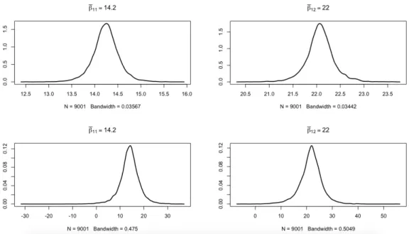
6.4 Simulation studies . . . 114
6.4.1 The case k = 2 . . . 114
6.4.2 The general case . . . 116
6.5 Parallel tempering . . . 122
6.6 Conclusion. . . 124
7 Supplementary material: Non-informative reparameterisations for location-scale mixtures 127 7.1 Spherical coordinate concept. . . 128
7.2 Data analyses . . . 132
7.2.1 Acidity data. . . 132
7.2.2 Enzyme data . . . 133
7.2.3 Darwin’s data . . . 133
7.2.4 Fishery data . . . 134
7.3 Parallel tempering algorithm . . . 135
8 Ultimixt package 139 8.1 Ultimixt . . . 139 8.2 K.MixReparametrized function . . . 141 8.3 Plot.MixReparametrized function . . . 143 8.4 SM.MAP.MixReparametrized function . . . 144 8.5 SM.MixReparametrized function . . . 146
Contents ix
9 Supplementary material: Ultimixt package 149
9.1 Description of implementation . . . 149
9.2 Application . . . 152
Chapter 1
General Introduction
1.1
Overview
In several areas of science, statistics is a powerful tool to analyze data both from con-trolled experiments such as natural sciences and from observational studies, mainly in the human sciences. Basically, a researcher expects to find methods which can provide means to judge a population from a subset of it, named a sample. Statistics has developed many different theories to be applied in different situations, and all of them have a characteristic in common and that is, given the uncertainty, they try to find the best strategy to answer scientists’ queries.
In order to apply statistics to a problem, it is a common practice to start with a population or process to be studied. When the entire population is not available and only samples are studied, the inferential statistics is needed. These inferences can take the form of testing hypotheses, estimation, regression analysis, prediction and some other technics that have been recently developed such as spatial data and data mining. Furthermore, statistical inference defines random samples and describes the population being examined by a probability distribution that may have unknown parameters. Indeed, the main purpose of statistical theories is to infer properties about the probability distribution of the population of interest us-ing observations. To do so, different paradigms of statistical inference have become established. Bayesian inference is considered as an important statistical technique especially in mathematical statistics because of its application in science beside a wide range of activities such as engineering, philosophy, medicine, sport, and law. In this thesis, we focus on the Bayesian inference. Although the original Bayesian theory was settled in the 18th century, due to various previous computational diffi-culties, only in the last 30 years, the Bayesian method has grown substantially. This growth in research and applications of Bayesian methods refers to the 1980s which mostly attributed to the discovery of Markov Chain Monte Carlo methods which removed many of the computational problems.
This thesis consists of four general parts which are briefly introduced in the following sections.
1.2
Prior distribution
The Bayesian theory deals with probability statements which are conditional on the observed value and this conditional feature introduces the main difference between Bayesian and classical inferences. Despite the differences between these statistical
methods, in many simple analysis we get superficially similar conclusions from the two approaches. A Bayesian statistical inference is based on a prior probability distribution of an uncertain quantity that expresses one’s beliefs about this quantity before some evidence is taken into account. In other words, a prior distribution is the distribution of this uncertain quantity, named parameter, before any data is observed. Once this prior distribution is set, Bayesian inference is straightforward in terms of minimizing posterior losses, computing higher posterior density or finding the predictive distribution [Robert 2001]. But in general, a prior distribution is not easy to precisely find out and most of critics of the Bayesian analysis focussed on the choice of the prior distributions. Furthermore, different perspectives are available to choose a prior while the impact of this choice on the resulting posterior inference should not be omitted even in the case it is negligible. The main point here is about the existence of a prior or the determination of an exact or even a parametrized distribution for the prior on the parameter, which is never unique.
However, the prior plays a fundamental role in drawing Bayesian inference be-cause of its exploitation combined with the probability distribution of data to yield the posterior distribution. Bayesian inference is fundamentally based on the pos-terior distribution which is used for future inference and decisions involving the parameter. [Gelman 2002] pointed out the assessment of the information that can be included in prior distributions and the properties of the resulting posterior dis-tributions, as key issues in setting a prior. He also mentioned prior distributions as the key part of Bayesian inference and classified them to three categories: Non-informative priors, highly Non-informative and moderately Non-informative hierarchical prior distributions.
In fact, the existence of fairly precise scientific or lack of information about the parameter of interest leads to two classes of priors: Informative or subjective prior, and non-informative or objective priors. One method of determining the prior is a subjective evaluation of the prior probability that can be done by using past exper-iments of the same problem that is considered as an approximation to the real prior distribution [Robert 2001]. Another methods are based on the maximum entropy de-veloped in [Jaynes 1980,Jaynes 1983] and as well as parametric approximations for priors resulting from restricting the choice of prior to a parametrized density and characterize the corresponding parameters using classical methods [Robert 2001]. Finally, other techniques such as empirical and hierarchical Bayes incorporate un-certainty about the prior distribution (for details see [Robert 2001]). All these meth-ods depend on the availability of the information on the parameter of interest. In the case of limited prior input, conjugate priors can be used to construct the prior distribution, which originated in [Raiffa 1961] and even if this choice may influence the resulting Bayesian inference, conjugate priors are not considered as part of the non-informative prior class [Robert 2001]. The most popular conjugate priors are related to the distributions associated with the exponential families which are called natural conjugate priors [Robert 2001]. This family of distributions is the only case where conjugate priors are guaranteed to exist. Despite the advantages such as being easy to deal with in both cases mathematically and computationally, the
con-1.2. Prior distribution 3 jugate priors are not away from criticism. One reason is that these distributions are overly restrictive and also they are not necessarily considered as the most robust prior distributions.
The non-informative priors are requested when no information about the pa-rameter is available. While informative priors are far from enough to allow hopes of achieving, the use of non-informative priors also underwent vary criticisms be-cause of their influences on the relative posterior distribution. Laplace’s prior is the simplest and oldest non-informative prior that is based on the principle of indiffer-ence by assigning equal probabilities to all possibilities. This prior was criticized because it results in improper resulting distributions in the case where the param-eter space is infinite. This is not always a serious problem since it may lead to proper posteriors. However, the use of improper non-informative priors may also cause problem such as the marginalization paradox shown by [Stone 1972]. Some others are the possible inadmissibility of resulting Bayes estimators, Stein’s paradox [Syversveen 1998] and in addition to the possibility of resulting improper posteriors [Kass 1996], considering equal probabilities for possible events is not coherent under partitioning as pointed out by [Robert 2001]. Another issue is the lack of invariance under the reparametrization of the parameter. The invariance of a prior is necessary when more than one inference about the parameter is needed. The best solution for obtaining invariant non-informative priors was represented by Jeffreys’ distribu-tions [Jeffreys 1939] where the information matrix of the sampling model is turned into a prior distribution. Jeffreys’ prior is most often improper which means that it does not integrate to a finite value. Another method that was initially described by [Bernardo 1979] and further developed by [Berger 1979] is the reference prior. The advantages of this method compared with Jeffreys’ method appear in the case of multidimensional problems [Syversveen 1998]. Some other methods have been also suggested by [Box 2011,Rissanen 2012,Welch 1963].
Since there is no best prior that one should use, research aims at acceding a prior so that posterior distribution is well behaved and proper while all available information about the parameter is taken into account. Recently, due to theoretical developments on sensitivity analysis, the dependence of posteriors on prior distri-butions can be checked by methods such as comparing posterior inferences under different reasonable choices of prior distribution. The first part of this thesis deals with selecting non-informative priors based on a critical review of [Seaman III 2012] and the main result of this work is to show that the Bayesian data analysis remains stable under different choices of non-informative prior distributions. A related paper was published in the journal of Applied and Computational Mathematics in July 21, 2014.
In the literature we can find a lot of theoretical and applied overviews of Bayesian statistics about the uses of non-informative priors (see [Bernardo 1994,Carlin 1996,
Gelman 2013a]). A variety of methods of driving non-informative priors have been covered by [Yang 1996]. He also listed known properties of these prior distributions. Despite the wide application of non-informative priors by Bayesian community, the handling of non-informative Bayesian testing is mostly unresolved. In the following
section, we briefly address hypotheses testing and related concepts.
1.3
Bayesian model choice
As mentioned at the beginning of this chapter, among many other types of sta-tistical inference, hypotheses testing or equivalently model selection techniques are widely applied for data analysis. Statistical hypothesis tests define a procedure of controlling the probability of incorrectly deciding that a so-called null hypothesis is false.
Differences among statistical paradigms such as frequency-based or Bayesian methods are generally much more pronounced in model checking and selection than in fitting. In a Bayesian paradigm the typical method for comparing two models involves the Bayes factors or the posterior probability of the models which are based on a specification of both likelihood and prior distribution and both are compared to-gether. Unlike standard frequency-based methods both Bayes factors and posterior probability treat the models under comparison essentially symmetrically. However, from both classical and Bayesian points of view, model selection is the problem in which we have to choose between some models on the basis of observed data but the Bayesian model comparison based on the Bayes factors does not depend on the parameters because of the integration over all parameters in each model. On the other hand, the use of Bayes factors has the advantage of automatically including a penalty for too much model structure [Kass 1995].
The literature on Bayesian model choice is considerable by now and one of the earlier, reasonably thorough reviews, appears in [Gelfand 1992]. The Bayes factors have also been the subject of much discussion in the literature in recent years and one of the comprehensive review of Bayes factors, their computation and usage in Bayesian hypothesis testing goes back to 1995 by [Kass 1995] who proposed this criterion as a solution for the comparison of models problem. However, the decision based on the Bayes factors requires a zero-one loss and [Kadane 1980] shows that these criterions are sufficient if and only if a zero-one loss obtains. Many other works on Bayesian model selection, Bayes factors and their features can be found in [Good 1950,Berger 1996].
Because of the difficulties caused by prior specification, the Bayesian approach to test hypotheses is not always straightforward especially in the case of an absolute lack of information. In fact, the use of non-informative prior distributions for testing hypotheses is delicate because of the sensitivity of Bayes factors to the choice of the prior. The typical strategy of using non-informative prior distributions with large variances clearly affects the Bayes factors [Robert 2001]. Furthermore, improper prior distributions result in improper prior predictive distributions and undefined Bayes factors. Among some other difficulties caused by Bayes factors that will be addressed in Chapter 4, a principal drawback from which both criterions, Bayes factors and posterior probability of models, suffer is that they can be difficult to compute. In all but the simplest cases, Bayes factors must be evaluated numerically
1.4. Mixture distributions 5 using methods such as importance sampling, bridge sampling and reversible jump Markov Chain Monte Carlo [Green 1995]. Another method has also been recently produced by [O’Neill 2014] for computing Bayes factors that avoids the need to use reversible jump approaches. [O’Neill 2014] show that Bayes factors for the models can be expressed in terms of the posterior means of the mixture probabilities, and thus estimated from the MCMC output. In the other hand, one solution in the case that the likelihood is not available or too costly to evaluate numerically, is the approximate Bayesian computation. Some of related works can be found in [Csilléry 2010, Toni 2010, Rattan 2013] for instance. Other proposals have been made to solve particular problems with the ordinary Bayes factor such as intrinsic Bayes factors [Berger 1996] with further modifications such as the trimmed and median variants, fractional Bayes factors [O’Hagan 1995] and posterior Bayes factors [Aitkin 1991]. Consideration of Bayes factors also leads to two of the more common criteria used for model selection such as the Bayes Information Criterion (BIC) or Schwartz’s criterion that provides a cursory first-order approximation to the Bayes factor [Robert 2001] and the Akaike Information Criterion (or AIC) [Akaike 1973]. A Bayesian alternative to both BIC and AIC based on the deviance has been developed by [Spiegelhalter 1998] which takes into account the prior information.
Because the existing solutions are not, however, universal in the second part of this thesis our focus is towards addressing the difficulties with the traditional handling of Bayesian model selection using Bayes factors by proposing a method which goes some way to removing these complications. The key idea is to consider a mixture model whose components are the competing models of interest and the traditional method for the model choice is replaced by a kind of Bayesian estimation problem that focuses on the probability weight of the mixture model. The method includes a novel strategy of reparametrizing the competing models towards common meaning parameters in all models, that allows for using the non-informative priors at least on the common parameters. Two substantial advantages of our method are the usability of the non-informative priors for Bayesian model choice and the other is that due to the standard MCMC algorithms, the Bayesian estimation of the model is straightforward and there is no need to compute the marginal likelihoods. A related paper was submitted for publication.
The third part of this thesis focuses on the parametrization of the mixture dis-tributions. In the following we briefly introduce the motivation of this work.
1.4
Mixture distributions
The earliest study about the mixture models was done by [Pearson 1894] who inves-tigated the estimation of parameters in the finite mixture model by the use of the method of moments. In 1894, [Pearson 1894] studied the dissection of asymptotic and symmetric frequency curves into two components of normal distributions. Many other papers have appeared related to the problem of statistical inference about the parameters and probabilistic properties of these densities. Since this early work,
finite mixture models have been widely used in many disciplines and there is a large body of literature on these distributions. For example in biology it is often desired to measure certain characteristics in natural populations of some particular species when the distribution of such characteristics may vary markedly with age of the individuals. Since age is difficult to ascertain in samples from populations, the biol-ogist is dealing with a mixture of distributions and the mixing in this case is done over a parameter depending on the unobservable variate, age. Some other appli-cations can be found in astronomy, ecology, genetics and so on due to the feature that they are easily applied to the data set in which two or more subpopulations are mixed together. In statistical applications, the mixture of densities can be used to approximate some parameters associated with a density.
The finite mixture models have also enjoyed intensive attentions over the re-cent years from both practical and theoretical viewpoints due to their flexibility in modeling. Some basic properties of mixtures were studied by [Robbins 1948] and [Robbins 1961] initiated the study of identifiability problem. Despite the popular-ity of mixtures, model estimation can be difficult when the number of components is unknown. In 1966, [Hasselblad 1966] first considered the estimation problem of mixtures by the method of maximum likelihood. [Rolph 1968] first considered Bayes estimation of the mixture parameters in the special case where the observations from the mixture population are restricted to the positive integers. In the framework of the Bayesian approach, one needs to assume that a prior distribution on component parameters is available. As summarized in [Frühwirth-Schnatter 2006], there are two main reasons why people may be interested in using the Bayesian method in finite mixture models. Firstly, including a suitable prior distribution or the param-eters in the framework of the Bayesian approach may avoid spurious modes when maximizing the log-likelihood function. Secondly, when the posterior distribution for the unknown parameters is available, the Bayesian method can yield valid infer-ence without relying on asymptotic normality. This is an advantage of the Bayesian method for estimating the parameters of a mixture distribution without the need of sample sizes very large. As mentioned before, the use of the conjugate prior pro-duces the posterior distribution that may belong to the tractable distribution family. However, because of the complexity of mixtures, it is impossible to find a conjugate prior for the component parameters. While the posterior distributions derived from the mixture models are non standard, MCMC methods are used to generate samples from these complex distributions [Marin 2006,Frühwirth-Schnatter 2006]. Because the main idea of Bayesian estimation using MCMC methods followed by realizing a mixture model is considered as a special case of incomplete data problem with the missing component indicator variables, the problem with conjugate priors no longer poses serious obstacles to the application of Bayesian method.
In fact, the Bayesian estimators in mixture models are always well defined as long as priors are proper. Furthermore, the unidentifiability may be resolved by well defining the parameter space or using informative priors on parameters. However, in the case where no information is available for the component parameters, the choice of the prior is more delicate. [Marin 2006] demonstrates that specifying improper
1.4. Mixture distributions 7 prior to the component parameters results in improper posterior distribution that prohibits this kind of prior to be used for mixtures. In addition, non-informative priors assigned to the parameter of a specific component can also lead to identifia-bility problems. Because if each component has its own prior parameters and few observations are allocated to this component, there will be no information at all to estimate the parameter and in the case of Gibbs sampling, the sampler gets trapped in a local mode corresponding to this component.
This problem of non-identifiability in the posterior distribution can also be due to an overfitting phenomenon. Basically this happens when some components have weights equal to zero or merged together [Frühwirth-Schnatter 2006]. A full dis-cussion about how over fitted mixtures behave can be found in [Rousseau 2011] who proved that the posterior behavior of overfitted mixtures generally depends on both the choice of the prior on the weights and the number of free parameters. [van Havre 2015] treated the issues such as non-identifiability due to overfitting, la-bel switching and also the problem of lack of mixing caused by applying standard MCMC sampling techniques when the posterior contains multiple well separated modes.
Given the difficulty with non-informative priors, one solution is to use proper pri-ors with the prior parameters chosen such that the prior is suitably weakly informa-tive priors [Richardson 1997]. This method is not always applicable because of the problem of multiple prior specifications. Another method proposed by [Diebolt 1994] is to use an improper prior under the condition of forcing each component to always have a minimal number of data points assigned to it. A related work has been re-cently developed by [Stoneking 2014] which does not result in any data dependence of the priors.
In the third part of this thesis we define a novel reparametrisation for the mix-ture of distributions based on the mean and standard deviation of the mixmix-ture itself, namely global parameters. The main feature of our method is that the non-informative prior distribution can be used on the global parameters of the mixture while the resulting posterior distribution is proper. A related paper was submitted for publication.
The reparametrized mixture model will be fitted with our R package named Ultimixt. Ultimixt provides the functionality for estimating reparametrized Gaus-sian mixture models with MCMC methods. The last part of this thesis pertains to the description of the implementation and the functions of Ultimixt. This package can accurately compute the posterior estimate of the parameters of reparametrized univariate Gaussian mixture distribution beside having the ability of graphically summarizing the posterior results.
Chapter 2
Reflecting about Selecting
Noninformative Priors
Joint work with Christian P. Robert
Abstract
Following the critical review of [Seaman III 2012], we reflect on what is presumably the most essential aspect of Bayesian statistics, namely the selection of a prior den-sity. In some cases, Bayesian inference remains fairly stable under a large range of noninformative prior distributions. However, as discussed by [Seaman III 2012], there may also be unintended consequences of a choice of a noninformative prior and, these authors consider this problem ignored in Bayesian studies. As they based their argumentation on four examples, we reassess these examples and their Bayesian processing via different prior choices. Our conclusion is to lower the de-gree of worry about the impact of the prior, exhibiting an overall stability of the posterior distributions. We thus consider that the warnings of [Seaman III 2012], while commendable, do not jeopardize the use of most noninformative priors.
Keywords: Induced prior, Logistic model, Bayesian methods, Stability, Prior distribution
2.1
Introduction
The choice of a particular prior for the Bayesian analysis of a statistical model is often seen more as an art than as a science. When the prior cannot be derived from the available information, it is generally constructed as a noninformative prior. This derivation is mostly mathematical and, even though the corresponding poste-rior distribution has to be proper and hence constitutes a correct probability density, it nonetheless leaves the door open to criticism. The focus of this note is the paper by [Seaman III 2012], where the authors consider using a particular noninformative distribution as a problem in itself, often bypassed by users of these priors: “if param-eters with diffuse proper priors are subsequently transformed, the resulting induced priors can, of course, be far from diffuse, possibly resulting in unintended influence on the posterior of the transformed parameters” (p.77). Using the inexact argument that most problems rely on MCMC methods and hence require proper priors, the authors restrict the focus to those priors.
In their critical study, [Seaman III 2012] investigate the negative side effects of some specific prior choices related with specific examples. Our note aims at
re-examining their investigation and at providing a more balanced discussion on these side effects. We first stress that a prior is considered as informative by [Seaman III 2012] “to the degree it renders some values of the quantity of inter-est more likely than others” (p.77), and with this definition, when comparing two priors, the prior that is more informative is deemed preferable. In contrast with this definition, we consider that an informative prior expresses specific, definite (prior) information about the parameter, providing quantitative information that is crucial to the estimation of a model through restrictions on the prior distribution [Robert 2007]. However, in most practical cases, a model parameter has no sub-stance per se but instead calibrates the probability law of the random phenomenon observed therein. The prior is thus a tool that summarizes the information available on this phenomenon, as well as the uncertainty within the Bayesian structure. Many discussions can be found in the literature on how appropriate choices between the prior distributions can be decided. In this case, robustness considerations also have an important role to play [Lopes 2011,Stojanovski 2011]. This point of view will be obvious in this note as, e.g., in processing a logistic model in the following section. Within the sole setting of the examples first processed in [Seaman III 2012], we do exhibit a greater stability in the posterior distributions through various noninfor-mative priors.
The plan of the note is as follows: we first provide a brief review of noninfor-mative priors in Section 4.2. In Section 2.3, we propose a Bayesian analysis of a logistic model (Seaman III et al.’s (2012) first example) by choosing the normal distribution N (0, σ2) as the regression coefficient prior. We then compare it with a g-prior, as well as flat and Jeffreys’ priors, concluding to the stability of our results. The next sections cover the second to fourth examples of [Seaman III 2012], model-ing covariance matrices, treatment effect in biomedical studies, and a multinomial distribution. When modeling covariance matrices, we compare two default priors for the standard deviations of the model coefficients. In the multinomial setting, we discuss the hyperparameters of a Dirichlet prior. Finally, we conclude with the argument that the use of noninformative priors is reasonable within a fair range and that they provide efficient Bayesian estimations when the information about the parameter is vague or very poor.
2.2
Noninformative priors
As mentioned above, when prior information is unavailable and if we stick to Bayesian analysis, we need to resort to one of the so-called noninformative priors. Since we aim at a prior with minimal impact on the final inference, we define a non-informative prior as a statistical distribution that expresses vague or general in-formation about the parameter in which we are interested. In constructive terms, the first rule for determining a noninformative prior is the principle of indiffer-ence, using uniform distributions which assign equal probabilities to all possibilities [Laplace 1820]. This distribution is however not invariant under reparametrization
2.3. Example 1: Bayesian analysis of the logistic model 11 ,(see [Berger 1980, Robert 2007] for references). If the problem does not allow for an invariance structure, Jeffreys’ priors [Jeffreys 1939], then reference priors, ex-ploit the probabilistic structure of the problem under study in a more formalized way. Other methods have been advanced, like the little-known data-translated likeli-hood of [Box 2011], maxent priors [Jaynes 2003], minimum description length priors [Rissanen 2012] and probability matching priors [Welch 1963].
[Bernardo 2009] envision noninformative priors as a mere mathematical tool, while accepting their feature of minimizing the impact of the prior selection on inference: “Put bluntly, data cannot ever speak entirely for themselves, every prior specification has some informative posterior or predictive implications and vague is itself much too vague an idea to be useful. There is no “objective" prior that represents ignorance” (p.298). There is little to object against this quote since, indeed, prior distributions can never be quantified or elicited exactly, especially when no information is available on those parameters. Hence, the concept of “true" prior is meaningless and the quantification of prior beliefs operates under uncertainty. As stressed by [Berger 1994], noninformative priors enjoy the advantage that they can be considered to provide robust solutions to relevant problems even though “the user of these priors should be concerned with robustness with respect to the class of reasonable noninformative priors” (p.59).
2.3
Example 1: Bayesian analysis of the logistic model
The first example in [Seaman III 2012] is a standard logistic regression modeling the probability of coronary heart disease as dependent on the age x by
ρ(x) = exp(α + βx)
1 + exp(α + βx). (2.1)
First we recall the original discussion in [Seaman III 2012] and then run our own analysis by selecting some normal priors as well as the g-prior, the flat prior and Jeffreys’ prior.
2.3.1 Seaman et al.’s (2012) analysis
For both parameters of the model (2.1), [Seaman III 2012] chose a normal prior N (0, σ2). A first surprising feature in this choice is to opt for an identical prior
on both intercept and slope coefficients, instead of, e.g., a g-prior (discussed in the following) that would rescale each coefficient according to the variation of the cor-responding covariate. Indeed, since x corresponds to age, the second term βx in the regression varies 50 times more than the intercept. When plotting logistic cdf’s induced by a few thousands simulations from the prior, those cumulative functions mostly end up as constant functions with the extreme values 0 and 1. This be-havior is obviously not particularly realistic since the predicted phenomenon is the occurrence of coronary heart disease. Under this minimal amount of information,
the prior is thus using the wrong scale: the simulated cdfs should have a reasonable behavior over the range (20, 100) of the covariate x. For instance, it should focus on a −5 log-odds ratio at age 20 and a +5 log-odds ratio at 100, leading to the comparison pictured in Figure 2.1 (left versus right). Furthermore, the fact that the coefficient of x may be negative also bypasses a basic item of information about the model and answers the later self-criticism in [Seaman III 2012] that the prior probability that the ED50 is negative is 0.5. Using instead a flat prior would answer the authors’ criticisms about the prior behavior, as we now demonstrate.
Figure 2.1: Logistic cdfs across a few thousand simulations from the normal prior, when us-ing the prior selected by [Seaman III 2012] (left) and the prior defined as the G-prior(right)
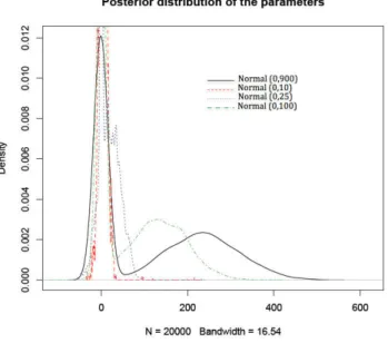
We stress that [Seaman III 2012] produce no further justification for the choice of the prior variance σ2 = 252, other than there is no information about the model parameters. This is a completely arbitrary choice of prior, arbitrariness that does have a considerable impact on the resulting inference, as already discussed. [Seaman III 2012] further criticized the chosen prior by comparing both posterior mode and posterior mean derived from the normal prior assumption with the MLE. If the MLE is the golden standard there then one may wonder about the relevance of a Bayesian analysis! When the sample size N gets large, most simple Bayesian analyses based on noninformative prior distributions give results similar to standard non-Bayesian approaches [Gelman 2013a]. For instance, we can often interpret clas-sical point estimates as exact or approximate posterior summaries based on some implicit full probability model. Therefore, as N increases, the influence of the prior on posterior inferences decreases and, when N goes to infinity, most priors lead to the same inference. However, for smaller sample sizes, it is inappropriate to
2.3. Example 1: Bayesian analysis of the logistic model 13 σ= 10 ˆ α βˆ mean s.d mean s.d 3.482 11.6554 -0.0161 0.0541 σ= 25 18.969 24.119 -0.0882 0.1127 σ= 100 137.63 64.87 -0.6404 0.3019 σ= 900 237.2 86.12 -1.106 0.401
Table 2.1: Posterior estimates of the logistic parameters using a normal prior when σ= 10, 25, 100, 900
summarize inference about the parameter by one value like the mode or the mean, especially when the posterior distribution of the parameter is more variable or even asymmetric.
The dataset used here to infer on (α, β) is the Swiss banknote benchmark (avail-able in R). The response vari(avail-able y indicates the state of the banknote, i.e. whether the bank note is genuine or counterfeit. The explanatory variable is the bill length. This data yields the maximum likelihood estimates ˜α= 233.26 and ˜β =−1.09. To check the impact of the normal prior variance, we used a random walk Metropolis-Hastings algorithm as in [Marin 2007] and derived the estimators reproduced in Table 2.1. We can spot definitive changes in the results that are caused by moves in the coefficient σ, hence concluding to the clear sensitivity of the posterior to the choice of hyperparameter σ (see also Figure 2.2).
2.3.2 Larger classes of priors
Normal priors are well-know for their lack of robustness (see e.g. [Berger 1994]) and the previous section demonstrates the long-term impact of σ. However, we can limit variations in the posteriors, using the g-priors of [Zellner 1986],
α, β | X ∼ N2(0, g(XTX)−1). (2.2)
where the prior variance-covariance matrix is a scalar multiple of the information matrix for the linear regression. This coefficient g plays a decisive role in the anal-ysis, however large values of g imply a more diffuse prior and, as shown e.g. in [Marin 2007], if the value of g is large enough, the Bayes estimate stabilizes. We will select g as equal to the sample size 200, following [Liang 2008], as it means that the amount of information about the parameter is equal to the amount of information contained in one single observation.
A second reference prior is the flat prior π(α, β) = 1. And Jeffreys’ prior constitutes our third prior as in [Marin 2007]. In the logistic case, Fisher’s in-formation matrix is I(α, β, X) = XTW X, where X = {x
Figure 2.2: Posterior distributions of the logistic parameter α when priors are N (0, σ) for σ= 10, 25, 100, 900, based on 104MCMC simulations.
W = diag{miπi(1−πi)} and mi is the binomial index for the ith count [Firth 1993].
This leads to Jeffreys’ prior {det(I(α, β, X))}12, proportional to
n � i=1 exp(α + βxi) {1 + exp(α + βxi)}2 n � i=1 x2 iexp(α + βxi) {1 + exp(α + βxi)}2 − � n � i=1 xiexp(α + βxi) {1 + exp(α + βxi)}2 �2 1 2
This is a nonstandard distribution on (α, β) but it can be easily approximated by a Metropolis-Hastings algorithm whose proposal is the normal Fisher approximation of the likelihood, as in [Marin 2007].
Bayesian estimates of the regression coefficients associated with the above three noninformative priors are summarized in Table 2.2. Those estimates vary quite moderately from one choice to the next, as well as relatively to the MLEs and to the results shown in Table 2.1when σ = 900. Figure 2.3 is even more definitive about this stability of Bayesian inferences under different noninformative prior choices.
2.4
Example 2: Modeling covariance matrices
The second choice of prior criticized by [Seaman III 2012], was proposed by [Barnard 2000] for the modeling of covariance matrices. However the paper falls short of demon-strating a clear impact of this prior modeling on posterior inference. Furthermore the adopted solution of using another proper prior resulting in a “wider" dispersion requires a prior knowledge of how wide is wide enough. We thus run Bayesian analy-ses considering prior beliefs specified by both [Seaman III 2012] and [Barnard 2000].
2.4. Example 2: Modeling covariance matrices 15 g-prior ˆ α βˆ mean s.d mean s.d 237.63 88.0377 -1.1058 0.4097 Flat prior 236.44 85.1049 -1.1003 0.3960 Jeffreys’ prior 237.24 87.0597 -1.1040 0.4051
Table 2.2: Posterior estimates of the logistic parameters under a g-prior, a flat prior and Jeffreys’ prior for the banknote benchmark. Posterior means and standard deviations remain quite similar under all priors. All point estimates are averages of MCMC samples of size 104.
Figure 2.3: Posterior distributions of the parameters of the logistic model when the prior is N (0, 9002), g-prior, flat prior and Jeffreys’ prior, respectively. The estimated posterior
distributions are based on 104MCMC iterations.
2.4.1 Setting
The multivariate regression model of [Barnard 2000] is
Yj | Xj, βj, τj ∼ N(Xjβj, τj2Inj), j = 1, 2, . . . , m. (2.3)
where Yjis a vector of njdependent variables, Xjis an nj×k matrix of covariate
vari-ables, and βj is a k-dimensional parameter vector. For this model, [Barnard 2000]
considered an iid normal distribution as the prior βj ∼ N( ¯β, Σ)
conditional on ¯β, Σ where ¯β, τj2 for j = 1, 2, . . . , m are independent and follow a normal and inverse-gamma priors, respectively. Assuming that ¯β, τ2
j’s and Σ are a
priori independent, [Barnard 2000] firstly provide a full discussion on how to choose a prior for Σ because it determines the nature of the shrinkage of the posterior of the individual βj is towards a common target. The covariance matrix Σ is defined
as a diagonal matrix with diagonal elements S, multiplied by a k × k correlation matrix R,
Σ= diag(S)Rdiag(S) .
Note that S is the k × 1 vector of standard deviations of the βjs, (S1, . . . , Sk).
[Barnard 2000] propose lognormal distributions as priors on Sj. The correlation
matrix could have (1) a joint uniform prior p(R) ∝ 1, or (2) a marginal prior obtained from the inverse-Wishart distribution for Σ which means p(R) is derived from the integral over S1, . . . , Sk of a standard inverse-Wishart distribution. In the
second case, all the marginal densities for rij are uniform when i�= j [Barnard 2000].
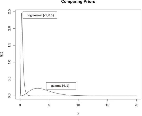
Considering the case of a single regressor, i.e. k = 2, [Seaman III 2012] chose a different prior structure, with a flat prior on the correlations and a lognormal prior with means 1 and−1, and standard deviations 1 and 0.5 on the standard deviations of the intercept and slope, respectively. Simulating from this prior, they concluded at a high concentration near zero. They then suggested that the lognormal distribution should be replaced by a gamma distribution G(4, 1) as it implies a more diffuse prior. The main question here is whether or not the induced prior is more diffuse should make us prefer gamma to lognormal as a prior for Sj, as discussed below.
2.4.2 Prior beliefs
First, Barnard et al.’s (2000) basic modeling intuition is “that each regression is a particular instance of the same type of relationship" (p.1292). This means an exchangeable prior belief on the regression parameters. As an example, they sup-pose that m regressions are similar models where each regression corresponds to a different firm in the same industry branch. Exploiting this assumption, when βj
has a normal prior like βij ∼ N( ¯βi, σi2), j = 1, 2, . . . , m, the standard deviation of
βij (Si = σi) should be small as well so “that the coefficient for the ith
explana-tory variable is similar in the different regressions" (p.1293). In other words, Si
concentrated on small values implies little variation in the ith coefficient. Toward this goal, [Barnard 2000] chose a prior concentrated close to zero for the standard deviation of the slope so that the posterior of this coefficient would be shrunken together across the regressions. Based on this basic idea and taking tight priors on Σ for βj, j = 1, . . . , m, they investigated the shrinkage of the posterior on βj as
well as the degree of similarity of the slopes. Their analysis showed that a stan-dard deviation prior that is more concentrated on small values results in substantial shrinkage in the coefficients relative to other prior choices.
Consider for instance the variation between the choices of lognormal and gamma distributions as priors of S2, standard deviation of the regression slope. Figure 2.4
2.4. Example 2: Modeling covariance matrices 17 compares the lognormal prior with mean −1 and standard deviation 0.5 and the gamma distribution G(4, 1).
Figure 2.4: Comparison of lognormal and gamma priors for the standard deviation of the regression slope.
In this case, most of the mass of the lognormal prior is concentrated on values close to zero whereas the gamma prior is more diffuse. The 10, 50, 90 percentiles of LN (−1, 0.5) and G(4, 1) are 0.19, 0.37, 0.7 and 1.74, 3.67, 6.68, respectively. Thus, choosing LN (−1, 0.5) as the prior of S2 is equivalent to believe that values of β2 in
the m regressions are much closer together than the situation where we assume S2 ∼
G(4, 1). To assess the difference between both prior choices on S2 and their impact
on the degree of similarity of the regression coefficients, we resort to a simulated example, similar to [Barnard 2000], except that m = 4 and nj = 36.
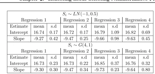
The explanatory variables are simulated standard normal variates. We also take τj ∼ IG(3, 1) and ¯β ∼ N(0, 1000I). The prior for Σ is such that π(R) ∝ 1 and we
Si ∼ LN(−1, 0.5)
Regression 1 Regression 2 Regression 3 Regression 4
Estimate mean s.d mean s.d mean s.d mean s.d
Intercept 16.74 0.17 16.72 0.17 16.79 1.09 16.82 0.69
Slope -9.27 0.42 -9.47 0.25 -9.66 0.98 -9.63 0.45
Si ∼ G(4, 1)
Regression 1 Regression 2 Regression 3 Regression 4
Estimate mean s.d mean s.d mean s.d mean s.d
Intercept 16.73 0.23 16.73 0.22 16.85 0.37 16.76 0.32
Slope -9.30 0.30 -9.47 0.34 -9.73 0.23 -9.64 0.80
Table 2.3: Posterior estimations of regression coefficients when their standard devi-ations are distributed as LN (−1, 0.5) and G(4, 1).
Si ∼ LN(−1, 0.5)
Regression 1 Regression 2 Regression 3 Regression 4
Estimate mean s.d mean s.d mean s.d mean s.d
S1 0.43 0.27 0.44 0.26 0.42 0.26 0.41 0.24
S2 0.42 0.27 0.43 0.25 0.42 0.25 0.43 0.32
Si ∼ G(4, 1)
Regression 1 Regression 2 Regression 3 Regression 4
Estimate mean s.d mean s.d mean s.d mean s.d
S1 2.31 1.28 2.33 1.29 2.29 1.29 2.29 1.26
S2 2.32 1.29 2.23 1.28 2.25 1.23 2.30 1.26
Table 2.4: Posterior estimations standard deviations of the regression coefficients when their priors are distributed as LN (−1, 0.5) versus G(4, 1).
2.4.3 Comparison of posterior outputs
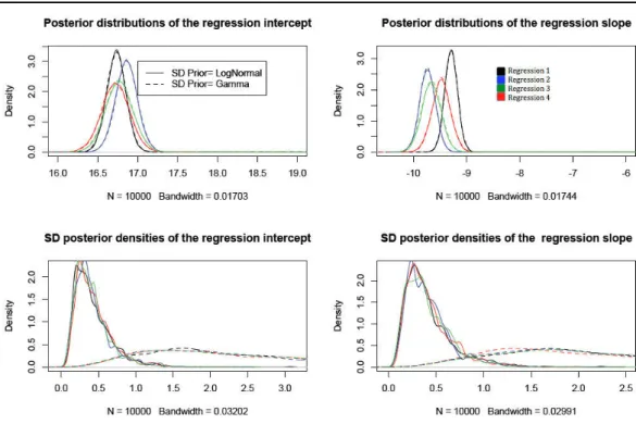
As seen in Tables 2.3and 2.4, respectively. The differences between the regression estimates are quite limited from one prior to the next, while the estimates of the standard deviations vary much more. In the lognormal case, the posterior of Si
is concentrated on smaller values relative to the gamma prior. Figure 2.5 displays the posterior distributions of those parameters. The impact of the prior choice is quite clear on the standard deviations. Therefore, since the posteriors of both intercepts and slopes for all four regressions are centered in (16.5, 17) and (−10, −9), respectively, we can conclude at the stability of Bayesian inferences on βj when
selecting two different prior distributions on Sj. That the posteriors on the Si’s
differ is in fine natural since those are hyperparameters that are poorly informed by the data, thus reflecting more the modeling choices of the experimenter.
2.5. Examples 3 and 4: Prior choices for a proportion and the
multinomial coefficients 19
Figure 2.5: Estimated posterior densities of the regression intercept (top left), slope (top right), standard deviation of the intercept (down left) and standard deviation of the slope (down right), respectively for 4 different normal regressions. All estimates based on 105
iterations simulated from Metropolis-withing-Gibbs algorithm.
2.5
Examples 3 and 4: Prior choices for a proportion
and the multinomial coefficients
This section considers more briefly the third and fourth examples of [Seaman III 2012]. The third example relates to a treatment effect analyzed by [Cowles 2002] and the fourth one covers a standard multinomial setting.
2.5.1 Proportion of treatment effect captured
In [Cowles 2002] two models are compared for surrogate endpoints, using a link function g that either includes the surrogate marker or not. The quantity of interest is a proportion of treatment effect captured: it is defined as PTE ≡ 1 − β1/βR,1,
where β1, βR,1 are the coefficients of an indicator variable for treatment in the first
and second regression models under comparison, respectively. [Seaman III 2012] restricted this proportion to the interval (0, 1) and under this assumption they pro-posed to use a generalized beta distribution on β1, βR,1 so that PTE stayed within
(0, 1).
We find this example most intriguing in that, even if PTE could be turned into a meaningful quantity (given that it depends on parameters from different models), the criticism that it may take values outside (0, 1) is rather dead-born since it suffices to impose a joint prior that ensures the ratio stays within (0, 1). This actually is
the solution eventually proposed by the authors. If we have prior beliefs about the parameter space (which depends on β1/βR,1 in this example) the prior specified
on the quantity of interest should integrate these beliefs. In the current setting, there is seemingly no prior information about (β1, βR,1) and hence imposing a prior
restriction to (0, 1) is not a logical specification. For instance, using normal priors on β1 and βR,1 lead to a Cauchy prior on β1/βR,1, which support is not limited to
(0, 1). We will not discuss this rather artificial example any further.
2.5.2 Multinomial model and evenness index
The final example in [Seaman III 2012] deals with a measure called evenness index H(θ) = −�θilog(θi)
�
log(K) that is a function of a vector θ of proportions θi,
i = 1, . . . , K. The authors assume a Dirichlet prior on θ with hyperparameters first equal to 1 then to 0.25. For the transform H(θ), Figure 2.6 shows that the first prior concentrates on (0.5, 1) whereas the second does not. Since there is nothing special about the uniform prior, re-running the evaluation with the Jeffreys prior reduces this feature, which anyway is a characteristic of the prior distribution, not of a posterior distribution that would account for the data. The authors actually propose to use the Dir(1/4, 1/4, . . . , 1/4) prior, presumably on the basis that the induced prior on the evenness is then centered close to 0.5. If we consider the more generic Dir(γ1, . . . , γK) prior, we can investigate the impact of the γi’s when
they move from 0.1 to 1. In Figure 2.6, the induced priors on H(θ) indeed show a decreasing concentration of the posterior on (0.5, 1) as γidecreases towards zero. To
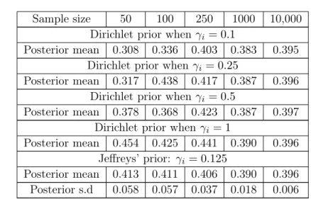
further the comparison, we generated datasets of size N = 50, 100, 250, 1000, 10, 000. Figure2.7shows the posteriors associated with each of the four Dirichlet priors for these samples, including modes that are all close to 0.4 when N = 104. Even for
moderate sample sizes like 50, the induced posteriors are almost similar. When the sample size is 50, Table 2.5 shows there is some degree of variation between the posterior means, even though, as expected, this difference vanishes when the sample size increases.
Note that, while Dirichlet distributions are conjugate priors, hence potentially lacking in robustness, Jeffreys’s prior is a special case corresponding to γi = 1/K
(here K is equal to 8). Figure 2.8reproduces the transform of Jeffreys’ prior for the evenness index (left) and the induced posterior densities for the same values of N . Since it is a special case of the above, the same features appear. A potential alter-native we did not explore is to set a non-informative prior on the hyperparameters of the Dirichlet distribution.
2.6
Conclusion
In this note, we have reassessed the examples supporting the critical review of [Seaman III 2012], mostly showing that off-the-shelf noninformative priors are not suffering from the shortcomings pointed out by those authors. Indeed, according to
2.6. Conclusion 21
Figure 2.6: Priors induced on the evenness index: Four Dirichlet prior are assigned to θ with hyperparameters all equal to 0.1, 0.25, 0.5, 1, based on 104 simulations.
Figure 2.7: Estimated posterior densities of H(θ) considering sample sizes of 50, 100, 250, 1000, 10, 000. They correspond to the priors on θ shown in Figure2.6 and are based on 104 posterior simulations. The vertical line indicates the mode of all posteriors
when sample size is large enough.
the outcomes produced therein, those noninformative priors result in stable poste-rior inferences and reasonable Bayesian estimations for the parameters at hand. We thus consider the level of criticism found in the original paper rather unfounded, as it either relies on a highly specific choice of a proper prior distribution or on bypassing basic prior information later used for criticism. The paper of [Seaman III 2012] con-cludes with recommendations for prior checks. These recommendations are mostly sensible if mainly expressing the fact that some prior information is almost always
Sample size 50 100 250 1000 10,000 Dirichlet prior when γi = 0.1
Posterior mean 0.308 0.336 0.403 0.383 0.395
Dirichlet prior when γi = 0.25
Posterior mean 0.317 0.438 0.417 0.387 0.396
Dirichlet prior when γi = 0.5
Posterior mean 0.378 0.368 0.423 0.387 0.397
Dirichlet prior when γi= 1
Posterior mean 0.454 0.425 0.441 0.390 0.396
Jeffreys’ prior: γi = 0.125
Posterior mean 0.413 0.411 0.406 0.390 0.396
Posterior s.d 0.058 0.057 0.037 0.018 0.006
Table 2.5: Posterior means of H(θ) for the priors shown in Figure 2.6 and Jeffreys’ prior on θ for sample sizes 50, 100, 250, 1000, 10, 000.
Figure 2.8: Jeffreys’ prior and estimated posterior densities of H(θ) considering sample sizes 50, 100, 250, 1000, 10, 000. The posterior distributions are based on 104posterior draws.
The vertical line indicates the mode of the posterior density when the sample size is 104.
available on some quantities of interest. Our sole point of contention is the repeated and recommended reference to MLE, if only because it implies assessing or building the prior from the data. The most specific (if related to the above) recommendation is to use conditional mean priors as exposed by [Christensen 2011]. For instance, in the first (logistic) example, this meant putting a prior on the cdfs at age 40 and age 60. The authors picked a uniform in both cases, which sounds inconsistent with the presupposed shape of the probability function.
In conclusion, we find there is nothing pathologically wrong with either the paper of [Seaman III 2012] or the use of “noninformative" priors! Looking at induced priors on more intuitive transforms of the original parameters is a commendable suggestion, provided some intuition or prior information is already available on those. Using
2.6. Conclusion 23 a collection of priors including reference or invariant priors helps as well towards building a feeling about the appropriate choice or range of priors and looking at the dataset induced by simulating from the corresponding predictive cannot hurt.
Chapter 3
Supplementary material:
Reflecting about Selecting
Noninformative Priors
This chapter contains the statistical tools, computational details and some more data analyses related to the examples studied in the chapter 2.
3.1
Example 1
The first example of Chapter2is about the Bayesian analysis of the logistic model. The non standard posterior distributions resulted by assigning different non-informative priors to the parameters of the model are given as follows
� for a flat prior π(α, β) = 1:
f (α, β|ρ, x) =exp(�n
i=1ρi(α+βxi))/�ni=1(1+exp(α+βxi))
� for g-prior α, β|X ∼ N (0, g(XTX)−1): f (α, β|ρ, x) =|XTX|1/2exp�−g/2(α β) T XTX(α β)+ �n i=1ρi(α+βxi) � /2π√g�ni=1(1+exp(α+βxi))
� and for the Jeffrey’s prior, the log-likelihood of the logistic model is given by
�(α, β) =
n
�
i=1
(ρi(α + βxi)− ln(1 + exp(α + βxi)))
The second derivate of � with respect to α and β is
∂2�(α, β) ∂α2 =− n � i=1 exp(α+βxi)/(1+exp(α+βxi))2 ∂2�(α, β) ∂β2 =− n � i=1 x2 iexp(α+βxi)/(1+exp(α+βxi))2 ∂2�(α, β) ∂α∂β =− n � i=1 xiexp(α+βxi)/(1+exp(α+βxi))2
and the matrix of Fisher information can be written as following:
I(α, β, x) = �
−�ni=1 (1+exp(α+βxexp(α+βxi)i))2 −
�n
i=1 (1+exp(α+βxxiexp(α+βxii)))2
−�ni=1 (1+exp(α+βxxiexp(α+βxii)))2 −
�n i=1 x2 iexp(α+βxi) (1+exp(α+βxi))2 �
� The invariant Jeffreys prior computed from�det(I(α, β, x)) yields the follow-ing posterior distribution for α and β
f (α, β|ρ, x) = � � � � n � i=1 exp(α + βxi) (1 + exp(α + βxi))2 n � i=1 x2i exp(α + βxi) (1 + exp(α + βxi))2 − { n � i=1 xiexp(α + βxi) (1 + exp(α + βxi))2 }2 × exp ( �n i=1ρi(α + βxi)) �n i=1(1 + exp (α + βxi)) .
We can sample from the posterior distributions above using the Metropolis-Hastings algorithm for each prior specification in which the proposal distribution is a random walk multivariate normal distribution based on the maximum likelihood estimate as starting value and the asymptotic covariance matrix of the maximum likelihood estimate as the covariance matrix of the proposal. The implementation in R can be found in [Kamary 2016a].
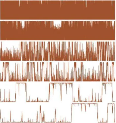
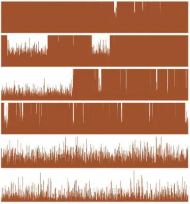
We run the Metropolis-Hastings algorithm with 104 iterations for the bank
dataset by considering the bill length as the explanatory variable, and we test three different proposal scales, τ = 0.1, 1, 5. As shown in Figures 3.1, 3.2and 3.3, for all values of τ , the chains simulated for α and β are convergent to the target distribu-tion and able to move around the normal range with decreasing autocorreladistribu-tions. However, in the case where τ = 5, the acceptance rate is low and the histograms of the output are far from the target distribution even after 104 iterations. The auto-correlation graph for τ = 1 decreases quicker than the cases where τ = 0.1, 5. By comparing the raw sequences and the autocorrelation graphs provided by three algo-rithms above and also the corresponding acceptance rates, the best mixing behavior is related to τ = 1.
By comparing the plots shown in Figures 3.1,3.2 and3.3, despite the fact that three different non informative priors were assigned to the parameters of the logistic model, there is no visible difference between the posterior draws.
3.2
Example 2
Bayesian inference of multivariate regression model 2.3 using the prior modeling defined in section 2.4derives the following joint posterior probability
3.2. Example 2 27
Figure 3.1: Simulation of posterior distribution of α and β with a multivariate normal random walk when the proposal scale τ takes values 0.1, 1, 5 and a flat prior is assigned to α and β. From top to bottom: Sequence of 104 iterations; Empirical autocorrelation;
Histogram of the last 9000 iterations compared with the target density.
Figure 3.2: Simulation of posterior distribution of α and β with a multivariate normal random walk when the proposal scale τ takes values 0.1, 1, 5 and a g-prior is assigned to α and β. From top to bottom: Sequence of 104 iterations; Empirical autocorrelation;
Histogram of the last 9000 iterations compared with the target density.
π(βj, τj2, ¯β, S, R|Yj, Xj)∝ �(βj, τj2, ¯β|Yj, Xj) × π(βj| ¯β, S, R)π(τj2)π( ¯β)π(S, R) ∝1/(τ2 j)nj/2−a−1exp � −(Yj−Xjβj)T(Yj−Xjβj)/2τ2 j �
× |diag(S)Rdiag(S)|−1/2exp�−(βj− ¯β)T(diag(S)Rdiag(S))−1(βj− ¯β)/2�
× exp(−b/τ2 j −β¯
![Figure 2.1: Logistic cdfs across a few thousand simulations from the normal prior, when us- us-ing the prior selected by [ Seaman III 2012 ] (left) and the prior defined as the G-prior(right)](https://thumb-eu.123doks.com/thumbv2/123doknet/2621180.58484/24.892.244.617.365.719/figure-logistic-thousand-simulations-normal-selected-seaman-defined.webp)