DISCUSSION PAPER SERIES
Forschungsinstitut zur Zukunft der Arbeit Institute for the Study of Labor
Home Production and Retirement in Couples:
A Panel Data Analysis
IZA DP No. 9156
June 2015 Eric Bonsang Arthur van Soest
Home Production and Retirement in
Couples: A Panel Data Analysis
Eric Bonsang
LISER and Netspar
Arthur van Soest
Tilburg University, Netspar and IZA
Discussion Paper No. 9156
June 2015
IZA P.O. Box 7240 53072 Bonn Germany Phone: +49-228-3894-0 Fax: +49-228-3894-180 E-mail: [email protected]Any opinions expressed here are those of the author(s) and not those of IZA. Research published in this series may include views on policy, but the institute itself takes no institutional policy positions. The IZA research network is committed to the IZA Guiding Principles of Research Integrity.
The Institute for the Study of Labor (IZA) in Bonn is a local and virtual international research center and a place of communication between science, politics and business. IZA is an independent nonprofit organization supported by Deutsche Post Foundation. The center is associated with the University of Bonn and offers a stimulating research environment through its international network, workshops and conferences, data service, project support, research visits and doctoral program. IZA engages in (i) original and internationally competitive research in all fields of labor economics, (ii) development of policy concepts, and (iii) dissemination of research results and concepts to the interested public. IZA Discussion Papers often represent preliminary work and are circulated to encourage discussion. Citation of such a paper should account for its provisional character. A revised version may be available directly from the author.
IZA Discussion Paper No. 9156 June 2015
ABSTRACT
Home Production and Retirement in Couples:
A Panel Data Analysis
1We analyse the effects of retirement of one partner on home production by both partners in a couple. Using longitudinal data from Germany on couples, we control for fixed household specific effects to address the concern that retirement decisions are correlated with unobserved characteristics that also affect home production. For males and females, we find that own retirement significantly increases the amounts of home production. There are negative cross-effects of retirement on home production done by the partner. The fall in household income at retirement of one of the partners is largely compensated by an increase in total household production.
JEL Classification: J22, J29, J14
Keywords: time allocation, home production, retirement, couples
Corresponding author: Arthur van Soest
Department of Econometrics & Operations Research Tilburg University P.O. Box 90153 5000 LE Tilburg The Netherlands E-mail: [email protected] 1
The authors are grateful for useful comments to Jim Been and the participants of a workshop on family economics at the Paris Graduate School of Economics 2014, the International Netspar Pension Workshop 2015 in Amsterdam, the Royal Economic Society Conference 2015 in Manchester, and a SEMILUX seminar 2015 in Luxembourg.
2
1. Introduction
Retirement is one of the main economic and social changes in the lives of most individuals and their households. Most people retire abruptly from a full-time job to a situation where they no longer take part in paid work. This not only affects their personal and household income, but also their social network and the activities on which they spend their time. For individuals in couples, retirement of the partner may have an important impact through household income, but also through the changes in the time spent by the retired partner on, for example, household production or joint leisure activities. The effects of retirement on the other partner have been used in the retirement literature to explain, for example, the stylized fact that many couples retire at almost the same point in time, in spite of an age difference (Hurd, 1990; Gustman and Steinmeier, 2000, 2009).
The economics literature has emphasized the stylized fact that household consumption expenditures drop substantially upon retirement of the main earner, known as the retirement consumption puzzle (Hamermesh, 1984; Banks et al., 1998). Several explanations for this puzzle have been given (see, e.g., Hurst, 2008, or Battistin et al., 2009), such as a reduction in work related expenses, or, the focus of this paper, a fall in required consumption expenditures to achieve a given welfare level because of an increase in time spent on household production activities. For example, Aguiar and Hurst (2005, 2007) find that after retirement, individuals in the US spend more time on shopping and preparing food, leading to a lower effective price of food consumption. Hurd and Rohwedder (2008) find that after retirement, men and women in the US spend more time on house cleaning, and men also spend more time on home improvements and gardening or yard work, probably reducing the need for expenditures on outsourcing.
Stancanelli and van Soest (2012), unlike the studies mentioned above, also consider the effect of retirement of one spouse on the time spent on home production by the partner. Using
cross-3
section data on French couples around retirement age, they find that men respond to their wives’ retirement by significantly reducing the time they allocate to home production, while there is no significant effect of men’s retirement on their wives’ hours of home production. Battistin et al. (2009) and Stancanelli and van Soest (2012) account for the potential endogeneity of retirement decisions exploiting a regression discontinuity approach, based upon the minimum age for receiving retirement benefits in Italy and France. Aguiar and Hurst (2005) also allow for endogeneity of retirement but make the stronger assumption that age can be used as an instrument for retirement. None of these studies uses panel data.
The current study uses longitudinal data on time use of German couples in the age group 45 - 75 that are followed over time from 1993 until 2009. The data set not only contains rich background information, but also has survey information on the time spent on various types of activities (housework, errands, household repairs/gardening, hobbies, education, child care), similar to the time use information in the HRS consumption and activities module (see Hurd and Rohwedder, 2008).
Previous research has shown that this type of retrospective survey information has certain drawbacks compared to the detailed diary information typically collected in specific time use surveys, but does lead to reliable results in multivariate analysis where the focus is not on the absolute amounts of time spent on certain activities but on the relations between time use and other variables (see Bonke, 2005, and Kitterød and Lyngstad, 2005). The potential drawbacks of the retrospective nature of the survey questions are in our view amply compensated by the unique longitudinal nature of the data, particularly since this allows for considering within household changes at retirement and for the use of household specific fixed effects in the empirical models. Incorporating these in the model makes it possible to identify the causal effects of retirement while controlling for time persistent confounding factors that simultaneously affect retirement and time allocation. This provides an alternative to the
4
identification strategy of Battistin et al. (2009) and Stancanelli and van Soest (2012) which is less convincing in the German institutional setting than in Italy or France because there are several standard retirement ages but not one unambiguous minimum retirement benefits eligibility age.
We analyse the effect of retirement of both partners on the time spent and the value of home production activities by both partners. We compare the results of fixed effects and random effects specifications imposing and not imposing independence between error terms and the retirement status variable. We argue that the fixed effects specification in which retirement is independent of the error terms is the preferred specification. A regression discontinuity approach where we instrument retirement of both spouses with age dummies for several institutional retirement ages in Germany gives findings of similar magnitude but much less precision.
Using the model estimates for both males and females, we find that own retirement significantly increases home production and that this increase largely compensates the income loss at retirement. We also find significantly negative cross-effects of retirement on home production done by the partner, which partly undo the effects of increases in own home production. This leads to the conclusion that retirement of one partner leads to important adjustment in home production of both partners, something that deserves more attention when trying to understand the impact of retirement on the economic and non-economic well-being of older couples.
5
2. Empirical approach
The aim of the empirical analysis is to analyse the impact of retirement of the husband and wife’s2 retirement ( m
it
R and R , respectively) on hours of home production (itf
m it
h and h ). The itf
equations to be estimated are the following:
m it m i m it f it m m it m m it R R X h 1 2 , (1) f it f i f it m it f f it f f it R R X h 1 2 , (2)
HereXit is a row vector of control variables describing personal and household characteristics of husband and wife, 1j,2j, and jare parameters to be estimated, ij represents the time-invariant unobserved heterogeneity terms and itj the time-varying error terms, for j = m, f. Assuming that itj is identically and independently distributed and independent of Xit, R , itm
and R and that itf ijis normally distributed and independent of Xit, R , and itm R , the model is itf
a standard random effects (RE) model that can be estimated with the standard estimator for linear RE models. The latter assumption may not hold if retirement (R and/or itm R ) is related itf to time-invariant unobserved heterogeneity (ij). For instance, preferences for leisure or productivity in market or non-market activities are potential drivers of both retirement and the allocation of non-working time. As a result, RE estimates of the parameters of interest are likely to be biased. The assumption of independence of explanatory variables and time-invariant heterogeneity can be relaxed using a fixed effects (FE) model and the standard (within-group) estimator for this model.
2 We also include cohabiting (heterosexual) couples but will often refer to the two partners in these couples as
6
In order to assess the validity of our results, we also estimate the model using an identification strategy similar to Stancanelli and van Soest (2012), adjusted for the German institutional setting. Following Bonsang and Klein (2012), our instruments are indicators for reaching ages 60, 63 and 65 at which individuals can start collecting retirement benefits. Which of the three ages applies depends upon the individual’s labour market history; see, for example, Börsch-Supan and Jürges (2009) for details. While reaching these specific ages has a direct effect on the probability of retirement, it is unlikely that the effect of age on home production is discontinuous at these (or other) ages, keeping retirement constant. In this case, we model retirement of both partners as probit models including the vector of control variables X and six dummies that are equal to one when the individual or the partner has reached the ages 60, 63 or 65. The three equations (for home production, own, and partner’s retirement) are then jointly estimated allowing for correlations between the three error terms using simulated maximum likelihood (See Roodman 2007, 2009). These models therefore allow for random effects (treated as part of the error terms) but not for fixed effects (since error terms are not allowed to be correlated with the exogenous explanatory variables).
3. Data
3.1 Sample
The empirical analysis uses GSOEP data from 1993 to 2009. The GSOEP is a longitudinal household survey that has started in West Germany in 1984 and in East Germany in 1990.3 We use data as of 1993 because this is the first wave where the questions about time use not only
3 The GSOEP is described in Wagner et al. (1993). It is sponsored by the Deutsche Forschungsgemeinschaft and
administered by the German Institute for Economic Research (Berlin) and the Center for Demography and Economics of Aging (Syracuse University).
7
on weekdays but also during a normal Saturday and a normal Sunday are available.4 These questions are only asked once every two years and we only use the waves in which they were asked.5 Our sample is restricted to individuals living in heterosexual couples (cohabiting or married) who are both between 45 and 75 years old and not belonging to the special subsamples of foreigners or high-income households.6 As the focus of this study is on couples’ transitions into retirement, we select couples where both partners are working when they are first observed. We drop observations where individuals report not working but are observed going back to work in later waves since we focus on retirement as definitive withdrawal from the labour market. Finally, we drop all observations with missing or unreliable values7 for the variables
used in the analysis. Our final sample includes 6,172 observations about 1,571 couples.
3.2 The measure of home production
GSOEP has survey questions on the number of hours respondents spent on several activities on a normal weekday, a normal Saturday, and a normal Sunday; see Figure 1 for the exact wording of the questions. These activities include: job, apprenticeship, and/or second job (including travel time to and from work); errands (shopping, trips to government agencies, etc); housework (washing, cooking, cleaning); child care; care and support for persons in need of care; education
4 It is important to take into account the change in time use during the weekend because some preliminary analysis
revealed that individuals tend to substitute home production during the weekend to home production during the week when they retire (results are available upon request). As a consequence, using information on time use during weekdays only would overestimate the effect of retirement on home production.
5 Moreover, the question regarding time use was slightly different before 1991. Before 1991, it did not make a
distinction between time devoted to housework (such as washing, cooking, or cleaning) and time devoted to errands (such as shopping, trips to government agencies…).
6 The special foreigner subsamples cover persons in private households with a Turkish, Greek, Yugoslavian,
Spanish or Italian household head. A subsample of high-income households has been added in 2002.
8
and further training (also school, university); repairs on and around the house, including car repairs or garden work; and hobbies and other free-time activities.
[Figure 1 about here]
Following Schwerdt (2005) and Frazis and Stewart (2011), our measure of home production includes errands, housework, and repairs on and around the house, including car repairs or garden work. We exclude care and support in need of care because it is mainly related to care provided to non-household members and thus should not be taken into account as an input in the home production of the household. We also exclude child care as it is mostly related to time spent with grandchildren and is thus plausibly not an input in the home production function. Anyway, including these time use categories or not should not matter much as they only represent a small fraction of the total time for the respondents in the sample we have selected. One may also question the inclusion of repairs on and around the house (including gardening), as it may be considered as a leisure activity rather than a productive activity. We will assess the robustness of our results by using a more conservative measure of home production excluding this activity from home production.
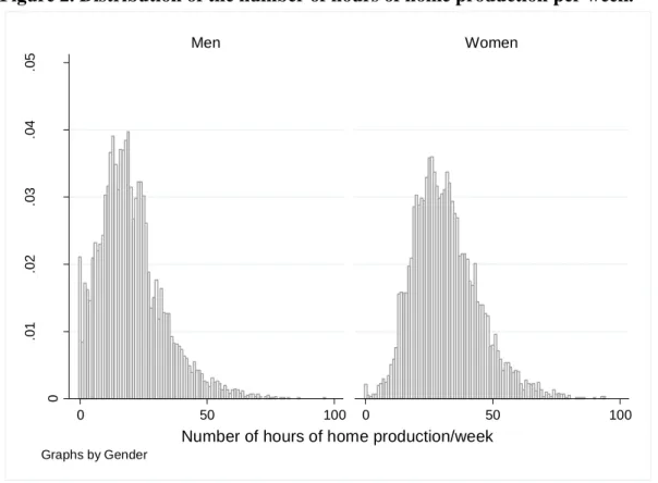
In order to construct a measure of home production done per week, we add the reported home production on a normal Saturday and a normal Sunday to the reported home production on a normal weekday multiplied by five. Figure 2 presents the distribution of the time spent on home production per week for men and women in our estimation sample. We observe that women spend more time on home production than men do and that there are barely any women reporting zero hours of home production. Not spending any time on home production is a bit more common among men, but still uncommon (about 2 percent). Given the low proportion of individuals reporting zero hours of home production, the use of censored regression (tobit) models instead of linear models will hardly affect the results.
9
[Figure 2 about here]
3.3 Retirement
There are many definitions of retirement. For the purpose of our analysis, we follow Lazear (1986) and define an individual as retired if he or she is definitively out of the labour force with the intention of staying out permanently. As in Bonsang, Adam and Perelman (2012), Bonsang and Klein (2012), Coe and Zamarro (2011), Mazzonna and Peracchi (2012), and Rohwedder and Willis (2010), individuals are defined as “Working” if they report to be currently working for pay and “Retired” if they report not working. One issue with this definition is that we may classify some individuals as retired although they are actually unemployed. Given that we drop observations for individuals who are not working but go back to work in later waves, the unemployed individuals in our sample never succeed in finding a new job and can be classified as involuntary retired, following the definition of Bonsang and Klein (2012).8
[Figure 3 about here]
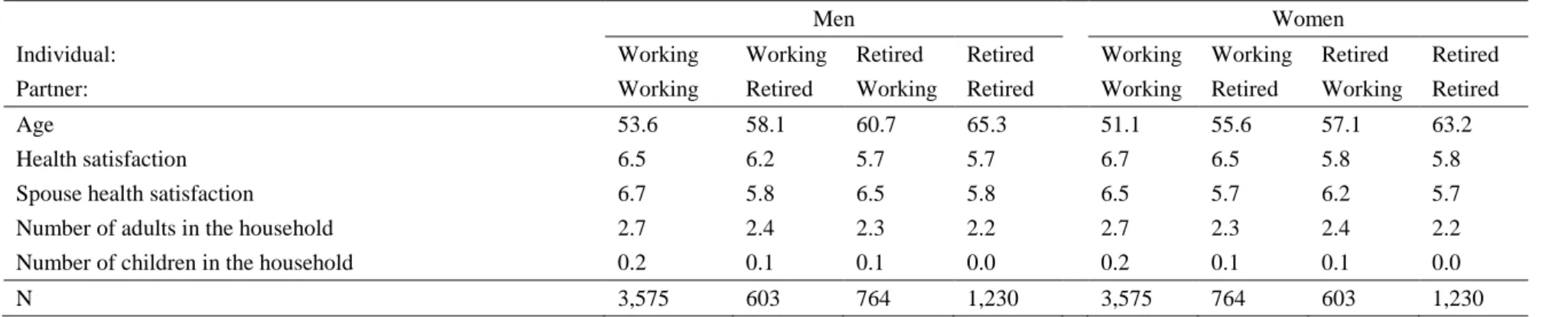
3.4. Control variables
We use household characteristics and health indicators as additional explanatory variables to control for time varying factors that are likely to be related to both home production and retirement. We control for age by including a third-order polynomial in age of the individual and the age of the partner (age of the partner is not included in fixed effects models due to collinearity with age of the respondent). Household characteristics consist of the numbers of adults and children in the household. We also include a measure of self-assessed general health
8 The distinction between “involuntarily retired” and “unemployed” individuals depends on how long we can
follow individuals after they have stopped working. We do not expect this to be a severe problem because we observe most individuals for at least some years after they stop working.
10
for each partner in the models, based on the question “How satisfied are you with your health?” where respondents can answer on a Likert scale from 0 (not satisfied at all) to 10 (very satisfied). Table 1 presents the means of the control variables for men and women by retirement status of both partners.
[Table 1 about here]
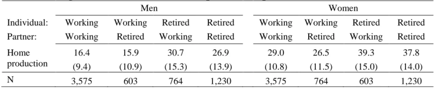
4. Descriptive statistics
Table 2 shows the average number of hours of home production by gender and retirement status of both partners. In dual earner couples, men on average spend about 16 hours per week on home production compared to 29 hours for women. An average retired man spends 30 hours on home production if his partner is working and 27 hours if she is retired. For retired women, there is no significant difference in average hours of home production depending on the labour force status of her partner. Working women on the other hand spend less time on home production when their partner is retired (29 versus 26.5 hours).
[Table 2 about here]
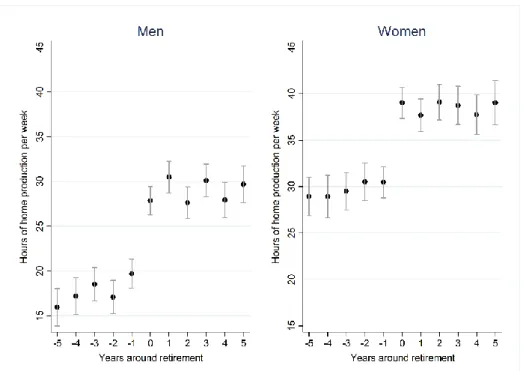
The longitudinal dimension of the survey allows us to observe the evolution of home production around the age of retirement of each partner. Figures 4 and 5 present average hours of home production per week in the five years before and the five years after own retirement (Figure 4) and retirement of the partner (Figure 5). In Figure 4, we observe a significant increase in home production in the year of own retirement for both men and women. In the years before retirement, home production increases slightly, much less than the substantial change in the year of retirement. In the years after retirement, there does not seem to be any specific trend, suggesting that dynamics involving lagged adjustment to retirement status does not play an
11
important role. The increase is similar in magnitude for men and women (although the levels of home production are always much higher for women).
[Figures 4 and 5 about here]
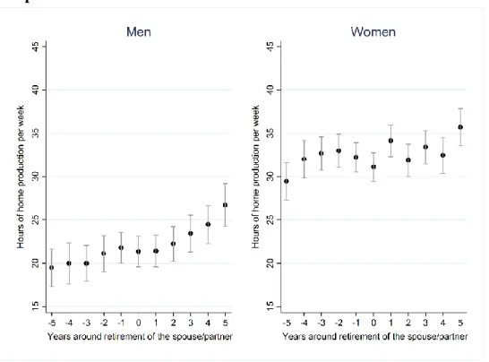
Figure 5 shows no significant change in home production around the retirement age of the partner, for both men and women, suggesting that there is no cross-effect of retirement on home production of the partner. We have to keep in mind, however, that these figures are only descriptive, not controlling for other determinants of home production (such as own labour force status). The empirical analysis below will overcome this limitation.
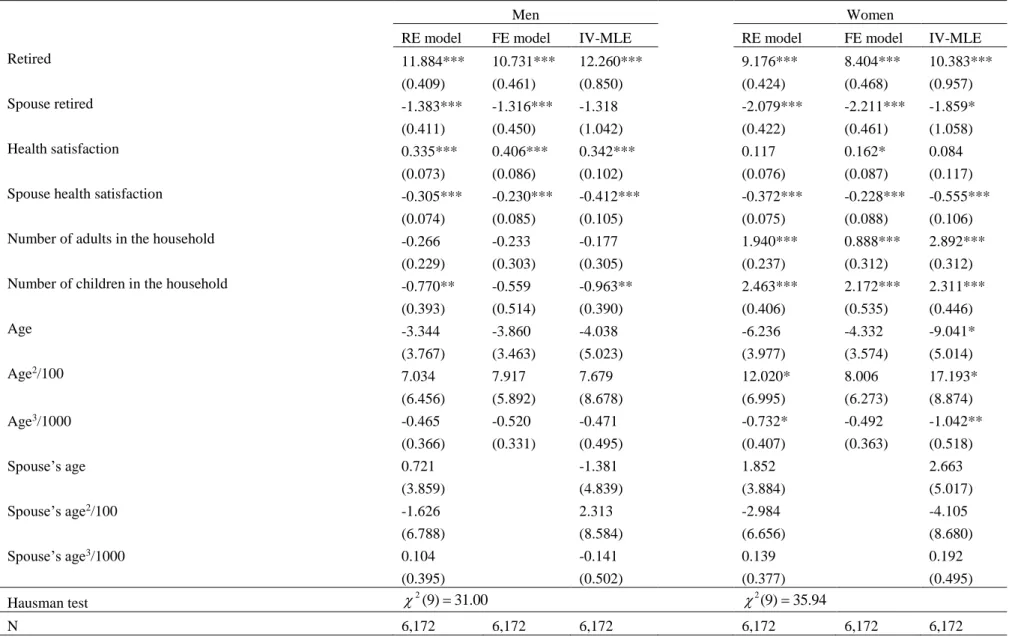
5. Results
Table 3 presents the results of the effects of own and spouse’s retirement on time devoted to home production for men and women. We present the results of the standard random-effects model, the standard fixed effects model, and the model allowing for correlation between the error term of the home production equation and the retirement equation of each partner. The results are qualitatively quite similar across all these models. Still, for both men and women, a Hausman test rejects the hypothesis that individual unobserved effects and the explanatory variables are uncorrelated. In other words, the fixed effects model is preferred to the random effects specification. The estimated effect of retirement on home production is slightly lower in the fixed effects model than for the random effects model. For men, retirement increases the number of hours devoted to home production by approximately 11 hours per week. For women, we observe a lower effect of retirement than for men (about 8 hours per week). Table 3 also highlights significantly negative cross-effects of retirement on home production of the partner.
12
The partner’s retirement decreases the time devoted to home production by about 1 hour per week for men and by about 2 hours for women.9
[Table 3 about here]
While exhibiting larger standard errors, the point estimates of the instrumental variable models are very close to those from the fixed effects model, suggesting that endogeneity due to reverse causality or time-variant unobserved confounding factors are not driving our main results.10 We therefore conclude that the fixed effects model is the preferred specification.
Our estimated effects of retirement on home production are remarkably similar in magnitude to those obtained by Van Soest and Stancanelli (2012) who found that, at retirement, own home production increases by about 11.3 hours per week for men and 8.8 hours for women in France. However, our estimated effects of partner’s retirement on own home production differ from those of Van Soest and Stancanelli (2012). They identified a large effect of partner’s retirement on home production of men (home production of French men decreases by 8.6 hours per week when their partner retires) but no effect for women. While we found significant cross-effects for men as well as women, the magnitudes of these effects are modest compared to the direct
9 We have also estimated models in which the retirement dummies are replaced by the number of hours of paid
work. Results are presented in Table A1 in the Appendix. It is worth noting that the estimated coefficients for the number of hours of paid work of the individual and for the number of hours of paid work of the spouse are similar for men and women, contrary to the estimated coefficients for the retirement dummies in Table 3. It suggests that the lower effect of own retirement on home production for women is explained by the fact that working women spend on average less hours of paid work per week than men. In our sample, working men spend on average 48 hours of paid work per week compared to 36 hours for women.
10 The full results of the Instrumental Variables are presented in Table A2 and A3 in the Appendix. The first-stage
equations show that our instruments are relevant for predicting retirement: the age-specific dummies (the instruments) are all significant in the retirement model for men and the dummies for reaching 60 years of age is highly significant for women. Table A4 shows the results of the model when all four equations are estimated simultaneously.
13
effect of retirement on own home production of each partner. As a result, total home production of couples still increases when both partners retire even when taking the cross-effects into account. This is different from the result for France in Van Soest and Stancanelli (2012), where total home production increases for men but the negative cross-effect annihilates the positive direct effect of retirement on home production for women.
These results clearly show that ignoring the effect of retirement on partner’s home production will result in biased estimates of the effect of retirement of couples on home production. First of all, the direct effect of retirement on home production in a model where partner’s retirement is omitted will result in an under-estimation of the direct effect of retirement on home production (as long as own retirement and partner’s retirement are positively correlated and partner’s retirement is negatively correlated with own home production). Note however that this bias is negligible in our case: if we omit partner’s retirement status from the fixed effects model, the estimated direct effect of retirement is 10.560 (Standard error: 0.457) for men and 8.106 (Standard error: 0.465) for women. Second and more importantly, the estimated effect of retirement of both partners on total home production would be over-estimated by about 20 percent by ignoring the cross-effects.
Some other results regarding the other explanatory variables are worth mentioning. For men, better own health is associated with a higher level of home production, but partner’s health has the opposite sign. Surprisingly, own health is not related to home production for women. However, like for men, better health of the spouse reduces own time spent on home production. There are also noticeable differences between men and women in the way their home production changes with household composition. While (in the fixed effects model), the numbers of adults and children in the household are unrelated to home production of men, they are positively related to home production of women.
14
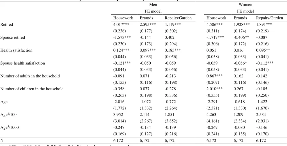
Table 4 presents the results of the fixed effects model for each component of home production separately (housework, errands, and repairs/gardening).11 Men increase time devoted to housework by about 4.02 hours per week, compared to 4.59 hours for women. Time devoted to errands increases by 2.59 hours per week for men and 1.93 hours for women. The increase in repairs/gardening is larger for men than for women (4.12 versus 1.82). More importantly, the results show that the main source of the negative cross-effect of retirement on total home production comes from the negative effect on housework. For both men and women, about 40% of the increase in housework due to own retirement is annihilated once the partner retires.
[Table 4 about here]
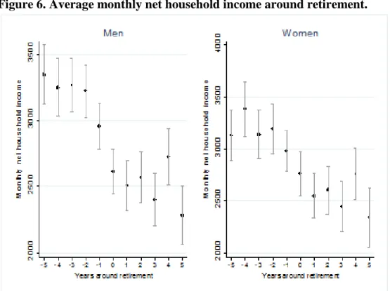
6. Does home production compensate for the income loss due to retirement?
The fundamental question in relation to the retirement-consumption puzzle is whether home production is able to compensate the income loss due to retirement. Figure 6 presents the evolution of monthly net household income around retirement of men and women. As expected, we observe a drop in income once the individual retires from the labour force. For male retirement the drop is substantial: from about 3,250 Euros per month two years before retirement to about 2,500 Euros after retirement. We observe a similar pattern for retirement of women but the size of the drop is smaller.
[Figure 6 about here]
The challenge is to estimate the value of home production. There exist different ways to estimate this and each method has its advantages and drawbacks. Following Frazis and Steward (2011) and Frick et al. (2012), we decided value home production using the replacement cost
15
approach (and not the opportunity cost approach), which defines the value of the time spent on home production as the cost of purchasing home production services in the market. This method uses either the generalist or the specialist wage approach. For this paper, we decided to use the simple and transparent method of imputing a value of home production with a uniform imputed wage for home production. Following Frick et al. (2012), we impute a net hourly wage of 4 Euros to approximate the wage of informal employment in the private sector, or a wage of 8.50 Euros of 2014 that approximates the minimum wage that has recently been approved by the German Parliament. As our data cover a relatively long period, we adjust those amounts for inflation by adjusting the amounts to 2009 prices. We then compute the total resources of the household as its net monthly household income plus the amount of time spent on home production per month by the couple, multiplied with the imputed wage rate (either 4 or 8.5 Euros/hour).
Table 5 presents the results of fixed effects models, similar to the fixed effects model of hours of home production in the previous section, but with the log of total resources of the household as the dependent variable. Three assumptions are made: no value for home production, home production valued at 4 Euros per hour, and home production valued at 8.5 Euros per hour. The results help us to quantify to which extent home production is able to cover for the income loss due to retirement.
[Table 5 about here]
The difference between the first column and the other columns shows that taking account of home production has a remarkably important effect on the loss of resources due to retirement of the couple. While household income drops by 14 percent when the man retires and 10 percent when the woman retires (first column), the drop in total resources of the household is only 5
16
percent for the man’s retirement and 3 percent for the woman’s retirement when we impute the most conservative value to home production (4 Euros per hour). If we use the minimum wage of 8.5 Euros per hour to value home production, the drop completely disappears for both partners’ retirement (final column). The valorisation of home production has a bigger tempering effect on the drop of resources due to the retirement of men than for women because, as seen in Table 3, home production of men increases more at retirement than for women and also because the negative spillover effect is larger for women than for men.
Using the narrower definition of home production by excluding repairs/gardening (See Section 3) provides similar results. The drop in total resources of the household is 8 percent for men’s retirement and 5 percent for women’s retirement when we impute the most conservative value to home production. If we use the minimum wage of 8.5 Euros per hour to value home production, the drop in resources remains statistically significant for both partners’ retirement, but the size is relatively small: resources fall by 4% when the man retires and by 1.5% when it is the woman who retires.12
7. Concluding remarks
In this paper we have analysed the effect of retirement of couples on home production of both partners. We have used longitudinal German data from 1993 to 2009 with information on the time spent on several types of home production activities, and models taking account of the endogeneity of retirement in a model of home production. We have shown that fixed effects models provide results that are similar to the results using instrumental variable models in the spirit of Van Soest and Stancanelli (2012). Own retirement substantially increases the time devoted to home production for both men and women. Furthermore, we have identified
12 See Table A7 in Appendix. Table A6 shows the results of the models used for the results obtained in Table 3
17
significant spillover effects of retirement on home production by the partner: Both men and women decrease the time spent on home production when their partner retires from the labour force: Not taking into account those spillover effects results in an over-estimation of the effect of retirement of the couple on home production by about 20 percent.
Since the data provide information on the time spent on home production activities but not the value of home produced goods, the value per hour had to be imputed. Imputing the value of each hour of home production in several ways, we have shown that, accounting for the spill-over effects on the other partner, changes in home production largely compensate for the loss of financial resources of the household when its members retire from the labour force. This paper therefore contributes to the literature on the retirement-consumption puzzle, lending support to the fact that taking home production of couples into account makes the retirement-consumption puzzle much less of a puzzle, even when accounting for the opposite effects on the two partners in a couple.
Our study is not without limitations. First, our measure of home production is based on use measured with recall survey questions. This kind of measure has been criticized in the time-use literature. On the other hand, the main advantage of our measure is that it is available for a large and long panel, something which is crucially not the case for the typical time use data based upon diaries. A large effort in collecting longitudinal data based on diary data would be needed in order to investigate whether diary data would really make a difference, not only for the estimated levels of home production but also for the estimated changes in home production due to retirement.
18
References
Aguiar, Mark, and Eric Hurst. 2005. Consumption versus expenditure. Journal of Political Economy, 113(5): 919-948.
Aguiar, Mark, and Eric Hurst. 2007. Life-cycle prices and production. American Economic Review, 97(5): 1533-1559.
Banks, James, Richard Blundell and Sarah Tanner (1998), Is there a retirement savings puzzle? American Economic Review, 88(4), 769-788.
Battistin, Erich, Agar Brugiavini, Enrico Rettore and Guglielmo Weber. 2009. The retirement consumption puzzle: Evidence from a regression discontinuity approach. American Economic Review, 99(5): 2209-2226.
Bonke, Jens. 2005. Paid work and unpaid work: Diary information versus questionnaire information. Social Indicators Research, 70: 349-368.
Bonsang, Eric, Stéphane Adam, and Sergio Perelman. 2012. Does retirement affect cognitive functioning? Journal of Health Economics, 31(3): 490-501.
Bonsang, Eric, and Tobias Klein. 2012. Retirement and subjective well-being. Journal of Economic Behavior and Organization, 83(3): 311-329.
Börsch-Supan, Axel, and Hendrik Jürges. 2009. Early retirement, social security and well-being in Germany. in: David Wise (ed.), Developments in the Economics of Aging, 173-199. The University of Chicago Press, Chicago.
Coe, Norma B., and Gema Zamarro. 2008. Retirement Effects on Health in Europe. Journal of Health Economics, 30(1): 77-86.
Frazis, Harley, and Jay Stewart. 2011. How Does Household Production Affect Measured Income Inequality? Journal of Population Economics, 24 (1): 3-22.
Frick, Joachim R., Markus M. Grabka and Olaf Groh-Samberg. 2012. The impact of home production on economic inequality in Germany. Empirical Economics, 43: 1143-1169. Gustman, Alan L., and Thomas L. Steinmeier. 2000. Retirement in dual-career families: A
structural model. Journal of Labor Economics, 18: 503-545.
Gustman, Alan L. and Thomas L. Steinmeier. 2009, Integrating retirement models. NBER Working Paper 15607.
Hamermesh, Daniel S. 1984. Consumption during retirement: The missing link in the life-cycle. Review of Economics and Statistics, 66(1): 1-7.
Hurd, Michael A. 1990. The joint retirement decision of husbands and wives, in: Issues in the Economics of Aging, ed. David A. Wise, 231-258. Cambridge MA: NBER.
19
Hurd, Michael A., and Susann Rohwedder. 2008. The retirement consumption puzzle: Actual spending change in panel data. NBER Working Paper 13929.
Hurst, Eric. 2008. The retirement of a consumption puzzle. NBER Working Paper 13789. Kitterød, Ragni H., and Torkild H. Lyngstand. 2005. Diary versus questionnaire information
on time spent on housework – The case of Norway. International Journal of Time Use Research, 2(1): 13-32.
Lazear, Edward P. 1986. Retirement from the Labor Force. In Handbook of Labor Economics, Vol. 1, ed. Orley Ashenfelter and Richard Layard, 305-55. London: Elsevier.
Mazzonna, Fabrizio, and Franco Peracchi, 2012. Aging, cognitive abilities, and retirement. European Economic Review, 56(4): 691-710.
Rohwedder, Susann and Robert J. Willis. 2010. Mental Retirement. Journal of Economic Perspectives, 24(1): 1-20.
Roodman, David. 2007. CMP: Stata Module to Implement Conditional (Recursive) Mixed Process Estimator. Boston College Department of Economics Statistical Software Component S456882.
Roodman, David. 2009. Estimating Fully Observed Recursive Mixed-Process Models with CMP. Center for Global Development Working Paper 168.
Schwerdt, Guido. 2005. Why does consumption fall at retirement? Evidence from Germany. Economic Letters, 89(3): 300-305.
Stancanelli, Elena, and Arthur van Soest. 2012. Retirement and home production: A regression discontinuity approach. American Economic Review, 102(3): 600-605.
Wagner, Gert, Richard V. Burkhauser, and Frederike Behringer 1993. The English language public use file of the German Socio-Economic Panel Study, Journal of Human Resources, 28(2), 429-433.
20
21
Figure 2. Distribution of the number of hours of home production per week.
0 .0 1 .0 2 .0 3 .0 4 .0 5 0 50 100 0 50 100 Men Women D e n s it y
Number of hours of home production/week Graphs by Gender
22
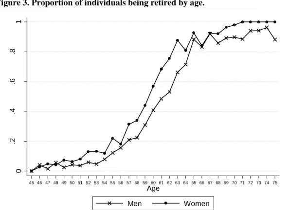
Figure 3. Proportion of individuals being retired by age.
0 .2 .4 .6 .8 1 P ro p o rt io n o f in d iv id u a ls r e ti re d 45 46 47 48 49 50 51 52 53 54 55 56 57 58 59 60 61 62 63 64 65 66 67 68 69 70 71 72 73 74 75 Age Men Women
23
Figure 4. Average number of hours of home production per week around own retirement
Note: The dots represent the average number of hours of home production per week and the vertical lines represent the 95% confidence interval.
24
Figure 5. Average number of hours of home production per week around retirement of the spouse.
Note: The dots represent the average number of hours of home production per week and the vertical lines represent the 95% confidence interval.
25
Figure 6. Average monthly net household income around retirement.
Note: The dots represent the average monthly net household income and the vertical lines represent the 95% confidence interval.
26
Table 1. Means of explanatory variables.
Men Women
Individual: Working Working Retired Retired Working Working Retired Retired
Partner: Working Retired Working Retired Working Retired Working Retired
Age 53.6 58.1 60.7 65.3 51.1 55.6 57.1 63.2
Health satisfaction 6.5 6.2 5.7 5.7 6.7 6.5 5.8 5.8
Spouse health satisfaction 6.7 5.8 6.5 5.8 6.5 5.7 6.2 5.7
Number of adults in the household 2.7 2.4 2.3 2.2 2.7 2.3 2.4 2.2
Number of children in the household 0.2 0.1 0.1 0.0 0.2 0.1 0.1 0.0
27
Table 2. Average number of hours of home production per week.
Men Women
Individual: Working Working Retired Retired Working Working Retired Retired Partner: Working Retired Working Retired Working Retired Working Retired Home
production
16.4 15.9 30.7 26.9 29.0 26.5 39.3 37.8
(9.4) (10.9) (15.3) (13.9) (10.8) (11.5) (15.0) (14.0)
N 3,575 603 764 1,230 3,575 764 603 1,230
28
Table 3. Retirement and hours of home production per week in couples: Linear models
Men Women
RE model FE model IV-MLE RE model FE model IV-MLE
Retired 11.884*** 10.731*** 12.260*** 9.176*** 8.404*** 10.383*** (0.409) (0.461) (0.850) (0.424) (0.468) (0.957) Spouse retired -1.383*** -1.316*** -1.318 -2.079*** -2.211*** -1.859* (0.411) (0.450) (1.042) (0.422) (0.461) (1.058) Health satisfaction 0.335*** 0.406*** 0.342*** 0.117 0.162* 0.084 (0.073) (0.086) (0.102) (0.076) (0.087) (0.117)
Spouse health satisfaction -0.305*** -0.230*** -0.412*** -0.372*** -0.228*** -0.555***
(0.074) (0.085) (0.105) (0.075) (0.088) (0.106)
Number of adults in the household -0.266 -0.233 -0.177 1.940*** 0.888*** 2.892***
(0.229) (0.303) (0.305) (0.237) (0.312) (0.312)
Number of children in the household -0.770** -0.559 -0.963** 2.463*** 2.172*** 2.311***
(0.393) (0.514) (0.390) (0.406) (0.535) (0.446) Age -3.344 -3.860 -4.038 -6.236 -4.332 -9.041* (3.767) (3.463) (5.023) (3.977) (3.574) (5.014) Age2/100 7.034 7.917 7.679 12.020* 8.006 17.193* (6.456) (5.892) (8.678) (6.995) (6.273) (8.874) Age3/1000 -0.465 -0.520 -0.471 -0.732* -0.492 -1.042** (0.366) (0.331) (0.495) (0.407) (0.363) (0.518) Spouse’s age 0.721 -1.381 1.852 2.663 (3.859) (4.839) (3.884) (5.017) Spouse’s age2/100 -1.626 2.313 -2.984 -4.105 (6.788) (8.584) (6.656) (8.680) Spouse’s age3/1000 0.104 -0.141 0.139 0.192 (0.395) (0.502) (0.377) (0.495) Hausman test 2(9)31.00 2(9)35.94 N 6,172 6,172 6,172 6,172 6,172 6,172
Note: IV-MLE are the maximum likelihood estimates where the home production equation is specified as a linear model and retirement equations are specified as probits. The standard errors (in parentheses) are clustered at the individual level. *** p<0.01, ** p<0.05, * p<0.1
29
Table 4. Retirement and hours of components of home production per week in couples: Fixed effects linear models
Men Women
FE model FE model
Housework Errands Repairs/Garden Housework Errands Repairs/Garden
Retired 4.017*** 2.595*** 4.119*** 4.586*** 1.928*** 1.891*** (0.236) (0.177) (0.302) (0.311) (0.174) (0.219) Spouse retired -1.573*** -0.144 0.402 -1.717*** -0.406** -0.087 (0.230) (0.173) (0.294) (0.306) (0.172) (0.216) Health satisfaction 0.124*** 0.097*** 0.185*** 0.051 0.016 0.095** (0.044) (0.033) (0.056) (0.058) (0.033) (0.041)
Spouse health satisfaction -0.121*** -0.050 -0.059 -0.059 -0.056* -0.112***
(0.044) (0.033) (0.056) (0.058) (0.033) (0.041)
Number of adults in the household -0.091 0.071 -0.213 0.867*** 0.162 -0.142
(0.155) (0.116) (0.198) (0.207) (0.116) (0.146)
Number of children in the household -0.358 0.077 -0.278 2.010*** 0.267 -0.105
(0.263) (0.198) (0.336) (0.355) (0.199) (0.250) Age -2.016 -1.072 -0.772 -2.291 -0.618 -1.422 (1.772) (1.332) (2.264) (2.371) (1.330) (1.670) Age2/100 3.952 2.114 1.851 4.263 1.209 2.534 (3.014) (2.267) (3.852) (4.161) (2.334) (2.931) Age3/1000 -0.247 -0.134 -0.139 -0.267 -0.080 -0.146 (0.169) (0.127) (0.216) (0.241) (0.135) (0.170) N 6,172 6,172 6,172 6,172 6,172 6,172
30
Table 5. Retirement and ln(monthly household resources): Fixed effects models Fixed effects model
No home production Home production valued at 4/hour Home production valued at 8.50/hour Man retired -0.139*** -0.054*** -0.008 (0.012) (0.009) (0.009) Woman retired -0.101*** -0.031*** 0.007 (0.012) (0.009) (0.009)
Man’s health satisfaction 0.003 0.003* 0.003*
(0.002) (0.002) (0.002)
Woman’s health satisfaction 0.006*** 0.005*** 0.004**
(0.002) (0.002) (0.002) Number of adults in the household 0.146*** 0.110*** 0.090*** (0.008) (0.006) (0.006) Number of children in the household 0.096*** 0.072*** 0.060*** (0.013) (0.011) (0.010) Man’s age 0.122 0.117* 0.089 (0.088) (0.071) (0.069) Man’s age2/100 -0.192 -0.180 -0.132 (0.150) (0.120) (0.117) Man’s age3/1000 0.010 0.009 0.006 (0.008) (0.007) (0.007) N 5,660 5,660 5,660 *** p<0.01, ** p<0.05, * p<0.1 Standard errors in parentheses.
31
APPENDIX (not intended for publication).
Table A1. Hours of work and hours of home production per week in couples: Linear models
Men Women
RE model FE model IV-MLE RE model FE model IV-MLE
Hours of work/week -0.264*** -0.242*** -0.195* -0.270*** -0.259*** -0.112
(0.008) (0.009) (0.118) (0.009) (0.010) (0.124)
Spouse’s hours of work/week 0.070*** 0.049*** 0.059 0.045*** 0.050*** 0.091
(0.009) (0.010) (0.128) (0.008) (0.009) (0.110)
Health satisfaction 0.376*** 0.430*** 0.314* 0.123* 0.207** -0.050
(0.071) (0.084) (0.179) (0.074) (0.085) (0.150)
Spouse health satisfaction -0.342*** -0.242*** -0.457*** -0.399*** -0.230*** -0.634***
(0.072) (0.084) (0.142) (0.073) (0.085) (0.176)
Number of adults in the household -0.066 -0.186 -0.016 1.570*** 0.701** 2.610***
(0.222) (0.296) (0.536) (0.228) (0.304) (0.513)
Number of children in the household -0.431 -0.462 -0.652 1.127*** 1.226** 1.763**
(0.383) (0.505) (0.865) (0.394) (0.522) (0.837) Age 0.990 0.728 -7.047 -1.568 0.616 -18.937** (3.681) (3.412) (10.938) (3.856) (3.497) (8.639) Age2/100 -0.719 -0.196 12.583 3.421 -0.983 34.142** (6.311) (5.809) (18.764) (6.786) (6.143) (15.272) Age3/1000 -0.022 -0.056 -0.730 -0.221 0.036 -1.973** (0.358) (0.327) (1.042) (0.395) (0.356) (0.872) Spouse’s age -0.244 -3.001 1.290 -4.416 (3.767) (8.825) (3.769) (10.496) Spouse’s age2/100 0.229 5.271 -2.008 8.079 (6.630) (15.608) (6.461) (18.012) Spouse’s age3/1000 -0.003 -0.308 0.085 -0.487 (0.386) (0.891) (0.366) (1.001) Hausman test 2(9)39.00 2(9)23.62 N 6,172 6,172 6,172 6,172 6,172 6,172
Note: IV-MLE are the maximum likelihood estimates where the home production equations and the hours of work equations are specified as linear models. The standard errors (in parentheses) are clustered at the individual level. *** p<0.01, ** p<0.05, * p<0.1
32
Table A2. Retirement and hours of home production per week: Full results of the linear IV-MLE model. Men
Retired Spouse retired Home production Retired 12.260*** (0.850) Spouse retired -1.318 (1.042) 1[Age>=60] 0.189** 0.025 (0.082) (0.088) 1[Age>=63] 0.214*** 0.118 (0.080) (0.081) 1[Age>=65] 0.300*** -0.083 (0.099) (0.098) 1[Spouse’s Age>=60] 0.033 0.413*** (0.088) (0.083) 1[Spouse’s Age>=63] 0.078 0.173* (0.106) (0.100) 1[Spouse’s Age>=65] -0.197 -0.123 (0.126) (0.127) Health satisfaction -0.107*** -0.001 0.342*** (0.015) (0.013) (0.102)
Spouse health satisfaction -0.007 -0.100*** -0.412***
(0.014) (0.015) (0.105)
Number of adults in the household -0.151*** 0.019 -0.177
(0.049) (0.048) (0.305)
Number of children in the household -0.022 0.064 -0.963**
(0.106) (0.081) (0.390) Age -3.756*** -1.312 -4.038 (0.934) (0.964) (5.023) Age2/100 6.658*** 2.293 7.679 (1.596) (1.638) (8.678) Age3/1000 -0.379*** -0.133 -0.471 (0.090) (0.092) (0.495) Spouse’s age 2.029** 1.127 -1.381 (0.992) (0.966) (4.839) Spouse’s age2/100 -3.545** -1.950 2.313 (1.751) (1.709) (8.584) Spouse’s age3/1000 0.207** 0.126 -0.141 (0.102) (0.100) (0.502) N 6,172 6,172 6,172
Note: IV-MLE are the maximum likelihood estimates where the home production equation is specified as a linear model and retirement equations are specified as probit equations The standard errors (in parentheses) are clustered at the individual level.
33
Correlations of the errors in the model. Men. Spouse retired Home production Retired 0.306 0.063 (0.041) (0.027) Spouse retired -0.006 (0.039) Note: standard errors in parentheses
34
Table A3. Retirement and hours of home production per week: Full results of the linear IV-MLE model. Women.
Retired Spouse retired Home production Retired 10.383*** (0.957) Spouse retired -1.859* (1.058) 1[Age>=60] 0.413*** 0.034 (0.084) (0.088) 1[Age>=63] 0.172* 0.082 (0.101) (0.106) 1[Age>=65] -0.122 -0.184 (0.127) (0.125) 1[Spouse’s Age>=60] 0.024 0.192** (0.087) (0.082) 1[Spouse’s Age>=63] 0.118 0.209*** (0.081) (0.079) 1[Spouse’s Age>=65] -0.083 0.300*** (0.098) (0.098) Health satisfaction -0.100*** -0.007 0.084 (0.015) (0.014) (0.117)
Spouse health satisfaction -0.001 -0.107*** -0.555***
(0.013) (0.015) (0.106)
Number of adults in the household 0.019 -0.149*** 2.892***
(0.048) (0.049) (0.312)
Number of children in the household 0.063 -0.021 2.311***
(0.082) (0.106) (0.446) Age 1.121 2.034** -9.041* (0.966) (0.991) (5.014) Age2/100 -1.940 -3.547** 17.193* (1.709) (1.751) (8.874) Age3/1000 0.125 0.207** -1.042** (0.100) (0.102) (0.518) Spouse’s age -1.319 -3.745*** 2.663 (0.964) (0.935) (5.017) Spouse’s age2/100 2.305 6.638*** -4.105 (1.639) (1.598) (8.680) Spouse’s age3/1000 -0.133 -0.378*** 0.192 (0.092) (0.090) (0.495) N 6,172 6,172 6,172
Note: IV-MLE are the maximum likelihood estimates where the home production equation is specified as a linear model and retirement equations are specified as probit equations The standard errors (in parentheses) are clustered at the individual level.
35
Correlations of the errors in the model. Women. Spouse retired Home production Retired 0.306 -0.008 (0.041) (0.035) Spouse retired -0.001 (0.043) Note: standard errors in parentheses
36
Table A4. Retirement and hours of home production per week: Full results of the linear IV-MLE model. Simultaneous estimation for men and women.
Man retired Woman retired Man’s home production Woman’s home production Man retired 12.288*** -1.876* (0.865) (1.109) Woman retired -1.336 10.361*** (1.063) (0.964) 1[Age man>=60] 0.189** 0.024 (0.083) (0.088) 1[Age man>=63] 0.214*** 0.118 (0.080) (0.081) 1[Age man>=65] 0.301*** -0.083 (0.099) (0.098) 1[Age woman>=60] 0.032 0.413*** (0.088) (0.083) 1[Age woman>=63] 0.075 0.172* (0.107) (0.101) 1[Age woman>=65] -0.195 -0.122 (0.126) (0.127)
Health satisfaction man -0.107*** -0.001 0.343*** -0.555*** (0.015) (0.014) (0.102) (0.106) Health satisfaction woman -0.007 -0.100*** -0.412*** 0.083
(0.014) (0.015) (0.105) (0.117) Number of adults in the household -0.151*** 0.019 -0.176 2.891*** (0.049) (0.048) (0.305) (0.312) Number of children in the household -0.022 0.064 -0.963** 2.311*** (0.106) (0.081) (0.390) (0.446) Man’s age -3.761*** -1.315 -3.992 2.627 (0.934) (0.965) (5.027) (5.041) Man’s age2\100 6.668*** 2.297 7.601 -4.042 (1.597) (1.640) (8.684) (8.719) Man’s age3\1000 -0.380*** -0.133 -0.466 0.188 (0.090) (0.092) (0.495) (0.497) Woman’s age 2.022** 1.124 -1.404 -9.081* (0.993) (0.966) (4.854) (5.021) Woman’s age2\100 -3.533** -1.945 2.353 17.262* (1.753) (1.708) (8.610) (8.886) Woman’s age3\1000 0.206** 0.126 -0.143 -1.046** (0.103) (0.100) (0.503) (0.518) N 6,172 6,172 6,172 6,172
Note: IV-MLE are the maximum likelihood estimates where the home production equation is specified as a linear model and retirement equations are specified as probit equations The standard errors (in parentheses) are clustered at the individual level.
37
Correlations of the errors in the model. Woman retired Man’s home production Woman’s home production Man Retired 0.307 0.062 -0.0001 (0.041) (0.028) (0.045) Woman retired -0.006 -0.007 (0.041) (0.036)
Man’s home production 0.204
(0.019) Note: Standard errors in parentheses
38
Table A5. Retirement and components of home production per week of couples: IV-MLE linear models
Men Women
IV-MLE IV-MLE
Housework Errands Repairs/Garden Housework Errands Repairs/Garden
Retired 4.435*** 2.866*** 4.993*** 5.762*** 2.239*** 2.452*** (0.376) (0.314) (0.563) (0.655) (0.307) (0.448) Spouse retired -3.173*** 0.355 1.406* -1.995*** 0.017 0.048 (0.579) (0.426) (0.751) (0.737) (0.331) (0.456) Health satisfaction 0.167*** 0.068** 0.107 -0.116 0.023 0.178*** (0.046) (0.033) (0.069) (0.081) (0.035) (0.051)
Spouse health satisfaction -0.193*** -0.119*** -0.102 -0.239*** -0.069** -0.248***
(0.052) (0.036) (0.071) (0.069) (0.033) (0.052) Number of adults in the household -0.407*** -0.272*** 0.504** 2.152*** 0.308*** 0.429*** (0.121) (0.102) (0.209) (0.235) (0.112) (0.146) Number of children in the household 0.053 -0.300** -0.715*** 2.093*** 0.395*** -0.178
(0.208) (0.141) (0.275) (0.322) (0.141) (0.187) Age -0.695 -1.777 -1.529 -5.680* -0.086 -3.176 (2.443) (1.734) (3.492) (3.337) (1.744) (2.406) Age2/100 1.292 3.344 2.980 10.485* 0.613 5.925 (4.236) (2.983) (6.083) (5.866) (3.109) (4.289) Age3/1000 -0.074 -0.206 -0.188 -0.619* -0.061 -0.353 (0.242) (0.169) (0.350) (0.340) (0.183) (0.253) Spouse’s age -0.470 1.407 -2.462 0.472 1.403 0.679 (2.484) (1.781) (3.526) (3.532) (1.679) (2.366) Spouse’s age2/100 0.820 -2.594 4.337 -0.237 -2.416 -1.268 (4.409) (3.145) (6.322) (6.091) (2.911) (4.096) Spouse’s age3/1000 -0.049 0.153 -0.258 -0.021 0.133 0.070 (0.258) (0.183) (0.374) (0.346) (0.166) (0.234) N 6,172 6,172 6,172 6,172 6,172 6,172
Note: IV-MLE are the maximum likelihood estimates where the home production equation is specified as a linear model and retirement equations are specified as probits. The standard errors (in parentheses) are clustered at the individual level. *** p<0.01, ** p<0.05, * p<0.1
39
Table A6. Retirement and hours of home production per week in couples: Linear models with the narrower definition of home production (excluding repairs/gardening)
Men Women
RE model FE model IV-MLE RE model FE model IV-MLE
Retired 7.262*** 6.612*** 7.260*** 7.250*** 6.513*** 7.989*** (0.283) (0.326) (0.564) (0.345) (0.384) (0.774) Spouse retired -2.001*** -1.718*** -2.828*** -1.982*** -2.124*** -1.944** (0.286) (0.318) (0.896) (0.343) (0.378) (0.878) Health satisfaction 0.221*** 0.221*** 0.235*** -0.002 0.067 -0.093 (0.050) (0.061) (0.066) (0.062) (0.072) (0.096)
Spouse health satisfaction -0.227*** -0.171*** -0.312*** -0.204*** -0.116 -0.307***
(0.051) (0.060) (0.072) (0.061) (0.072) (0.083)
Number of adults in the household -0.408*** -0.020 -0.680*** 1.774*** 1.029*** 2.462***
(0.157) (0.214) (0.185) (0.191) (0.256) (0.284)
Number of children in the household -0.319 -0.281 -0.247 2.481*** 2.277*** 2.488***
(0.269) (0.363) (0.300) (0.328) (0.438) (0.375) Age -2.546 -3.088 -2.551 -5.319 -2.909 -5.780 (2.629) (2.447) (3.509) (3.249) (2.931) (4.046) Age2/100 5.003 6.066 4.770 10.257* 5.472 11.121 (4.506) (4.163) (6.062) (5.715) (5.143) (7.144) Age3/1000 -0.312 -0.381 -0.287 -0.632* -0.347 -0.681 (0.255) (0.234) (0.346) (0.332) (0.298) (0.415) Spouse’s age 1.971 0.911 3.432 1.932 (2.698) (3.540) (3.169) (4.254) Spouse’s age2/100 -3.661 -1.728 -5.704 -2.749 (4.747) (6.265) (5.431) (7.362) Spouse’s age3/1000 0.215 0.101 0.301 0.117 (0.276) (0.365) (0.308) (0.420) Hausman test 2(9)31.00 2(9)26.56 N 6,172 6,172 6,172 6,172 6,172 6,172
Note: IV-MLE are the maximum likelihood estimates where the home production equation is specified as a linear model and retirement equations are specified as probits. The standard errors (in parentheses) are clustered at the individual level. *** p<0.01, ** p<0.05, * p<0.1
40
Table A7. Retirement and ln(monthly household resources): Fixed effects models with the narrower definition of home production (excluding repairs/gardening)
Fixed effects model
No home production Home production valued at 4/hour Home production valued at 8.50/hour Man retired -0.139*** -0.081*** -0.043*** (0.012) (0.010) (0.009) Woman retired -0.101*** -0.049*** -0.016* (0.012) (0.010) (0.009)
Man’s health satisfaction 0.003 0.003* 0.003*
(0.002) (0.002) (0.002)
Woman’s health satisfaction 0.006*** 0.004** 0.003*
(0.002) (0.002) (0.002) Number of adults in the household 0.146*** 0.121*** 0.104*** (0.008) (0.006) (0.006) Number of children in the household 0.096*** 0.082*** 0.074*** (0.013) (0.011) (0.010) Man’s age 0.122 0.110 0.087 (0.088) (0.073) (0.069) Man’s age2/100 -0.192 -0.169 -0.129 (0.150) (0.124) (0.118) Man’s age3/1000 0.010 0.008 0.006 (0.008) (0.007) (0.007) N 5,660 5,660 5,660 *** p<0.01, ** p<0.05, * p<0.1 Standard errors in parentheses.