Decision-based motion planning for cooperative and autonomous vehicles

(1)

HAL Id: tel-02073593

https://pastel.archives-ouvertes.fr/tel-02073593

Submitted on 20 Mar 2019

HAL is a multi-disciplinary open access archive for the deposit and dissemination of sci-entific research documents, whether they are pub-lished or not. The documents may come from teaching and research institutions in France or abroad, or from public or private research centers.

L’archive ouverte pluridisciplinaire HAL, est destinée au dépôt et à la diffusion de documents scientifiques de niveau recherche, publiés ou non, émanant des établissements d’enseignement et de recherche français ou étrangers, des laboratoires publics ou privés.

Decision-based motion planning for cooperative and

autonomous vehicles

Florent Altche

To cite this version:

Florent Altche. Decision-based motion planning for cooperative and autonomous vehicles. Automatic Control Engineering. Université Paris sciences et lettres, 2018. English. �NNT : 2018PSLEM061�. �tel-02073593�

(2)

THÈSE DE DOCTORAT

de l’Université de recherche Paris Sciences et Lettres

PSL Research University

Préparée à MINES ParisTech

Decision-based motion planning for cooperative and autonomous

vehicles

Prise de décision et planification de trajectoire pour les véhicules coopératifs et autonomes

École doctorale n

o

432

SCIENCE DES MÉTIERS DE L’INGÉNIEUR

Spécialité

MATHÉMATIQUES, INFORMATIQUE TEMPS-RÉEL, ROBOTIQUE

Soutenue par

Florent A

LTCHÉ

le 30 août 2018

Dirigée par

Arnaud

DE

LA

FORTELLE

COMPOSITION DU JURY :

Mme Françoise PRÊTEUX École des Ponts ParisTech, Président du jury

M. Ching-Yao CHAN

BDD - University of California, Berkeley, Rapporteur M. Thierry FRAÎCHARD INRIA Rhône-Alpes, Rapporteur M. Jean-Paul LAUMOND LAAS - CNRS, Membre du jury M. Jorge VILLAGRA

CSIC - Universidad Politécnica de Madrid, Membre du jury

M. ArnaudDELA FORTELLE CAOR - Mines ParisTech, Membre du jury

(3)

(4)

Abstract

The deployment of future self-driving vehicles is expected to have a major socioeco-nomic impact due to their promise to be both safer and more traffic-efficient than human-driven vehicles. In order to live up to these expectations, the ability of autonomous vehi-cles to plan safe trajectories and maneuver efficiently around obstavehi-cles will be paramount. However, motion planning among static or moving objects such as other vehicles is known to be a highly combinatorial problem, that remains challenging even for state-of-the-art algorithms. Indeed, the presence of obstacles creates exponentially many discrete ma-neuver choices, which are difficult even to characterize in the context of autonomous driving.

This thesis explores a new approach to motion planning, based on using this notion of

driving decisions as a guide to give structure to the planning problem, ultimately allowing

easier resolution. This decision-based motion planning approach can find applications in cooperative driving, for instance to coordinate multiple vehicles through an unsignal-ized intersection, as well as in autonomous driving where a single vehicle plans its own trajectory.

In the case of cooperative driving, decisions are known to correspond to the choice of a relative ordering for conflicting vehicles, which can be conveniently encoded as a graph. This thesis introduces a similar graph representation in the case of autonomous driving, where possible decisions – such as overtaking the vehicle at a specific time – are much more complex. Once a decision is made, planning the best possible trajectory corresponding to this decision is a much simpler problem, both in cooperative and au-tonomous driving. This decision-aware approach may lead to more robust and efficient motion planning, and opens exciting perspectives for combining classical mathematic programming algorithms with more modern machine learning techniques.

(5)

(6)

List of Figures

2.1 Sources of complexity in motion planning . . . 10

2.2 Geometric and configuration space . . . 11

2.3 Examples of motion planning problems. . . 11

2.4 Homotopy classes for paths around an obstacle . . . 14

2.5 Convex cell decomposition of the path planning problem . . . 14

2.6 Homotopy classes in a 3-robot coordination problem. . . 15

4.1 Example of a two-robot coordination problem . . . 26

4.2 Correspondence between physical and coordination spaces. . . 27

4.3 Examples of paths and corresponding collision regions. . . 30

4.4 Bounding hexagon approximation of a collision region . . . 31

4.5 Segmentation of the collision-free portion of the coordination space . . . 32

4.6 Priority variables and coordination space . . . 33

4.7 Partition of the coordination space using priorities . . . 33

5.1 Paths inside and outside the coordination region . . . 39

5.2 Example of individual suboptimality. . . 41

5.3 Optimal trajectories within given priority classes . . . 43

5.4 Average computation time. . . 43

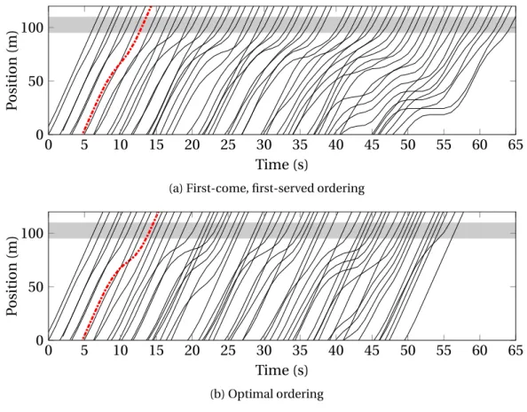
5.5 Comparison of FCFS and optimal ordering . . . 45

5.6 Average delays for optimal and FCFS orderings . . . 46

5.7 Computation time for various gap tolerance levels . . . 46

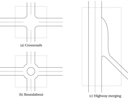
6.1 Road configurations and corresponding supervision area . . . 51

6.2 No stop and acceleration regions . . . 53

6.3 Merging scenario . . . 62

6.4 Intersection crossing scenario. . . 63

6.5 Roundabout scenario. . . 64

6.6 Computation time . . . 65

7.1 Feasible acceleration envelopes. . . 75

7.2 Approximation of feasible accelerations. . . 76

7.3 Modeling of an obstacle as a parabola . . . 78

7.4 Reference path. . . 80

7.5 Comparison of achieved speed . . . 81

7.6 Lateral positioning error . . . 82

7.7 Achieved vehicle speed with obstacles . . . 82

7.8 Lateral deviation . . . 82

7.9 MPC computation time . . . 83

(11)

List of Figures

8.2 Frenet representation of a point on the road . . . 87

8.3 Physical and configuration space representation of obstacles . . . 87

8.4 Configuration space-time for a 3 vehicle scenario . . . 88

8.5 Configuration space-time for a single obstacle . . . 89

8.6 Homotopy classes relative to a region . . . 90

9.2 Guiding example situation. . . 92

9.3 Free space-time in the example situation . . . 93

9.4 Partitioning of the 2D free space . . . 94

9.5 Continuous partitioning of the free space-time . . . 95

9.6 Navigation graph . . . 95

9.7 Discrete partitioning of the free space-time . . . 96

9.8 Discrete-time navigation graph . . . 96

9.9 Trapeze decomposition . . . 98

9.10 Semantic partition around a single obstacle . . . 98

9.11 A more complex example with 3 obstacles. . . 100

10.1 Another partition around a single obstacle . . . 108

10.2 Optimal trajectories with and without time margin . . . 110

11.1 Raw data for the estimation algorithm . . . 122

11.2 Overlay of the LiDAR point cloud on the navigable region . . . 123

11.3 Occupancy predictions . . . 125

11.4 Smoothing of the lateral position and speed. . . 129

11.5 Vehicles of interest around the target vehicle . . . 129

11.6 Internal structure of an LSTM cell . . . 131

11.7 Network architecture used as reference design . . . 132

11.8 Predicted trajectories . . . 133

11.9 Distribution of error on the test set for the bagged predictor. . . 135

11.10 Prediction delay . . . 136

12.1 Representations of occupancy predictions . . . 141

12.2 Decision tree . . . 142

12.3 Simulation results . . . 144

12.4 Reference path. . . 145

12.5 Experimental results . . . 145

A.2 Example of corner-cutting phenomenon . . . A3

A.3 Possible sub-timestep collision between following vehicles . . . A3

B.1 Example of helper constraints . . . B1

B.2 Average relative optimality loss from time step duration . . . B2

B.3 Average relative optimality loss for varying parameters . . . B3

C.1 Overshoot phenomenon . . . C3

D.1 Multiple local optima with a single semi-infinite obstacle . . . D1

D.2 Obstacle modeling as bounding parabola . . . D1

D.3 Simulation model of the vehicle in the (x, y) plane. . . D3

D.4 Feasible accelerations for varying vx . . . D6

D.5 Feasible accelerations for varying vy . . . D7

D.6 Feasible accelerations for varying µ . . . D8

(12)

List of Figures

D.7 Accumulation of samples for low friction coefficient . . . D9

D.8 Variations of the a_Xmi nand a_Xmax . . . D10

E.1 Non-unicity of Xγ . . . E2

(13)

(14)

List of Tables

1.1 US Crash statistics for 2015 . . . 4

1.2 Levels of vehicle automation . . . 5

2.1 Overview of sampling-based algorithms for motion planning . . . 12

7.1 Absolute lateral positioning error for both planners. . . 81

9.1 Validity sets Adj(A,B) . . . 93

9.2 Time margins of example paths . . . 97

10.1 Computation time for 10 time steps . . . 110

10.2 Computation time for 20 time steps . . . 111

11.1 RMS error for the tested models . . . 134

B.1 Parameters used in the studied scenarios . . . B3

(15)

(16)

(17)

(18)

Chapter 1 A primer on automated vehicles

“If I had asked people what they wanted, they would have said faster horses.” Henry Ford

1.1 Context, motivations and challenges

The advent of automobiles has revolutionized personal transportation by giving bil-lions of people to travel almost anywhere on land at a reasonable cost. In 2002, car own-ership levels in western countries were estimated at 0.55 car per capita (OECD average), even raising above 0.8 cars per capita in the United States [1].

Although it certainly is empowering, the actual driving task remains cumbersome, es-pecially in dense traffic or on monotonous highways, prompting car manufacturers to provide increasing amounts of assistance to the driver, with the goal of ultimately provid-ing cars capable of drivprovid-ing without human intervention. However, the disruptive poten-tial of autonomous driving goes well beyond increased comfort.

In Sections1.1.1 and1.1.2, we discuss some of these expected benefits and related challenges, motivating the intense research and engineering effort currently focused on self-driving vehicles and, in particular, motion planning which is at the center of this the-sis. In Section1.1.3, we briefly discuss broader-picture socioeconomic implications of au-tonomous driving. Finally, Section1.1.4, provides a simplified taxonomy of “intelligent” vehicles, in order to help clarify the rest of the thesis.

(19)

Chapter 1. A primer on automated vehicles

1.1.1 Road safety

First, removing the – fallible – human driver by a near-infallible automatic pilot is ex-pected to drastically reduce the occurrence of accidents; in the US alone, roughly 6 mil-lion crashes are reported to the police each year [2], and more than 90% of those can be attributed to human error [3].

Table1.1breaks down the consequence of reported road accidents in the US in 2015, compared to the number of vehicle-kilometers driven on the same year. This table high-lights the remarkably low rate of accidents for human drivers: on average, roughly 10 million kilometers are driven before the occurrence of an accident severe enough to be reported, and almost 200 million before recording a fatality. Due to these extremely low figures, of the major challenges for autonomous driving – although not in the scope of this thesis – lies in the ability to achieve comparable levels of safety, and to demonstrate this performance with a fleet of only dozens of vehicles [4].

Table 1.1 – US Crash statistics for 2015 (computed from data in [2])

Type of accident Number Rate per 108veh. · km

Fatal 32 166 0.646

Injury 1 715 000 34.4

Property damage only 4 548 000 91.3

1.1.2 Traffic efficiency

A second wildly anticipated benefit of autonomous driving is its potential to increase the throughput of existing road infrastructure [5], in hope to reduce congestion. This improvement is thought to be possible due to several complementary aspects.

First, autonomous vehicles are expected to have a much shorter reaction time than human drivers, thus allowing to reduce safety distance or start faster when a traffic light turns green. Moreover, they can also help smooth traffic when nearing saturation, thus delaying the transition towards congestion [6].

Second, vehicle-to-vehicle (V2V) and vehicle-to-infrastructure (V2I) communication can help further improve this efficiency, for instance by allowing vehicles to drive in com-pact platoons [7].

Third, as the penetration rate of autonomous vehicles increases, the infrastructure can be adapted to their improved performance, for instance using narrower lanes or higher speed limits. Finally, in an even longer time frame, some authors have proposed to over-haul traffic management methods such as stop signs or traffic lights, and replace those with so-called Autonomous Intersection Management schemes [8], which allows optimiz-ing the crossoptimiz-ing order of individual vehicles.

1.1.3 Societal and economic impacts

In a broader picture, autonomous driving is expected to have ripple effects across a wide part of society and of the economy [5]. Indeed, self-driving cars promise to grant the same freedom of movement to almost anyone, by allowing elderly or disabled people to use a vehicle by themselves. Going another step further, some authors have proposed that autonomous driving would trigger a shift in vehicle ownership patterns, notably through 4

(20)

1.1. Context, motivations and challenges

Table 1.2 – Levels of vehicle automation (as defined in [10])

Level Name Example

0 No automation Legacy vehicles

1 Driver assistance Adaptive cruise control 2 Partial driving automation Traffic jam assist 3 Conditional driving automation Highway pilot

4 High driving automation City pilot on clear daytime 5 Full driving automation Robot-taxi

an increase of car-sharing [9] which could, in turn, help decrease the amount of driving and parked vehicles in urban centers.

Although autonomous driving is largely praised for its potential benefits, some possi-ble downsides – most of which are discussed in [6] – need also be mentioned. For instance, whether self-driving vehicles will effectively decrease traffic congestion is still debated, as temporarily reduced congestion could also prompt more people to use their own car. Since they can work or rest during their commute, people could also choose to live fur-ther away from their workplace, potentially leading to higher urban sprawl. Due to this induced traffic, the impact on public transportation is more uncertain: although remov-ing the need for a driver may help decrease costs, a reduction in the number of passengers may require higher subsidizing as the poorest population will likely remain excluded from this progress. Similarly, although the ability to operate a vehicle without a driver can be highly appealing to the freight and taxi industry, the loss of employment for professional drivers should also be kept in mind, as well as potential effects in businesses such as in-surance companies.

1.1.4 Taxonomy

Before moving on to the technical aspects of this thesis, we provide a brief overview of the taxonomy of automated or connected vehicles.

Dynamic driving task As defined in SAE International’s J3016 standard [10], the

dy-namic driving task comprises short- and medium-term actions required to operate a

ve-hicle on-road safely. This task includes longitudinal and lateral control, monitoring and interpreting the vehicle’s environment and plan responses to events, as well as planning tactical maneuvers such as lane changes.

Automated vehicles Automated vehicles are vehicles equipped with systems capable of performing parts or all of the dynamic driving task [10]; depending on these capacities, automated driving systems are categorized into six levels as summarized in Table1.2. Note that in order to be considered automated, a vehicle should be able to perform these driving tasks only using its own hardware, and without requiring communication from outside entities.

Legacy vehicles In this thesis, we describe as legacy vehicles with low to no driving au-tomation in a particular situation, mostly corresponding to levels 2 and below. However, this term could also describe vehicles of level 3 or 4 in contexts where their automated driving systems cannot function.

(21)

Chapter 1. A primer on automated vehicles

Autonomous or self-driving vehicles As opposed to legacy vehicles, we use the terms

autonomous or self-driving to designate fully automated vehicles which can function by

themselves without requiring communication. Therefore, this term mostly relates to level 5 vehicles, although it could apply to level 4 systems in contexts where automated driving without human intervention is possible.

Connected vehicles Regardless of their level of automation, vehicles can also be

con-nected – i.e., able to communicate wirelessly either with other vehicles (known as

vehicle-to-vehicle, or V2V communications) or with equipment attached to the road infrastruc-ture (vehicle-to-infrastrucinfrastruc-ture, or V2I). These vehicular communication capacities, com-monly referred to as V2X, can rely on several technologies with various performance [11]. Cooperative vehicles Although vehicular communications can be used in legacy vehi-cles (e.g., to provide traffic information), connectivity is also a means to improve safety and traffic efficiency further than what could be achieved using only automated vehicles. Indeed, communications could allow vehicles to cooperatively – the infrastructure acting as an authority – make and follow decisions such as traveling in platoons [12] or passing intersections autonomously [13]. In this thesis, we use the term cooperative to describe partially or fully automated vehicles capable of using communication to coordinate with others.

1.2 Motion planning in automated vehicles

To close this contextual introduction, we propose to briefly discuss the role of motion planning in automated vehicles. Throughout the rest of this thesis, we use the term

ego-vehicle to designate a particular ego-vehicle, from the viewpoint of which we consider the

driving task.

1.2.1 A classical architecture: the perceive, plan, act paradigm

Automated vehicles are a particular form of wheeled robots; as such, usual approaches to automated driving systems rely on the well-established perceive-plan-act paradigm (see, e.g., [14]). In this framework, a first perception layer is in charge of combining sensor data and potential prior knowledge such as mapping information into a suitable repre-sentation of the state of the ego-vehicle and its environment. The motion planning layer then computes a feasible and efficient trajectory for the ego-vehicle; finally, a control layer activates the vehicle’s actuators to follow this planned trajectory.

1.2.2 An alternative approach: end-to-end learning

With the dramatic increase of available computational power and the undeniable suc-cess of deep learning approaches in applications ranging from computer vision [15] to playing Go [16], a new approach called end-to-end learning has emerged for driving au-tomation. This technique leverages machine learning to design a policy directly comput-ing a sequence of actions (e.g., steercomput-ing angle and acceleration) from raw sensor inputs (e.g., camera images), without requiring human-designed algorithms.

Currently, two major techniques are being investigated for end-to-end driving. In a classical supervised approach (see, e.g., [17]), the algorithm is taught to imitate the be-havior of actual human drivers in given situations, thus requiring a significant amount 6

(22)

1.2. Motion planning in automated vehicles

of training data recorded on real vehicles. More recently, the success of (deep)

reinforce-ment learning algorithms in outreaching human [18] or even AI [19] experts in a variety of tasks without explicitly requiring training data has sparked a vast amount of interest in the artificial intelligence community. In this setting, an agent (the autonomous vehicle) learns through trial-and-error to choose actions maximizing a reward function defined by a human operator. For obvious reasons, reinforcement learning techniques are generally applied in simulations only, and it is unclear how training results can be transferred to the real world.

These methods have the common advantage of considerably simplifying the develop-ment of driving algorithms, and mimic the way humans learn to perform complex tasks. However, they suffer from several downsides that need to be addressed by future research. First, current learning algorithms behave as black boxes with limited interpretability of failure scenarios and no method currently exist to provide behavior guarantees. Second, guaranteeing that trained models will respond well to unseen situations is still an active research topic. Finally, deep learning approaches have been shown to be vulnerable to

(adversarial) attacks, where a tiny modification of the inputs leads to arbitrary changes in

the outputs [20], which can result in security threats. For these reasons, we argue that us-ing intrinsic structural properties of the underlyus-ing problem to guide or constrain learn-ing algorithms is important for safety-critical applications; the results provided in this thesis may therefore constitute a first step towards this goal.

(23)

(24)

Chapter 2 Motion planning

“A good plan implemented today is better than a perfect plan implemented tomorrow.” George Patton (Military)

2.1 Motion planning problems . . . . 9 2.1.1 State representations. . . 10 2.1.2 Path planning . . . 11 2.1.3 Trajectory planning. . . 11 2.2 Motion planning algorithms . . . 12 2.2.1 Sampling-based. . . 12 2.2.2 Optimization-based . . . 12 2.3 Motion planning, homotopy and decision . . . 13 2.3.1 Homotopy classes of paths . . . 13 2.3.2 Divide-and-conquer approaches. . . 14 2.3.3 Motion planning and decision-making . . . 15 2.3.4 Algorithm evaluation. . . 15

2.1 Motion planning problems

The general notion of motion planning refers to the computation of a means for a

system to reach a desired goal starting from a given initial state, and is particularly

impor-tant in the field of robotics [21]. As described in the next subsections, motion planning actually comprises a range of slightly distinct subproblems.

Sources of complexity in general motion planning arise from multiple factors. First, the system generally has to evolve around forbidden regions such as obstacles or off-limits areas, which usually results in non-convex search spaces and multiple local optima can exist [22], as illustrated in Figure2.1a. Second, kinematic constraints on the system such as nonholonomicity1adds another layer of complexity [23] when trying to find feasible

1_{A system is non-holonomic when it has fewer controllable degrees of freedom (DoF) than its total} number of DoF.

(25)

Chapter 2. Motion planning

obstacle

start

goal

(a) Obstacles and non-convexity: multi-ple locally optimal solutions exist

goal

(b) Nonholonomicity: the car cannot directly park in the goal region

Figure 2.1 – Sources of complexity in motion planning

solutions, as illustrated in Figure2.1bin the case of parallel parking. Third, dynamic ef-fects such as slip may have to be taken into account, for instance when dealing with fast or highly precise maneuvers.

2.1.1 State representations

Before presenting different subproblems that fall within the scope of motion

plan-ning, we briefly present a terminology regarding the representations of a system’s “state”.

For the sake of simplicity, we restrict the discussion to systems comprised of a single or multiple mobile robots.

Pose In this thesis, we call pose of a single robot having n degrees of freedom the given of x ∈ Rnfully describing the current position and orientation of the robot’s frame and its joints. For instance, in the case of a simplified 2D vehicle representation, a pose could be given by the vehicle’s position, orientation, and steering angle.

Configuration As introduced in [24], we call configuration of a system of robots the col-lection of the poses of each individual robot in the system. The configuration space C is the set of all configurations. For a single robot, pose and configuration are equivalent. We note Cf the (collision-)free part of the configuration space, i.e. where no collision be-tween robots happens, and Co its complement so that C = Cf ] Co where ] denotes a union of disjoint sets.

The major advantage of using the configuration space is that this formulation allows a reformulation of multi-body collision avoidance constraints as simpler point-outside-polygon problem (assuming point-outside-polygonal obstacles) or point-outside-region in the general case, as illustrated in Figure 2.2. A standard approach in motion planning is to use the Minkowski difference to compute the collision-free space [25].

State We call state X of a system (either a single or multiple robots) the given of its con-figuration x and its time derivatives up to a sufficient order, such that the dynamics of the system (without any form of control) can be expressed as a differential equation ˙X = f0(X).

The state space X is the set of all states; we denote by Xf the free portion of the state space, i.e. the set ©X ∈ Xf¯

¯Π_C(X) ∈ Cf ª

where ΠC(X) denotes the projection of X in the

configuration space. 10

(26)

2.1. Motion planning problems

(a) Geometric space (b) Configuration space

Figure 2.2 – Comparison of planning in the geometric space and in the configuration space

goal

start

(a) Path planning

goal

start

(b) Trajectory planning

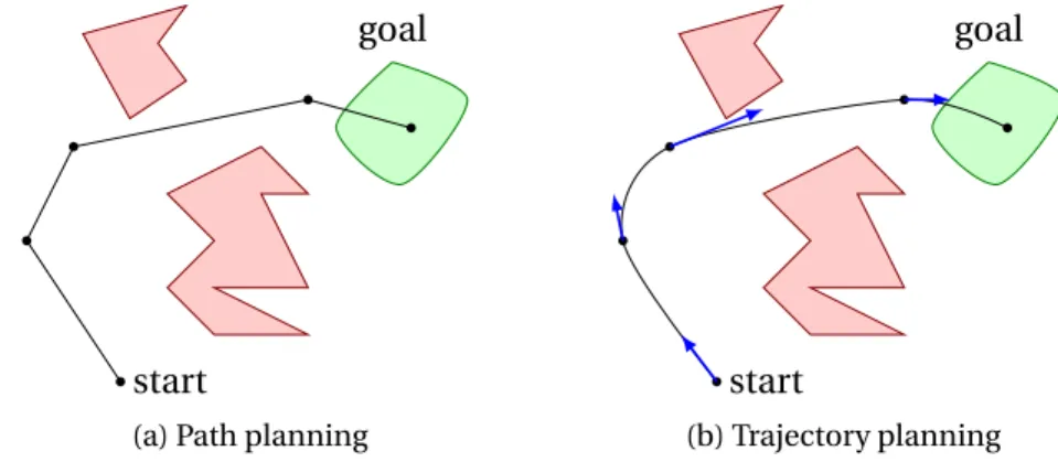
Figure 2.3 – Examples of motion planning problems; red polygons represent obstacles.

Control We call control u an input to the system that can change the evolution of its state, such that under this control ˙X = f (X,u). We note U the set of all admissible controls,

i.e. which are actually feasible by the system.

2.1.2 Path planning

The path planning problem corresponds to finding a (collision-free) path between an initial configuration x0∈ Cf and a target region Xg oal 6= ; (possibly a single point) with

Xg oal _{⊂ C}f _{is that of finding a continuous function f : [0,1] → C}f _{such that f (0) = x}

0

and f (1) ∈ Xg oal. Figure2.3apresents a possible path for a point-mass system among obstacles inR2_.

Note that, although it is the simplest form of motion planning problems, path plan-ning amidst obstacles is known to be NP-hard [26], with a complexity growing exponen-tially in the number of obstacles.

2.1.3 Trajectory planning

The trajectory planning problem is the time-based equivalent of path planning, ap-plied in the state space. For an initial state X0∈ Xf and a non-empty goal region Xg oal⊂

Xf, the trajectory planning problem2is that of finding a function g : [0,+∞] → Xf with

f (0) = X0and ∃T > 0 such that ∀t ≥ T, f (t) ∈ Xg oal. A trajectory is said to be (dynamically)

feasible if there exists an admissible control u : [0,T] → U realizing this trajectory.

2_{In the case of static obstacles}

(27)

Note that the trajectory planning problem can conveniently be cast as a path planning one in the “state-time space”R+×Xf, with the first dimension representing time, and

us-ing the added constraint that the first component of the path should be strictly increasus-ing. This approach also allows handling the case of moving obstacles by considering the free portion of the state-time space ©(t,X) ∈ R+× X¯¯X ∈ Xf(t)ª, where Xf(t) denotes the free portion of the state space at time t [27,28].

2.2 Motion planning algorithms

Due to the existence of obstacles which effectively cause the search space to be non-convex, generic motion planning in an arbitrary space is an NP-hard problem. basically corresponding to the choice of a maneuver variant [29]. In this section, we present an overview of the existing literature on motion planning algorithms; these techniques can be grouped as either sampling-based or optimization-based [30,31].

2.2.1 Sampling-based

Sampling-based algorithms are often used to deal with NP-hard problems, as they guarantee a fixed runtime and can have interesting properties such as asymptotic com-pleteness (ensuring that a solution can eventually be found) or asymptotic optimality (en-suring that the best solution found converges to the optimum as the number of samples increases). In the motion planning literature, sampling-based algorithms can be further distinguished based on whether samples are chosen deterministically or randomly, and whether samples correspond to system states or controls. Table2.1presents an overview of different sampling-based algorithms used in motion planning. A more detailed review of existing algorithms can be found, e.g., in [30].

Apart from these differences, sampling-based algorithms all operate on the same prin-ciple: a predetermined number of samples is chosen in the sampled space, and the corre-sponding trajectories are then evaluated with respect to a chosen cost function – possibly using forward integration in the case of samples in the control space. The best trajectory for this cost function is then selected.

One of the main downsides of sampling-based approaches is that they ignore the ex-istence of maneuver variants, which are never considered explicitly. Therefore, these al-gorithms have a high risk of being trapped around local optima without even exploring certain configurations.

2.2.2 Optimization-based

In this review, we use the term optimization-based to describe techniques based on directly using mathematical programming (e.g., constrained optimization) for the motion planning problem.

Table 2.1 – Overview and classification of sampling-based algorithms for motion planning

Random sampling Deterministic sampling

State space PRM [32], RRT [33] State lattices [34], motion primitives [35] Control space MPPI [36] Mobile automaton [37]

(28)

2.3. Motion planning, homotopy and decision

In particular, Model Predictive Control (MPC) techniques – although originally de-signed for control systems – has been extensively used in motion planning (see, e.g., [38]). In this framework, motion planning is formulated as an optimization problem where the system’s dynamics are used as constraints alongside with obstacle avoidance require-ments. For real-time tractability, this optimization problem is usually solved over a finite time horizon, and replanning is frequently used to take uncertainty and new informa-tion into account. Although it has been demonstrated to work well in practice, a partic-ular problem of model predictive control lies in guaranteeing infinite horizon properties (e.g., recursive feasibility) whereas the formulation only considers a finite planning hori-zon [39]. A possible approach to provide such guarantees lies in the use of invariant sets theory (see, e.g., [40]); however, finding such invariant sets may be difficult for complex systems or dynamic environments, and this verification is rarely performed in practice.

Another difficulty when using MPC methods for motion planning is linked to the in-trinsic NP-hardness of the problem, and the modeling of obstacle-related constraints is paramount to the actual computability of the problem. A possible approach is to model obstacles as holes (usually rectangles or ellipses) in the search space, and use gradient descent to perform the actual optimization (see, e.g., [14]). However, as with sampling-based approach, the non-convexity of the search space implies a high probability of these approaches resulting in a local optimum [29].

Note that, although this section mostly focused on MPC, other optimization-based approaches, such as potential-field methods [41], have also been used for path planning, although their generalization to time-dependent problems may be difficult.

2.3 Motion planning, homotopy and decision

As mentioned earlier, one of the major challenges of motion planning lies in the non-convexity of the search space in the presence of obstacles. A particularly powerful tool to help describe this complexity is linked to the notion of homotopy classes, which has re-cently been leveraged in divide-and-conquer approaches to motion planning for a single-or multi-robots systems [42,43,29].

2.3.1 Homotopy classes of paths

In the case of a single robot navigating among obstacles, it has long been known that the uncountable set of collision-free paths between a given start and end point can be partitioned into a countable3number of homotopy classes [44]. Mathematically, two paths having the same start and end points are said to be homotopic if they can be continuously deformed into one another while remaining in Cf, as illustrated in Figure2.4.

The notion of homotopy allows defining an equivalence relation between collision-free paths [45]: two such paths – sharing the same start and end points – are said to be equivalent if they are homotopic. This equivalence relation in turn defines a partition of the set of collision-free paths into homotopy classes. In the example of Figure2.4, and if requiring the paths to have an increasing horizontal component, only two classes of paths can be distinguished as avoiding the obstacle “from above” of “from below” (Figure2.4a). If monotonicity is not required, there exist a (countable) infinity of classes corresponding to an arbitrary number of loops around the obstacle (Figure2.4b).

3_{Or finite if at least one coordinate is required to vary monotonously}

(29)

obstacle

start

goal

(a) Monotonous case (no loop)

obstacle

start

goal

(b) Non-monotonous case (loops)

Figure 2.4 – Homotopy classes for paths around an obstacle. The blue paths are homotopic since they can be continuously deformed into one another (dashed paths), but cannot be deformed into the green path without entering the obstacle region.

Figure 2.5 – Decomposition of the path planning problem in sequences of convex cells (from [43]).

However, the use of homotopy classes is shown in Chapter8 to be poorly suited to encode decisions in the case of autonomous driving, where lateral vehicle movement is not monotonous. For this reason, other approaches are required to properly describe the discrete component of motion planning.

2.3.2 Divide-and-conquer approaches

Divide-and-conquer strategies have been applied very early in order to decompose motion planning into simpler subproblems, and show promising potential to generalize the notion of homotopy.

The so-called path-velocity decomposition [46] – consisting in first choosing a collision-free path, then planning the velocity of the system along this path – is a form of divide-and-conquer approach, which has been highly successful in motion planning. However, this approach is difficult to generalize in the case of moving obstacles.

More recently, some authors have proposed a geometric decomposition of the path planning problem with fixed obstacles with interesting results [43], as illustrated in Fig-ure2.5. In doing so, they create a graph-based representation of the free space; paths in this graph are shown to bijectively correspond to homotopy classes of collision-free paths. Decomposition-based approaches have also been used in the field of multi-robot co-14

(30)

2.3. Motion planning, homotopy and decision

Figure 2.6 – Homotopy classes in a 3-robot coordination problem. Axes correspond to the curvi-linear xi position of robot i along a predetermined path; cylinders represent the obstacle region

where two robots would collide (from [42]).

ordination using the notion of “priorities”, which exactly correspond to specifying a ho-motopy class in an N-robots coordination space, as illustrated in Figure2.6[42].

2.3.3 Motion planning and decision-making

In this thesis, we argue that the reason for the success of these divide-and-conquer ap-proaches in the field of motion planning lies in the fact that homotopy classes are intrin-sically linked to discrete decisions relative to how obstacles should be avoided in certain particular cases. Making such a decision essentially corresponds to solving the discrete portion of the planning problem; once done, usual continuous optimization techniques can be effectively used to find an optimal trajectory within the corresponding class.

Therefore, there are undeniable advantages to using an explicit or implicit represen-tation of the possible decisions to solve motion planning problems in complex scenarios such as the navigation of a self-driving vehicle in an urban setting, or the coordination of cooperative vehicles in critical parts of the road infrastructure such as intersections or roundabouts.

However, we show in Chapter8that the notion of homotopy does not always overlap with driving decisions, especially in the case of motion planning for autonomous vehicles. To the best of our knowledge, no framework exists to enumerate and represent driving de-cisions, let alone use them efficiently for motion planning. One of the major contributions of this thesis is the introduction of a mathematical framework allowing systematic enu-meration of driving decisions in generic situations, as well as algorithms building upon this framework for autonomous motion planning.

2.3.4 Algorithm evaluation

As a final consideration before closing this introductory chapter, let us point out that motion planning has an extremely wide range of applications, and the idea of a “one-size-fits-all” motion planning algorithm seems illusory with respect to the current state of the art.

(31)

In the case of automated driving, we argue that real-time performance is more impor-tant than the optimality of the output. As a result, the ability of an algorithm to rapidly find a solution of acceptable quality is paramount. A second performance criterion is the ability of the algorithm to progressively improve the quality of the solution, ultimately converging towards the actual optimum given enough time; third, the speed of this con-vergence is also important.

Another aspect to be taken into account is that the “optimality” of the solution obvi-ously depends on the objective function used to evaluate it. Although determining what makes a trajectory desirable or not is out of the scope of this thesis, we wish to point out that different kinds of algorithms or problem representations may allow different levels of expressivity in the objective function. In particular, we show in Chapter9that carefully crafted problem formulations can provide access to metrics such as margin for error – which is arguably an important evaluation criterion, but is not easily taken into account in other planning frameworks.

(32)

Chapter 3 Contributions and thesis outline

“ Basic research is like shooting an arrow in the air and, where it lands, painting a target. ” Homer B. Adkins (Chemist)

As introduced in the previous chapter, one of the main challenges of motion planning originates from the discrete choices regarding how each obstacle should be avoided, ef-fectively resulting in a combinatorial problem. In this thesis, we advocate that a good mathematical representation of these choices is key to improve the performance and ro-bustness of planning algorithms, thus stressing the importance of decision-making in this context; the thesis provides three main contributions to existing knowledge, both in the field of cooperative and autonomous driving.

3.1 Cooperative driving

In the case of cooperative driving of fully autonomous vehicles, a previous thesis stud-ied Priority-based coordination of mobile robots [42] and evidenced that the given of pair-wise precedence relations between robots were necessary and sufficient to fully define a single homotopy class of collision-free (system) trajectory. In reference [42], priority re-lations are described as a plan to be executed in order to properly coordinate the robots, and a simple priority-preserving control was proposed to effectively allow the robots to comply with this ordering. However, efficient priority assignment policies have not been yet been proposed.

A first contribution of the present thesis is the proposal of an optimal decision-making algorithm to coordinate autonomous or semi-autonomous robots, that builds upon and extends the priority framework of [42]. In Chapter4, we establish the link between this priority framework and decision-making in the case of multi-robots coordination, and propose a mixed-integer programming approach to decision-making. This technique is

(33)

Chapter 3. Contributions and thesis outline

then adapted to the case of optimal coordination of autonomous robots in Chapter5, or to the supervision of semi-autonomous vehicles in Chapter6.

By allowing the use of powerful optimization methods such as mixed-integer pro-gramming, this decision-making framework is shown to be capable to output real-time optimal coordinated trajectories for up to a dozen of robots. Besides cooperative driving, we forecast potential applications to a much wider range of scenarios, including auto-mated warehouses or guided transportation.

3.2 Autonomous driving

The second major contribution of this thesis is a generic framework to describe the discrete choices involved in motion planning in the case of autonomous driving, i.e. with numerous mobile obstacles in a relatively structured environment. This framework, gen-eralizing that of [43], allows encoding the whole decision-making problem as a “shortest-path search” in a navigation graph, as presented in Chapter9; Chapter10presents exact and heuristic approaches to use this mathematical framework for actual motion plan-ning.

To the best of our knowledge, this framework is the first to allow systematic enumer-ation and evaluenumer-ation of possible driving decisions in generic situenumer-ations. Previous studies usually assimilate these decisions with homotopy classes of trajectories [43,29]; however, this notion is shown in Chapter8to be insufficient in the context of autonomous motion planning. By contrast, this thesis proposes to generalize this mathematical notion into a decision-making framework explicitly designed for the needs of autonomous driving, opening exciting perspectives to incorporate recent machine learning approaches while guaranteeing vehicle safety.

3.3 Towards practical implementation

Finally, the third part of this thesis focuses on feeding the decision-making algorithms in order to bridge the gap between theory and practice. Indeed, a large part of the motion planning literature has focused on simulation results with perfect or near-perfect sens-ing capacities, which is far beyond the current state-of-the-art of perception systems for automated vehicles. In Chapter 11, we present early approaches to estimate probable, short-term future trajectories for surrounding vehicles, which we argue is a cornerstone requirement for fully automated driving. Finally, Chapter12 presents a simplified real-world implementation of our decision-making algorithms to a peri-urban driving sce-nario serving as a proof-of-concept for the ideas developed throughout the thesis.

3.4 Publications

Most of the results presented in this thesis have been published as conference or jour-nal articles; the list below presents these publications and indicates, when applicable, the corresponding chapter in the thesis.

Articles used as basis for thesis chapters

• F. Altche, X. Qian, and A. de La Fortelle, “Time-optimal coordination of mobile robots along specified paths,” in 2016 IEEE/RSJ International Conference on Intelligent Robots 18

(34)

3.4. Publications

and Systems (IROS), pp. 5020–5026, IEEE, oct 2016 (used in Chapter5)

• F. Altché and A. de La Fortelle, “Analysis of optimal solutions to robot coordination problems to improve autonomous intersection management policies,” in 2016 IEEE

Intelligent Vehicles Symposium (IV), vol. 2016-August, pp. 86–91, IEEE, jun 2016 (used

in Chapter5)

• F. Altché, X. Qian, and A. de La Fortelle, “Least restrictive and minimally deviat-ing supervisor for Safe semi-autonomous drivdeviat-ing at an intersection: An MIQP ap-proach,” in 2016 IEEE 19th International Conference on Intelligent Transportation

Systems (ITSC), pp. 2520–2526, IEEE, nov 2016 (used in Chapter6)

• F. Altche, X. Qian, and A. de La Fortelle, “An Algorithm for Supervised Driving of Cooperative Semi-Autonomous Vehicles,” IEEE Transactions on Intelligent

Trans-portation Systems, vol. 18, pp. 3527–3539, dec 2017 (used in Chapters4and6) • F. Altché, P. Polack, and A. de La Fortelle, “A Simple Dynamic Model for Aggressive,

Near-Limits Trajectory Planning,” in 2017 IEEE Intelligent Vehicles Symposium (IV), pp. 1–6, 2017 (used in Chapter7)

• F. Altche, P. Polack, and A. de La Fortelle, “High-speed trajectory planning for au-tonomous vehicles using a simple dynamic model,” in 2017 IEEE 20th International

Conference on Intelligent Transportation Systems (ITSC), pp. 1–7, IEEE, oct 2017 (used

in Chapter7)

• F. Altche and A. de La Fortelle, “Partitioning of the free space-time for on-road nav-igation of autonomous ground vehicles,” in 2017 IEEE 56th Annual Conference on

Decision and Control (CDC), pp. 2126–2133, IEEE, dec 2017 (used in Chapters 9

and10)

• F. Altche and A. de La Fortelle, “An LSTM network for highway trajectory predic-tion,” in 2017 IEEE 20th International Conference on Intelligent Transportation

Sys-tems (ITSC), pp. 353–359, IEEE, oct 2017 (used in Chapter11)

Collaborations not presented in this thesis

• X. Qian, F. Altché, P. Bender, C. Stiller, and A. de La Fortelle, “Optimal trajectory plan-ning for autonomous driving integrating logical constraints: An MIQP perspective,” in 2016 IEEE 19th International Conference on Intelligent Transportation Systems

(ITSC), pp. 205–210, IEEE, nov 2016

• X. Qian, F. Altché, J. Gregoire, and A. de La Fortelle, “Autonomous Intersection Man-agement Systems: Criteria, Implementation and Evaluation,” IET Intelligent

Trans-port Systems, feb 2017

• P. Polack, F. Altche, B. D’Andrea-Novel, and A. de La Fortelle, “The kinematic bicycle model: A consistent model for planning feasible trajectories for autonomous vehi-cles?,” in 2017 IEEE Intelligent Vehicles Symposium (IV), pp. 812–818, IEEE, jun 2017 • P. Polack, F. Altché, B. D’Andréa-Novel, and A. de La Fortelle, “Guaranteeing Con-sistency in a Motion Planning and Control Architecture Using a Kinematic Bicycle Model,” in Proceedings of the American Control Conference, jun 2018

(35)

(36)

Part I

(37)

(38)

Introduction

The first part of this thesis expands on the results on priority-based coordination of multiple mobile robots [42] to illustrate the role of decision-making in cooperative mo-tion planning for multiple vehicles. In a multi-robot coordinamo-tion problem, a set of co-operative mobile robots having individual goals (e.g., a destination) have to share a finite resource (namely, ground space) as efficiently as possible. This problem is of particu-lar interest for autonomous intersection management, where vehicles cooperate with one another or with the road infrastructure in order to improve safety and efficiency at road intersections over more classical techniques such as traffic lights. Although we use the generic term of robot for the sake of generality, the discussion can of course be applied to fully (and, in some instances, partially) automated vehicles as well.

Multi-robot coordination can be considered from two complementary viewpoints, which lead to widely different solving algorithms. A first approach is to consider coordi-nation as a resource allocation problem to be solved using job scheduling algorithms [59] or queuing theory (see, e.g., [60]). A second method (see, e.g., [61]) is to model the multi-robots coordination problem as that of planning a collision-free trajectory for a system of mobile robots, and hence falls into the class of motion planning problems. In the follow-ing chapters, we adopt this second point of view in the followfollow-ing chapters; the compared advantages and downsides of both formulations are compared in Chapter5.

As presented in Chapter2, priorities are a convenient way to encode homotopy classes of collision-free trajectories for the system of vehicles, which effectively correspond to discrete choices between relative vehicle orderings. The first contribution of this thesis is the use of priority relations within the framework of mathematical (or, more precisely, mixed-integer) programming to achieve optimal coordination of the vehicles. The result-ing framework is highly versatile, and the use of well-chosen objective functions allows achieving widely different goals.

In this thesis, we argue that the performance and versatility of this framework are made possible by the choice of a proper representation of the intrinsic decisions involved in the motion planning problem. In this case, decisions are encoded as priority relations or, equivalently, as homotopy classes.

Sketch of PartI This part is divided into three chapters. Chapter4 lays the founda-tions of our priority-based framework for cooperative decision-making of multiple robots, which we then use throughout the rest of PartI. A first application of this approach to optimal coordination of automated vehicles is then presented in Chapter5; in this case, vehicles act as a slave to an authority which prescribes their driving speed through an in-tersection in order to optimize its throughput. In Chapter6, we choose a slightly different cost function which results in a widely different behavior known as supervised driving: in this case, the authority only acts to correct driver errors which would otherwise inevitably lead to a collision.

(39)

(40)

Chapter 4 Priority-based cooperative

decision-making

“ In any moment of decision, the best thing you can do is the right thing. The worst thing you can do is nothing. ” Theodore Roosevelt

4.1 Multi-robot coordination and motion planning . . . 25 4.2 Priority and decision-making. . . 26 4.3 Mixed-integer programming . . . 28 4.4 Modeling priorities . . . 28 4.4.1 Conflict regions . . . 29 4.4.2 Subregion indicators . . . 30 4.4.3 Priority variables . . . 32 4.5 Dynamic constraints . . . 34 4.6 Chapter conclusion. . . 35

4.1 Multi-robot coordination and motion planning

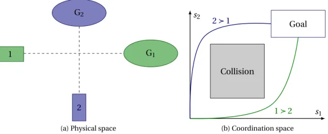
The problem of multi-robot coordination is that of best sharing a finite resource – in this case, space – to allow multiple mobile robots to reach their respective goals without colliding with one another. Figure4.1illustrates a simple example of a two-robots coordi-nation problem: robots 1 and 2 respectively try to reach their goal region G1and G2, but

have a potential conflict where the black dashed paths intersect.

In the example of Figure4.1, a possible solution to avoid conflict would be to have robot 2 follow the dotted red path going around robot 1, effectively removing the risk of collision. However, automated driving applications are usually constrained to existing roads and lanes, which highly restricts the applicability of so-called deconfliction tech-niques, which are mostly used for unmanned aerial vehicles (UAVs) [62,63]. For this rea-son, the rest of the discussion focuses on coordinating robots along fixed paths, for in-stance the centerline of a road lane; this hypothesis simplifies the coordination problem into a simpler velocity planning one.

(41)

Chapter 4. Priority-based cooperative decision-making

1

2 G2

G1

Figure 4.1 – Example of a two-robot coordination problem

Throughout the rest of PartI, we consider that each robot i has a given reference path γi :R → C_if which is a (continuous) function of the curvilinear abscissa s such that γi(s) is the reference configuration of i after traveling a distance s along the path starting from an arbitrary reference point. In this case, C_if is the free portion of the configuration space of robot i when considered alone, i.e. we only require that following the reference path does not lead to a collision with a static obstacle; however, reference paths of two distinct robots can be conflicting, as it is the case for the black dashed paths shown in Figure4.1.

A useful representation to describe collisions between robots is to consider the config-uration space for the system of robots, sometimes called coordination space (see, e.g., [64, 65]), which we denote by χ. The free portion of the coordination space, χf, is a subset of Q_{i ∈R}C_if, but does not contain the sets of configurations leading to collisions between robots. Using this space, we can now define the fixed-path coordination problem as fol-lows:

Problem 1 (Multi-robot coordination along fixed paths). We consider a (finite) set of

mo-bile robots R at time t0, with robot i traveling along a fixed path γi:R → C_if. We denote by

x0

i ∈ γi(R) the configuration of robot i at t0, and assume that each robot has a non-empty

goal region Gi ⊂ γi(R).

The multi-robot coordination problem is that of finding a continuous velocity profile

s = (si)_{i ∈R}for the system of robots such that:

i. for all i ∈ R, γi(si(t0)) = x0_i,

ii. for all t ≥ t0, ¡γi(si(t))¢_{i ∈R}⊂ χf,

iii. there exists T ≥ t0such that, for all t ≥ T and all i ∈ R, γi(si(t)) ∈ Gi.

We call T the completion time of the problem.

4.2 Priority and decision-making

Since the reference paths γi are given and assumed to be perfectly followed by the robots, Problem1can be formulated using curvilinear abscissas, leading to a “path-finding” problem in an abstract space where each dimension corresponds to the curvilinear posi-tion of one robot. For the sake of simplicity, we do not make explicit distincposi-tions between 26

(42)

4.2. Priority and decision-making

1

2 G2

G1

(a) Physical space

Collision s1 s2 Goal 1 Â 2 2 Â 1 (b) Coordination space

Figure 4.2 – Correspondence between the physical and the coordination space in a two-robots example

these two representations and we consider curvilinear abscissas and the corresponding robot configurations as equivalent1_.

In this section, we present the so-called priority framework introduced in [42], upon which our decision-making algorithm is built, through an example. Figure4.2presents the modeling of a real world two-robots coordination problem as a pathfinding problem in the abstract coordination space. The red “Collision” area in Figure4.2bcorresponds to the conflict region at the intersection of the robots’ paths and is excluded from the free space χf_{. Paths in the coordination space such as shown in green and blue in can then be} mapped to collision-free trajectories for the robots2.

As was discussed in Chapter 2, the blue and green paths shown in Figure 4.2b cor-respond to two distinct homotopy classes of paths, namely those avoiding the collision region “from below” (blue path, corresponding to robot 1 crossing before robot 2, and denoted by 1 Â 2) or “from above” (green path, corresponding to robot 2 crossing before robot 1 and denoted by 2 Â 1). The name “priority” stems from the relationship between these homotopy classes, and relative ordering of the robots. As demonstrated in [42], this observation generalizes to an arbitrary number of robots: any homotopy class of collision-free paths can be uniquely described by the given of pairwise priority rela-tions between conflicting robots.

In this thesis, we argue that explicitly using this knowledge about homotopy classes allows designing more efficient motion planners, as they provide a proper description of the decision-making process which has to be undertaken when actually planning a trajectory. The following sections present our proposed approach to treat the challenging question of priority assignment, which remained unanswered in reference [42].

1_{This slight abuse of language may only be problematic for reference paths containing loops, for which} the mapping from curvilinear abscissa to configuration is not injective. In this case, additional information is required to map a configuration to a single curvilinear abscissa.

2_{More specifically, for a path g : [0,1] → χ}f_{, a collision-free trajectory can be obtained from g (u(t)) for}

any continuous function u :R → [0,1]. The dynamic feasibility of this trajectory, however, depends on a proper choice of u; this aspect is discussed in Section4.5.

(43)

Chapter 4. Priority-based cooperative decision-making

4.3 Mixed-integer programming

Motion planning usually concerns with finding efficient trajectories, and therefore is intimately linked with (constrained) optimization. As was presented in Chapter2, non-convexity of the search space is one of the main challenges in this regard, and the use of priorities is an effective way of decomposing the difficult, non-convex motion planning problem into smaller (but numerous) convex subproblems. Indeed, as decisions corre-spond to assignments of pairwise priority relations between robots, the number of pos-sible assignments for N robots can be as large as 2N(N−1)/2_{; this upper bound is reached,}

for instance, for N robots on pairwise-distinct paths all intersecting at the same point. However, in more classical situations, many of these possibilities can be discarded as physically unfeasible (e.g., a robot having to go through another) or as inefficient (e.g., introducing unnecessarily long delays by waiting for a robot far away from the conflict point).

A possible way of handling this combinatorial explosion is, therefore, to prune the corresponding decision tree by removing provably suboptimal or infeasible branches. Mixed-integer programming (MIP) is a widely-used framework that allows efficient han-dling of such combinatorial problems. General MIP problems involving arbitrary func-tions are very hard, but good techniques exist for a subclass of these problems, called mixed-integer second-order cone programming, or MISOCP [66]. In these problems, a convex quadratic objective function is minimized with quadratic positive semi-definite or affine constraints. A better-known subclass of MISOCP is mixed-integer linear (MILP) or quadratic (MIQP) programming. In this subset of problems, all constraints are required to be linear (possibly involving integer variables), and the objective function is also required to be linear in the MILP variant. These techniques have already been applied to trajectory planning in general, and to the multi-robots coordination problem in particular; a review of existing literature and a comparison with our approach is presented in Chapter5. A description of MILP/MIQP3solving algorithms can be found, for instance, in [67].

Several equivalent formulations of MIQP are commonly found in the literature; in this thesis, we define an MIQP problem as follows:

Problem 2 (MIQP). We call mixed-integer quadratic programming an optimization

prob-lem of the form

Minimize x∈Rn x T_{Qx + q}T_x subject to Aex = be, Agx + bg≥ 0, ∀i ∈ I, xi∈ Z ,

where matrix Q is positive semi-definite and I ⊂ {1,...,n} is used to enforce integrality con-straints on certain components of x. If Q = 0, the above problem is an instance of mixed-integer linear programming.

4.4 Modeling priorities

Due to the success of MIQP methods in multiple fields of operations research, we pro-pose to model the priority relations within the mixed-integer linear-constraints

frame-3_{For brevity purposes and since MILP is a subclass of MIQP, we choose the latter to represent both types} of problems, although MILP formulations are quite easier to solve and therefore are frequently preferred.

(44)

4.4. Modeling priorities

work in order to leverage these techniques for actual resolution. As introduced in Sec-tion4.2, we only need consider relative orderings within pairs of robots; in what follows, we use the curvilinear abscissa si(jointly with the reference path γi) to encode the config-uration of each robot i ∈ R, as in Figure4.2. Moreover, we discretize the problem in time with a fixed time step duration τ, and we denote by sk_i the position of robot i at time step

k (corresponding to time kτ).

4.4.1 Conflict regions

We first define two regions of interest in the coordination space4:

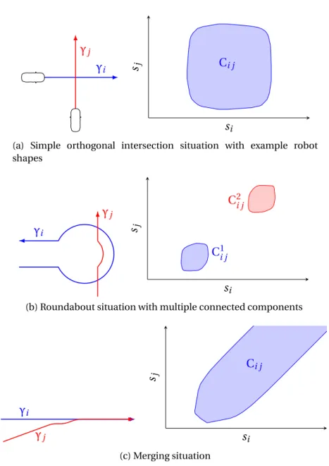
Definition 1 (Collision region). For two robots i and j ∈ R, we note Ci j ⊂ R2 the set of

positions (si, sj) where the two robots would collide, called collision region.

In general, Ci j can be empty (e.g., for robots on parallel paths) or have one or several connected components (e.g., for paths with multiple intersection points). When Ci j has multiple connected components, we denote by C_{i j}p its p-th component, using the con-vention C_{i j}p = Cp_{j i}. Figure4.3illustrates the shape of the obstacle region5 in the case of car-like robots traveling in different road configurations.

Definition 2 (Conflict region). For two robots i and j ∈ R, we call conflict region between

R ×{sj}¢ ∩ Ci j6= ;ª

.

By this definition, two robots are in their conflict region when there is a possibility of collision between them; of course, the collision region is contained within the conflict region.

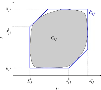
Since the paths and shapes of each robot is known in advance, it is possible to com-pute the collision regions offline using, e.g., Minkowski difference. Interestingly, each con-nected component of the collision regions can be approximated efficiently in the shape of a hexagon with edges either horizontal, vertical or parallel to the identity line, denoted by ˆCi j in Figure4.4. Schematically, the horizontal (respectively, the vertical) edge corre-sponds to having robot j (respectively i ) wait for robot i (resp. j ) to fully pass the conflict point before moving forward. The diagonal edges correspond to requiring the rear robot to maintain a minimum distance from the lead one, for instance in merging or following situations. AppendixA.1describes a linear-time algorithm to compute minimum bound-ing hexagons from a list of points definbound-ing the collision regions.

To simplify notations6_{, we consider a collision region having a single connected}

com-ponent and drop the superscript p; note that the results still hold in the case of multiple connected components by applying the described method for each component p. We also assimilate the exact collision region Ci j with its hexagonal approximation ˆCi j. We denote by s⊥

i j, si j∥ and s⊥i j (and their j i counterparts) the coordinates of different vertices of the bounding hexagon, as shown in Figure4.4.

4_{As they only refer to pairs of robots, Definitions}₁_and₂_{correspond to the projection A of a set ˜A} of the form A × Rn−2⊂ C ⊂ Rn (with a possible reordering of the coordinates), ontoR2_{. To simplify the} presentation, we assimilate ˜A with A.

5_{Strictly speaking, Figure}_4.3_{shows the convex envelope of these regions, which we will use as an} ap-proximation of their exact shape.

6_{This simplification was implicit in Figure}_4.4_.

Decision-based motion planning for cooperative and autonomous vehicles

HAL Id: tel-02073593

https://pastel.archives-ouvertes.fr/tel-02073593

Decision-based motion planning for cooperative and

autonomous vehicles

Florent Altche

To cite this version:

THÈSE DE DOCTORAT

de l’Université de recherche Paris Sciences et Lettres

PSL Research University

Préparée à MINES ParisTech

Decision-based motion planning for cooperative and autonomous

vehicles

École doctorale n

o

432

Spécialité

Soutenue par

Florent A

LTCHÉ

le 30 août 2018

Dirigée par

Arnaud

LA

FORTELLE

Abstract

Contents

Introduction

3

I Cooperative motion planning

21

II Motion planning for autonomous driving

69

III Beyond simulations: bridging the gaps

115

IV Appendices

169

List of Figures

List of Tables

Chapter 1

A primer on automated vehicles

Contents

1.1 Context, motivations and challenges

1.1.1 Road safety

1.1.2 Traffic efficiency

1.1.3 Societal and economic impacts

1.1.4 Taxonomy

1.2 Motion planning in automated vehicles

1.2.1 A classical architecture: the perceive, plan, act paradigm

1.2.2 An alternative approach: end-to-end learning

Chapter 2

Motion planning

Contents

2.1 Motion planning problems

2.1.1 State representations

2.1.2 Path planning

2.1.3 Trajectory planning

2.2 Motion planning algorithms

2.2.1 Sampling-based

2.2.2 Optimization-based

2.3 Motion planning, homotopy and decision

2.3.1 Homotopy classes of paths

2.3.2 Divide-and-conquer approaches

2.3.3 Motion planning and decision-making

2.3.4 Algorithm evaluation

Chapter 3

Contributions and thesis outline

Contents

3.1 Cooperative driving

3.2 Autonomous driving

3.3 Towards practical implementation

3.4 Publications

Articles used as basis for thesis chapters

Collaborations not presented in this thesis

Part I

Introduction

Chapter 4

Priority-based cooperative

decision-making

Contents