HAL Id: tel-02096788
https://pastel.archives-ouvertes.fr/tel-02096788
Submitted on 11 Apr 2019HAL is a multi-disciplinary open access archive for the deposit and dissemination of sci-entific research documents, whether they are pub-lished or not. The documents may come from teaching and research institutions in France or abroad, or from public or private research centers.
L’archive ouverte pluridisciplinaire HAL, est destinée au dépôt et à la diffusion de documents scientifiques de niveau recherche, publiés ou non, émanant des établissements d’enseignement et de recherche français ou étrangers, des laboratoires publics ou privés.
control systems for autonomous driving
Philip Polack
To cite this version:
Philip Polack. Consistency and stability of hierarchical planning and control systems for autonomous driving. Automatic. Université Paris sciences et lettres, 2018. English. �NNT : 2018PSLEM025�. �tel-02096788�
de l’Université de recherche Paris Sciences et Lettres
PSL Research University
Préparée à MINES ParisTech
Consistency and stability of hierarchical planning and control systems for
autonomous driving
Cohérence et stabilité des systèmes hiérarchiques de planification et de
contrôle pour la conduite automatisée
École doctorale n
o
432
SCIENCE DES MÉTIERS DE L’INGÉNIEUR
Spécialité
MATHÉMATIQUES ET INFORMATIQUE TEMPS-RÉELSoutenue par
Philip P
OLACK
le 29 octobre 2018
Dirigée par
Brigitte
D’A
NDRÉA-N
OVEL ETA
RNAUD DEL
AF
ORTELLECOMPOSITION DU JURY :
M Alain Oustaloup
Univ. Bordeaux, Président du jury M Thierry-Marie Guerra
Univ. Valenciennes, Rapporteur M Philippe Martinet
Inria Sophia Antipolis, Rapporteur M Ming Yang
Univ. Shanghai Jiao-Tong, Membre du jury Mme Brigitte d’Andréa-Novel
Mines ParisTech, Membre du jury M Arnaud de La Fortelle
Autonomous vehicles are believed to reduce the number of deaths and casualties on the roads while improving the traffic efficiency. However, before their mass deployment on open public roads, their safety must be guaranteed at all time. Therefore, this thesis deals with the motion planning and control architecture for autonomous vehicles and claims that the intention of the vehicle must match with its actual actions. For that purpose, the kinematic and dynamic feasi-bility of the reference trajectory should be ensured. Otherwise, the controller which is blind to obstacles is unable to track it, setting the ego-vehicle and other traffic participants in jeopardy. The proposed architecture uses Model Predictive Control based on a kinematic bicycle model for planning safe reference trajectories. Its feasibility is ensured by adding a dynamic constraint on the steering angle which has been derived in this work in order to ensure the validity of the kine-matic bicycle model. Several high-frequency controllers are then compared and their assets and drawbacks are highlighted. Finally, some preliminary work on model-free controllers and their application to automotive control are presented. In particular, an efficient tuning method is pro-posed and implemented successfully on the experimental vehicle of ENSIAME in collaboration with the laboratory LAMIH of Valenciennes.
Contents iii
List of Figures v
List of Tables ix
1 Introduction 5
1.1 What is an autonomous vehicle? . . . 6
1.2 Technical components of an autonomous vehicle . . . 10
1.3 Scope of the thesis . . . 13
1.4 Contributions . . . 16
I Modeling of the motion of a vehicle 17 2 Vehicle dynamics and motion modeling 19 2.1 Carbody dynamics - the slow dynamics . . . 23
2.2 Tire dynamics - the fast dynamics . . . 26
2.3 Vehicle simulator . . . 37
2.4 Simplified models for motion planning and control. . . 41
II Motion planning for autonomous vehicles 45 3 Motion planning for autonomous vehicles 47 3.1 Methods based on the configuration space . . . 48
3.2 Optimal control problems . . . 54
3.3 The non-holonomic constraints . . . 57
3.4 Taking dynamic effects into account at the motion planning level . . . 58
3.5 Conclusion. . . 60
4 Guaranteeing the “feasibility" of the kinematic bicycle model 63 4.1 Hierarchical versus integrated motion planning and control architecture: a choice of model . . . 65
4.2 Validity of the kinematic bicycle model . . . 67
4.3 A consistent planning and control architecture for normal driving situations. . . 73
4.4 Adaptation to low friction coefficient roads. . . 82
4.5 Conclusion. . . 87
III Low-level Controllers 89 5 Controllers for autonomous vehicles 91 5.1 Longitudinal control . . . 92
5.3 Implementation and comparison of the lateral controllers. . . 102
5.4 Coupled longitudinal and lateral control . . . 115
6 Model-free control 117 6.1 Model-free control: a new control paradigm for non-linear systems . . . 118
6.2 Implementation on an actual system . . . 121
6.3 Application to vehicle control. . . 126
6.4 Conclusion. . . 135
7 Conclusion 137 7.1 The “intention = action" equation . . . 137
7.2 Perspectives . . . 138
IV Appendices 151
A Vehicle dynamics I
A.1 Equations for the linear velocities of a four-wheel vehicle model . . . I A.2 Equations for the angular velocities of a four-wheel vehicle model . . . III A.3 Suspension displacements and forces . . . V A.4 Normal reaction forces Fzi0at equilibrium . . . VI
A.5 Slip angle equations . . . VII
B Non-holonomic constraint and small-time controllability IX
B.1 The non-holonomic slip-free rolling condition. . . IX
C Model-free Control XIII
C.1 Deriving the ultralocal model . . . XIII C.2 ALIEN filters . . . XIII C.3 Numerical quadrature of ALIEN filters using the trapezoidal rule . . . XV C.4 Decomposition of the ALIEN filter for a first-order system . . . XV C.5 Bound on the tracking error . . . XVI
1.1 Winners of the DARPA Challenge. . . 7
1.2 Valeo’s hand-off tour prototype.. . . 10
1.3 The Google Car. . . 10
1.4 robotic paradigm . . . 11
2.1 The different frames . . . 20
2.2 The different frames . . . 21
2.5 Vehicle dynamics . . . 24
2.6 Four-wheel vehicle model . . . 25
2.12 Model of the suspensions . . . 29
2.13 Pacejka model in the case of pure slip. . . 30
2.18 Linearization of the Pacejka model. . . 34
2.19 Friction force. . . 36
2.20 Description of the simulator engine. . . 37
2.24 Unicycle model of the vehicle. . . 42
2.25 Kinematic bicycle model of the vehicle. . . 42
3.10 Working principle of Model Predictive Control. . . 55
3.12 A “gg-diagram" . . . 59
4.1 Limits of the “perfect" controller assumption. . . 66
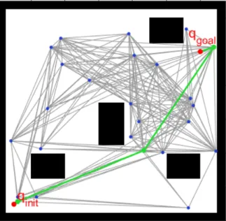
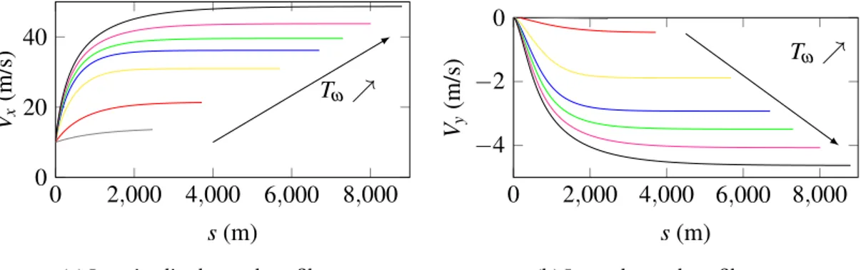
4.2 Example of trajectories obtained withδa= 1◦for different wheel torques Tωapplied. 69 4.3 Example of speed profiles obtained withδa = 1◦ for different wheel torques Tω applied. The colors matches with the trajectories displayed in Figure 4.2. . . 69
4.4 Curvature radius versus speed for different steering angles obtained with the 9 DoF vehicle model (full lines) and the kinematic bicycle model (dashed lines).. . . 69
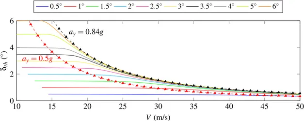
4.5 Theoretical kinematic steering angleδt hobtained by applying a steering angleδa on the 9DoF model (full line), and maximum kinematic steering angleδmax al-lowed for different maximum lateral accelerations aymax(triangles). . . 70
4.6 Lateral acceleration versus speed for different steering angles obtained with the simulation model.. . . 70
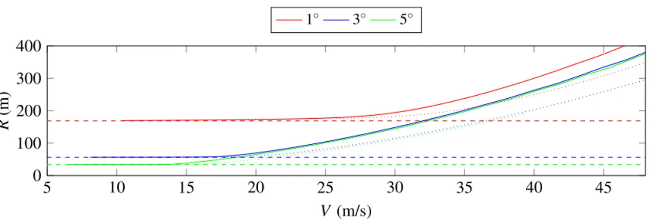
4.7 Radius versus speed for different steering angles obtained with the 9DoF model forµ = 0.7 (full lines), µ = 1 (dotted lines) and with the kinematic bicycle model (dashed lines). . . 71
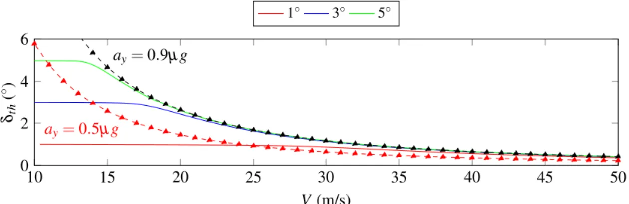
4.8 Theoretical kinematic steering angleδt hobtained by applying a steering angleδa on the 9DoF model withµ = 0.7 (full line), and maximum kinematic steering angle δmaxallowed for different maximum lateral accelerations aymax(triangles).. . . 72
4.9 Validity of the kinematic bicycle model. . . 72
4.10 The planning and control architecture proposed. . . 73
4.11 Parabola defined by the obstacle manager. . . 74
4.12 Reference track. The obstacles are in red. The numbers indicate different road sections to facilitate the matching with Figures 4.14 and 4.17. . . 78
4.13 Trajectories planned by MPC (green lines) and actual trajectory followed by the
controller (blue dots), with obstacles (red dots). . . 78
4.14 Comparison between Vheur(red), Vr(green) and V (blue), in the case of no obstacles. 79 4.15 Longitudinal slip ratio at each wheel in the case of no obstacles. . . 79
4.16 Lateral slip angle at each wheel in the case of no obstacles. . . 79
4.17 Total steering angleδ (blue) and closed-loop steering angle δf b(green): (a) without obstacles; (b) with obstacles. . . 79
4.18 Wheel torque applied on the front left wheel: without obstacles (blue); with obsta-cles (red). . . 80
4.19 Absolute value of the lateral error in the case of no obstacles. . . 80
4.20 Computational time in the case of no obstacle (blue) and with obstacles (red). . . . 80
4.21 Trajectories planned by MPC (green lines) and actual trajectory followed by the controller (blue dots), with obstacles (red dots). The numbers indicate different road sections to facilitate the matching with Figures 4.17 and 4.22. . . 81
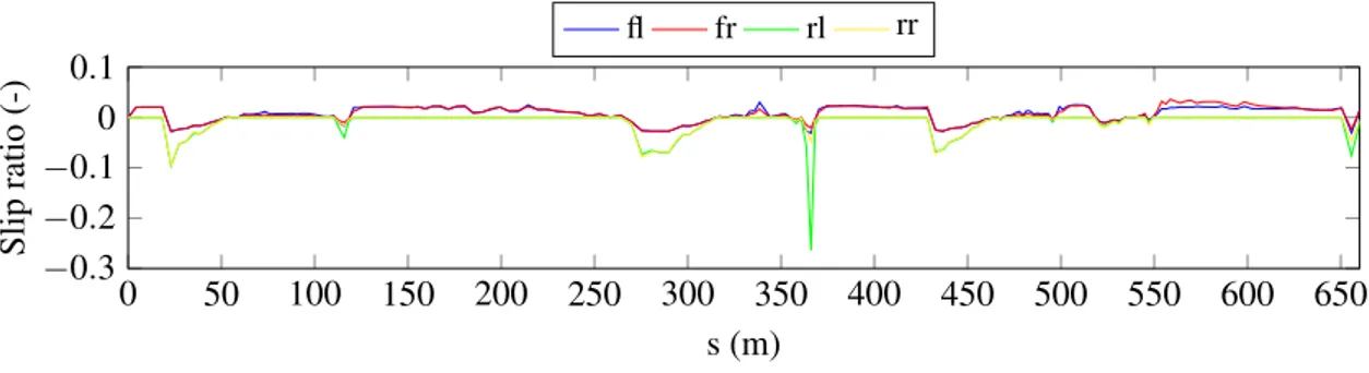
4.22 Comparison between Vheur (red), Vr (green) and V (blue), in the case of obstacles. 81 4.23 Longitudinal slip ratio at each wheel in the case of obstacles. . . 82
4.24 Lateral slip angle at each wheel in the case of obstacles. . . 82
4.25 Heuristic speed (red), reference speed computed by the MPC (green) and actual speed of the vehicle (blue) for (a) wet roads (µ = 0.7) and (b) icy roads (µ = 0.2). . . 85
4.26 Steering angle inputs: (a) on wet road (µ = 0.7) and (b) on icy road (µ = 0.2). . . 85
4.27 Slip ratios (a) and slip angles (b) at each wheel on wet road (µ = 0.7): front-left (blue), front-right (red), rear-left (yellow) and rear-right (green). . . 86
4.28 Slip ratios (a) and slip angles (b) at each wheel on icy road (µ = 0.2): front-left (blue), front-right (red), rear-left (yellow) and rear-right (green). . . 86
5.1 PI controller with anti-windup. . . 94
5.2 The bicycle model: the two front (resp. rear) wheels (in grey) are lumped into a unique wheel (in black). . . 95
5.3 PID controller. . . 96
5.4 Pure-pursuit controller. . . 97
5.5 Stanley controller. . . 98
5.6 Frenet frame for the kinematic bicycle model. . . 99
5.8 The lateral displacement. . . 104
5.9 The pseudo distance. . . 105
5.10 Shanghai Jiao-Tong’s CyberGL8 vehicle used for experimentations.. . . 106
5.11 Reference path (in red) in the Shanghai Jiao-Tong University campus. . . 106
5.12 Preview distance of the pure-pursuit controller for different speeds. . . 107
5.13 Trajectories obtained with the different controllers. . . 109
5.14 Zoom on the sharp turn. . . 110
5.15 Zoom on the long turn. . . 110
5.16 Speed profiles of the vehicle for each controller. . . 111
5.17 Lateral error as a function of the curvilinear abscissa for each controller. . . 111
5.18 Distribution of the absolute value of the lateral error for each controller. . . 112
5.19 Heading angle error as a function of the curvilinear abscissa for each controller. . . 112
5.20 Distribution of the absolute value of the heading angle error for each controller.. . 113
5.21 Comparison of the steering angleδ for each controller. . . 113
5.22 Comparison of the steering angle obtained at the front wheel for each controller in the sharp turn. . . 114
5.23 Estimation of the curvatureκ of the reference path for the KBCF controller.. . . 114
5.24 Estimation of the derivative of the curvaturedd tκof the reference path for the KBCF controller. . . 114
6.2 Structure of the vehicle powertrain to be controlled. . . 128
6.3 Considered cascading control structure.. . . 128
6.4 Description of the brake system . . . 129
6.5 Open-loop response of the brakes. . . 129
6.6 Tuning of parameterα for the brake system in open-loop. . . 130
6.7 Feedforward response forα = 200 of the brake system. . . 130
6.8 Tuning of parameter KPfor the brake system (α = 800). . . 130
6.9 Comparison between PI and i-P controllers for the brake system . . . 131
6.10 Top view of the open road test field track. . . 132
6.11 Altitude of the track. . . 132
6.12 Tuning of theα parameter for the high-level controller.. . . 133
6.13 Response of the model-free controller for different values of KPandα = 0.008. . . . 133
6.14 Comparison of the speed profile between the i-P and PI controllers. . . 134
6.15 Lane change maneuver with a lateral MFC at V = 5m/s without (blue) and with 50ms actuation delays (green). The initial configuration of the vehicle is given in grey and KP= 5, KD= 6.47.. . . 135
6.16 Lateral error for a lane change maneuver with a lateral MFC at V = 5m/s without (blue) and with 50ms actuation delays (green) for KP= 5, KD= 6.47. . . 135
6.17 Steering angle for a lane change maneuver with a lateral MFC at V = 5m/s without (blue) and with 50ms actuation delays (green) for KP= 5, KD= 6.47. . . 135 A.1 Slip angle and notations. . . VII A.2 Top view of a four-wheel vehicle model. . . VIII
1.1 The different SAE levels. . . 9
2.7 Coefficients of LuGre model. . . 35
2.8 Coefficients of Burckhardt model. . . 36
4.3 Parameters of MPC.. . . 76
5.1 Influence of PID gains . . . 96
5.2 Comparison of the lateral errors (m). . . 111
5.3 Comparison of the angular errors (rad). . . 112
5.4 Summary of lateral controllers. . . 115
6.1 PID versus iPID controllers . . . 120
6.2 ALIEN filter coefficients for estimatingby.˙ . . . 123
6.3 ALIEN filter coefficients estimatingy.b¨ . . . 123
6.4 ALIEN filter coefficients for estimatingbF (ν = 1). . . 123
6.5 ALIEN filter coefficients for estimatingbF (ν = 2). . . 123
6.6 Model-free controller tuning guidelines. . . 125
6.7 Comparison of the root mean square of the tracking error between PI and i-P con-trollers. . . 134
This work would not have been possible without the direct or indirect contributions of many peo-ple. First of all, I would like to thank my two advisors: Brigitte, who has always guided me thor-oughfully in my research and read all my publications scrupulously, correcting even punctuation and accentuation errors; Arnaud, who trusted me even though I did not have a background in robotics/automation and encouraged me to nurture my knowledge on autonomous vehicles out-side of my domain. This work would not have been possible also without Florent, whose strong scientific and computer science skills guided me throughout my thesis, and Sébastien, from whom I got the chance to learn a lot on control applications and scientific rigor during my numerous stays in Valenciennes.
I would also like to thank my lab mates with whom I have spent my three years of PhD: Xavier who introduced me to new board games especially King of Tokyo; Daniele who brought Italy to our doorstep; Edgar who aroused my curiosity with his music instrument “Embodme" combining mathematics and AI; Eva and Jun with whom I won the Valeo Innovation Challenge 2016; Jean-Emmanuel, Arthur and Michelle for visiting China together; Amaury and Hassan for our runs in the Luxembourg garden on Thursday mornings; Cyril for joining as a goalkeeper my soccer team; Philippe for our passionate debates about politics and life; Guillaume for visiting Hawaii with me; Hugues, Martin and Paul for the numerous board games; Aubrey for making me discover the slack line; Grégoire for an introduction to the virtual reality world; Mathieu for the rock’n’roll; Marion for the classical music; Marin for the crazy driving with Reinforcement Learning; Thomas for his help in C++. Thank you also to my colleagues François, Fabien, Silvère, Simon, and of course Christine and Christophe who easen my administrative tasks.
During my thesis, I also got the chance to meet a lot of researchers who took some time to dis-cuss my work. I would like to thank in particular Michel for thorough disdis-cussion about model-free control, Eduardo about Model Predictive Control, Jean-Paul and Nicolas about motion planning, Lghani, Dominique, and people from the Chair, in particular Wei, Ching-Yao and Wei-Bin from UC Berkeley.
My three months in China have been quite of an adventure too! I have discovered a whole new culture with wonderful colleagues. In particular, I would like to thank Chaojie, mister “super out-standing", for showing me around and introducing me to the chinese culture; Wei, mister “sugar" (his lastname Tang means sugar in chinese), for helping me out with the administrative stuffs and driving me like an “old driver" to the airport; Lihong for his always positive energy; Yao for our controller contest.
I am very grateful to the jury members for assessing my work: Thierry-Marie whose nice com-ments about the manuscript persuaded me that it was worth spending a couple of months on this task; Philippe for his challenging comments about my work; Ming for his curiosity about my re-cent research on deep learning control and without whom my three-month experience in China would not have been possible; Alain for his course about PID control.
My family and friends have also played an important role in this work. In particular, I would like to thank my parents and my brother for their support, and my grand-mother for coming to my PhD defense all the way from Le Mans at the age of 95!
Last but not least, I would like to gratefully thank Tan-Mai, who always gave me her support, not only in the good times but also in the harder moments during this thesis... This work would not have been possible without her constant encouragements!
The work undertaken during this thesis is part of the international research Chair MINES Paris-Tech - Peugeot-Citroën - Safran - Valeo on ground vehicle automation and coordinated by Profes-sor Arnaud de La Fortelle1. This research Chair also comprises academic partners: University of California Berkeley (USA), Ecole Polytechnique Fédérale de Lausanne (Switzerland) and Shanghai Jiao-Tong University (China).
This five-year Chair with a funding of 3.7 million euros has three main objectives: • Improve the knowledge on autonomous driving;
• Develop onboard intelligence devices;
• Run automated vehicle tests on three different continents (Asia, North America and Europe).
Introduction
“ Si l’on se préoccupait de
l’achèvement des choses, on n’entreprendrait jamais riena”
aIf we were concerned about the
completion of things, we would never undertake anything
François Ier, roi de France
Contents
1.1 What is an autonomous vehicle? . . . . 6
1.1.1 History of autonomous vehicles . . . 6
1.1.2 From Advanced Driver Assistance Systems... . . 8
1.1.3 ... to fully autonomous vehicles. . . 9
1.2 Technical components of an autonomous vehicle . . . 10
1.2.1 Sense-Model-Plan-Act and the different robotic paradigms . . . 11
1.2.2 High-level cognitive tasks . . . 12
1.2.3 Low-level cognitive tasks . . . 12
1.3 Scope of the thesis . . . 13
1.3.1 Main assumptions . . . 13
1.3.2 Some important notions. . . 14
1.3.3 Consistency of the architecture. . . 15
1.1 What is an autonomous vehicle?
In 1886, Karl Benz patented the first motor vehicle in the world. He benefitted from the techno-logical advances entailed by the industrial revolution to make a vehicle move on its “own", based on an internal combustion engine, replacing progressively animal-drawn carriages. Interestingly, the french language distinguishes automobiles (motor vehicles) that are moving using their own energy from hippomobiles (carriages), horse-drawn vehicles [Laurgeau, 2009]. In less than half a century, motor vehicles completely changed the way people moved, destroying on its rise lots of jobs such as farriers to replace them by new ones, for example gas station attendants. Motor ve-hicles became accessible to the masses in 1908 with Ford’s Model T and became a symbol of the “American way of life" after World War II.
Nowadays, the digital revolution has replaced the industrial revolution, and in this “Second Machine Age" [Brynjolfsson and McAfee, 2014], the future of mobility might be completely re-shaped: the car which was seen in the 1980s as a purely mechanical object is now becoming more of an electronic device. And autonomous vehicles that might have been seen as pure science fic-tion until not so long ago are about to become real. This paradigm shift has some important con-sequences on the automotive industry market as clients are becoming more interested in digital features (ex: connectivity, driver assistance systems) than in mechanical performances (ex: horse-powers, acceleration capacities).
1.1.1 History of autonomous vehicles
The early stages of autonomous vehicle with actual vehicle prototypes date back to the 1980s, with mainly three projects:
• NavLAB – National Autonomous Vehicle LABoratory – launched in 1984 at Carnegie Mel-lon University [Thorpe et al., 1991a,Thorpe et al., 1991b] which proposed successive epony-mous vehicle prototypes: Navlab 1 in 1986 to Navlab 10 in 1996.
• Prometheus – PROgraM for a European Traffic of Highest Efficiency and Unprecedented Safety – a European project promoted by Ernst Dickermanns at the Bundeswehr University of Munich and Mercedes-Benz, launched in 1987, and which led to a prototype, the VaMP (Versuchsfahrzeug für autonome Mobilität und Rechnersehen1).
• California PATH – Partners for Advanced Transit and Highways – program founded in 1986 [Shladover, 2006] as a collaboration between California Department of Transportation (Cal-trans), UC Berkeley and other public and private partners, and which has been a pioneer in Automated Highway Systems (AHS), in particular focusing on increasing the highway ca-pacity and safety while reducing the traffic congestion, the air pollution and the energy con-sumption.
However, already back in 1925, the inventor Francis Houdina and his company Houdina Radio Control demonstrated a radio-controlled “driverless" car, the American Wonder, nicknamed the “Phantom Auto", which drove on Broadway and Fifth Avenue in New York without any human on-board2. It was controlled remotely by a human located in a second car following close behind using radio technology.
Many other projects have emerged afterwards from the 1990s until now, such as the ARGO project3 (1996) led by the universities of Parma and Pavia in Italy, and the European projects
1Experimental vehicle for autonomous mobility and computer vision
2
https://www.inverse.com/article/14438-remotely-controlled-autonomous-vehicles-are-coming-for-better-or-for-worse, visited April 2018.
CityMobil4(2006-2011), CityMobil25(2012-2016), interactIVe6(2010-2013), AutoNET20307 (2013-2016), i-GAME8(2013-2016), iTeam9(2016-2019).
Research on Autonomous Vehicles really reached a milestone with the successive DARPA chal-lenges, organized by the Defense Advanced Research Projects Agency part of the United States Department of Defense. These challenges were the first long distance competitions for driverless car in the world. After a first unsuccessfull edition in 2004, the 2005 DARPA Grand Challenge was won by the Stanley vehicle from Stanford University (see Figure1.1a): it accomplished the 240km of route in the desert in 6 hours and 54 minutes. The 2007 DARPA Urban Challenge consisted in a 96km urban area course where the autonomous vehicles had to obey traffic rules, respect other traffic participants, and avoid obstacles. This time, the Boss vehicle from Carnegie Mellon Univer-sity won the competition at an average speed of 22.53km/h (see Figure1.1b).
(a) Stanley from Stanford University (b) Boss from Carnegie Mellon University
Figure 1.1 – The winners of the DARPA Grand Challenge in 2005 (a) and the DARPA Urban Challenge in 2007 (b).
More recently, other competitions took place. Among others, let’s mention:
• the Intelligent Vehicles Future Challenge (IVFC) which has been held every year in China since 2009 and gathers teams from many major universities and scientific research institu-tions of the country. The competitors are required to finish not only a test on an actual road in order to examine the safety, comfort, agility and intelligence of the driverless vehicle, but also an offline test to check out the vehicles’ basic cognitive ability by simulating an actual road environment.
• the Grand Cooperative Driving Challenges (GCDC) which were held in the Netherlands in 2011 [Ploeg et al., 2012] and in 2016 [Englund et al., 2016] and organized by the European project i-GAME. Their goal was to prove a basis for cooperative automated driving in an international context.
Some recent projects have confirmed the technical advances that have been made in the do-main of autonomous vehicles: in 2010, VisLab Intercontinental Autonomous Challenge (VIAC) in-volved four driverless vehicles which drove an almost 16000km trip from Parma in Italy, to Shang-hai in China. This challenge enabled to collect about 50 terabytes of data. Then in 2012, only 125 years after Karl Benz’s wife Bertha complete the first journey in automotive history, a vehicle from Daimler in collaboration with Karlsruhe Institute of Technology and Forschungszentrum In-formatik10completed the same journey from Mannheim to Pforzheim in fully autonomous mode [Ziegler et al., 2014b]. Finally, the Google car project11 launched in 2009, is probably the project
4http://www.citymobil-project.eu/, visited on December 2017. 5http://www.citymobil2.eu/en/, visited on December 2017. 6http://www.interactive-ip.eu/, visited on December 2017. 7http://www.autonet2030.eu/, visited on December 2017. 8http://gcdc.net/en/i-game, visited on December 2017. 9https://iteam-project.net/, visited on December 2017. 10Research Center for Information Technology
that has gained most public attention. In February 2018, its fleet of vehicles had drove over 5 mil-lion miles12 in self-driving mode, with a rate growing exponentially due to the expansion of the number of vehicles. In December 2016, Google decide to launch a subsidiary company, named Waymo, working specifically on autonomous vehicles. Other companies, such as Uber or NuTon-omy have also launched a huge fleet of vehicles around the globe to test their technology. Notice that France has also some companies with their own fleet, such as Navya and Easymile.
1.1.2 From Advanced Driver Assistance Systems...
Safety has always been the main priority for both the car industry and legislators. Car accidents are responsible for over 3400 deaths and 70000 casualties in 2017 in France13, 37000 deaths and 2000000 casualties in 2016 in the USA14, and 1.2M deaths worldwide15in 2013. To reduce these figures, the automotive industry has been developing constantly new safety systems. Commonly, we distinguish passive and active safety systems:
• Passive safety is used to refer to components of the vehicle that help to protect occupants during a crash.
Examples: airbags, seatbelts and the physical structure of the vehicle.
• Active safety is used to refer to technology assisting in the prevention of a crash.
Examples: Anti-lock Braking System (ABS), Electronic Stability Program (ESP) and Advanced Driver Assistance Systems (ADAS).
First, research on active safety has been focusing on how to enhance the handling and stability of the vehicle, by compensating some undesired dynamic effects. They have lead to the develop-ment of new systems, in particular:
• Anti-lock Braking System (ABS) - 1978: braking assist system that prevents the wheels from locking up during severe braking.
• Electronic Stability Program (ESP) - 1995: antiskid system aimed at enhancing the control of the vehicle for a better road handling. It enables to detect the loss of grip in curves and counteract by braking one or several wheels.
These systems are now mandatory on all new vehicles in the European Union since respectively 2004 and 2014.
However 94% of car accidents are due to human factors16, such as drowsiness, alcohol and speeding. Therefore with the emergence of technologies for autonomous vehicles, car manufac-turers and Original Equipment Manufacmanufac-turers (OEM) have developed increasingly efficient active safety systems, such that nowadays, the driver can be relegated to a role of simple supervisor of the driving task; the onboard intelligence is able to act directly on the steering, acceleration and brak-ing. These systems, gathered under the acronym ADAS (for Advanced Driver Assistance Systems) are already available on high-end commercial vehicles. Among them, let’s mention:
• Adaptive Cruise Control (ACC) - 2011: cruise control system that automatically adjusts the speed of the vehicle to maintain a safe distance with the preceding one.
• Collision Avoidance System or Autonomous Emergency Braking (AEB) : system that either provides a warning to the driver when there is an imminent collision risk or takes action autonomously, generally by braking at low vehicle speeds (below 50 km/h) and by steering at higher speeds.
12https://waymo.com/ontheroad/, visited on April 2018.
13
http://www.securite-routiere.gouv.fr/la-securite-routiere/l-observatoire-national-interministeriel-de-la-securite-routiere, visited on April 2018.
14https://www.nhtsa.gov/press-releases/usdot-releases-2016-fatal-traffic-crash-data, visited on April 2018. 15http://www.who.int/gho/road_safety/mortality/traffic_deaths_number/en/, visited on April 2018. 16https://crashstats.nhtsa.dot.gov/Api/Public/ViewPublication/812115, visited on April 2018.
• Lane-Departure Warning (LDW) - 1992: system that warns the driver when the vehicle be-gins to move out of its lane (unless the turn signal is on in that direction).
• Lane Keeping System (LKS) : feature that in addition to the lane departure warning system automatically takes actions to ensure the vehicle stays in its lane.
• Park Assist: system that moves automatically a vehicle from a traffic lane into a parking spot by performing parallel, perpendicular or angle parking.
Finally, eCall launched by the European Union and mandatory since April 2018 on all new vehicles enables to automatically send an emergency call in the case of a crash providing its precise localization and its severity.
1.1.3 ... to fully autonomous vehicles
The automation of a vehicle has been classified into 6 different levels by the Society of Automotive Engineers17(SAE). These levels are summarized in Table1.1, starting from level 0 corresponding to no automation to level 5 where the steering wheel and pedals are not necessary anymore. These levels are now standard in the car industry since their adoption by the National Highway Traffic Safety Administration (NHTSA), part of the United States Department of Transportation.
N◦ SAE Levels Description
0 No Automation
The full-time performance by the human driver of all as-pects of the dynamic driving task, even when enhanced by warning or intervention systems.
1 Driver Assistance
The driving mode-specific execution by a driver assis-tance system of either steering or acceleration/deceler-ation using informacceleration/deceler-ation about the driving environment and with the expectation that the human driver performs all remaining aspects of the dynamic driving task.
2 Partial Automation
The driving mode-specific execution by one or more driver assistance systems of both steering and acceler-ation/ deceleration using information about the driving environment and with the expectation that the human driver performs all remaining aspects of the dynamic driving task.
3 Conditional Automation
The driving mode-specific performance by an Auto-mated Driving System of all aspects of the dynamic driv-ing task with the expectation that the human driver will respond appropriately to a request to intervene.
4 High Automation
The driving mode-specific performance by an Auto-mated Driving System of all aspects of the dynamic driv-ing task, even if a human driver does not respond appro-priately to a request to intervene.
5 Full Automation
The full-time performance by an Automated Driving Sys-tem of all aspects of the dynamic driving task under all roadway and environmental conditions that can be man-aged by a human driver.
Table 1.1 – The different SAE levels.
17
Combining different ADAS presented in section1.1.2can provide vehicles up to level 2. This is the case for example of Tesla Motors’ vehicles where the different assistance systems are gathered under the name “Autopilot”. The vehicle is able to remain in its lane while adjusting its speed to the vehicle located in front. However, such vehicles are not autonomous vehicles as the driver might have to take over the control at anytime due for example to snow conditions hidding the lane marking18or unclear lane marking19. Today, only commercial vehicles up to level 2 are available on the market and allowed to drive on public roads. Audi has announced the release of the first commercial vehicle of level 3 by 2019: the Audi A8. But according to Vienna Convention (1968), the driver remains responsible in the case of an accident.
Nowadays most carmakers and OEM have their own autonomous vehicle prototypes, some-times up to level 4, pushed by disruptive actors stemming from the technological area such as Google, Tesla, Uber and even Apple. The prototype of the Valeo’s hands-off tour is displayed as an example in Figure1.2and the Google car in Figure1.3. However, these vehicles have often a very conservative driving strategy. Therefore, they can be unefficient in terms of traffic flow as they can get stuck by for example road works, stopped cars, traffic wardens or four-way stops. In particular, they are unable to take a decision when there is too much uncertainties20. Moreover, they often rely on a human intervention to perform a lane change (or at least to take the decision).
Figure 1.2 – Valeo’s hand-off tour prototype.
Figure 1.3 – The Google Car.
1.2 Technical components of an autonomous vehicle
An autonomous vehicle is a wheeled robot. The hardware and software used in the early stages of autonomous vehicles were simple adaptation of the one used on small wheeled robots. These al-gorithms were suited for the low speed applications considered at the beginning, where dynamics effects for example could be neglected, as the goal was to build a Proof of Concept. As a robot, the
18https://www.youtube.com/watch?v=lTtLGP4cRaQ, visited on April 2018.
19https://www.youtube.com/watch?v=6QCF8tVqM3I&feature=youtu.be, visited on April 2018. 20https://www.youtube.com/watch?v=tiwVMrTLUWg, visited on April 2018.
organization of an autonomous vehicle can be divided into tasks that require more or less intelli-gence.
1.2.1 Sense-Model-Plan-Act and the different robotic paradigms
Like any system provided with Artificial Intelligence (AI), an autonomous vehicle relies on the four primitives of robotics presented in Table1.2:
Sense
Gathers information from different sensors on the state of the robot and its sur-roundings. There exist two types of sensors: proprioceptive sensors which measure the internal state of the robot such as Inertial Measurement Units (IMU) and wheel encoders, and exteroceptive sensors which acquire information from the robot’s en-vironment like Global Positioning Systems (GPS), cameras, LIght Detection And Ranging (LIDAR) or RAdio Detection And Ranging (RADAR).
Model
Creates a world model from the sensor information, in order to determine (i) the position of the robot using Simulatenous Localization And Mapping (SLAM), (ii) the free-space where the robot can move and (iii) the intention of the dynamic ob-stacles.
Plan
Determines a goal for the robot using navigation and/or a behavioral layer and computes a safe path/trajectory to follow in order to reach it. A path consists in a list of positions (Xi, Yi)i ∈1,nin the physical space while a trajectory is a path
in-dexed by time (or equivalently, with a velocity encoded). Act
Commands the actuators of the robot, namely the brake and gas pedals and the steering wheel in the case of an autonomous vehicle, in order to track the reference path/trajectory.
Table 1.2 – The four robotic primitives.
These primitives are organized according to a paradigm, defined as a philosophy or set of as-sumptions and/or techniques which characterizes an approach to a class of problems. There exist three main paradigms for robotic systems [Murphy, 2000]: the hierarchical paradigm, the reactive paradigm and the hybrid deliberative/reactive paradigm. Under the hierarchical paradigm, the robot performs at each step successively the Sense-Plan-Act tasks. The reactive paradigm relies on the Sense-Act tasks: the Plan task is relegated to the background, or even eliminated. There-fore, it has a faster execution time. Finally, the hybrid deliberative/reactive paradigm first performs the Plan task and then decomposes the planning goal into subtasks where the reactive paradigm Sense-Act is executed. The organization of the different paradigms are represented in Figure1.4.
(a) Reactive paradigm (b) Hierarchical paradigm (c) Hybrid deliberative/reactive paradigm
Figure 1.4 – The different robotic paradigms [Murphy, 2000].
Remark 1. Note that the primitive “Model" has been introduced only recently and is therefore not
1.2.2 High-level cognitive tasks
High-level cognitive tasks require some kind of “intelligence" in order to be performed: they con-sists in tasks that humans are good at and that cannot be easily translated into algorithms.
Perception
Perception, which corresponds to the SENSE primitive of a robot, is very critical for the safety of an automous vehicle. It is responsible for gathering all the necessary information on the driving scene, i.e. the position and nature of the obstacles, the traffic signs, the drivable road corridors... This task is rather easy for a human but much harder for a computer as it requires to understand the scene, in particular its semantic: for example, to tell the difference between a biker and a pedestrian. As mentioned previously, it comprises proprioceptive and exteroceptive sensors. Usu-ally, autonomous vehicles are equipped with four wheel encoders, one per wheel, to compute the rotational speed of each wheel; an IMU to get the three angular and three linear accelerations of the vehicle; a GPS to receive its position in the inertial coordinate system; one or several cameras to detect the lane marking, pedestrians, vehicles, traffic signs and other sementic information in the scene; one or several LIDARs and/or RADARs to obtain the distances to static and dynamic objets; ultrasounds for parking and tight maneuvers.
Simultaneous Localization And Mapping (SLAM)
After collecting information on the environment, the vehicle needs to build a local map of the scene, to understand where it is allowed to drive, what the other traffic participants are doing, and to localize itself accurately in the scene. This is done using Simultaneous Localization And Mapping (SLAM). These algorithms have been widely developed by the robotics community (see [Cadena et al., 2016] for a review of the different techniques). As the name indicates, they enable to localize the vehicle while creating a map of the environment, i.e. the roads, the static and dynamic obstacles. One of the main difficulty of such algorithms applied to autonomous vehicles compared to conventional robots is not only the large number of dynamic obstacles and thus of occlusions encountered, but also their higher velocities. Hence, SLAM requires to understand the semantic of the scene such as where is the vehicle allowed to drive and occlusions. It is thus a hard task for a computer.
Decision-making and planning
Finally, an autonomous vehicle needs to have a goal and plan how to get there. While the navi-gation task precomputes the route to get to the final destination, it is still necessary to compute local plans during the travel in order to perform lane change maneuvers (either to overtake a slow vehicle located in front or to take an exit on the highway), merging into a lane with other traffic participants, crossing a four-way stop and other similar actions. These maneuvers require a lot of decisions such as when it should do it and how, and thus a certain risk. Evaluating the risk can be rather difficult sometimes for a computer as it implies social behavior too and trade-off between drivers.
1.2.3 Low-level cognitive tasks
Unlike high-level cognitive tasks, low-level ones do not require any specific intelligence. These tasks are relatively easy to implement on computers and provide better results than human. Such tasks are either repetitive (keeping a constant speed for example), require a great accuracy or lot of computation.
Observation and filtering
In order to keep the costs low, some internal states of the vehicle such as its speed cannot be directly measured. Instead, observers stemming from control theory are used (see for example Luenberger observers for linear systems [Luenberger, 1971]). They provide an estimation of the internal state from the measurements of the input and output signals of the system. Moreover, due to the low costs of the sensors such as the IMU, the quality of the measurements is usually poor. Therefore, filters are necessary. In particular, Kalman filters [Kalman and Bucy, 1961] en-able to improve the estimation of the internal states of the vehicle such as its localization or its velocity, despite model errors and measurement noises, by merging measurements provided by proprioceptive sensors such as the IMU with exteroceptive sensors such as the GPS.
Control and tracking
Controllers are ubiquitous in modern vehicles, in particular in autonomous one. They correspond to the ACT primitive. Their objective is to provide an input signal to the system, also referred to as a control law, in order to track a desired reference output while ensuring the stability of the system. They are used for example for generating the throttle to maintain a constant speed dur-ing cruise control, as well as for the different ADAS presented in section1.1.2. Control laws are often simple to implement on a computer, in particular if a closed-loop form can be found, and are outperforming a human to track a reference signal. While the stability and the accuracy of the tracking are usually the most important criteria, some other ones can be considered too such as the smoothness of the control input, the time response or overshoots.
Observability and controllability are two dual concepts in control theory that are important in order to obtain a desired result. While adding new sensors to the system might improve its observ-ability, adding new actuators might improve its controllability. In the case of autonomous vehicles, the actuators are the gas pedal, the brake pedal and the steering wheel, even though some systems such as the ESP can provide a differential torque to the wheels to improve the controllability of the vehicle. However, in some cases the system becomes not controllable: for example, during gear shift, the torque generated by the engine is not transmitted to the wheel as the clutch is opened. While this case is relatively non important regarding the vehicle safety, other cases are much more critical such as slip and skid, where the vehicle can loose control (the steering wheel has no impact on the direction of the vehicle anymore). These cases need to be avoided and will be explained in chapter2.
1.3 Scope of the thesis
1.3.1 Main assumptionsThis thesis deals with autonomous vehicles. Throughout this work, a vehicle will be said to be au-tonomous if it compels with the levels 4 or 5 defined by the SAE standards. In the literature, see for example [Qian et al., 2017], some authors distinguish an autonomous vehicle from a coopera-tive vehicle: in the first case, the vehicle relies solely on its own sensors while in the second case, the vehicle also gets information from other vehicles and the infrastructure, through respectively Vehicle-to-Vehicle (V2V) and Vehicle-to-Infrastructure (V2I) communications. Such a distinction will not be made in this work. Therefore, an autonomous vehicle can rely both on its own sensors or on communication.
As research on autonomous vehicles is getting more and more mature, the question of consis-tency between its different layers, namely perception (SENSE), localization and mapping (MODEL), motion planning (PLAN) and control (ACT), is becoming crucial to ensure the safety of the vehicle at all time. An ill-designed vehicle architecture might be very critical for its safety, even though each layer is well-designed independently. Our work focuses on the Plan-Act primitives defined
in section1.2.1, which will be referred to as respectively the motion planning and the low-level control tasks, in order to define a “good" motion planning and control architecture. Therefore, we assume that (i) all the information needed to take a decision is known (the environment is fully observable), (ii) the world model is known and given as input of the planning layer, (iii) a naviga-tion task or a behavioral layer provides a goal to the vehicle. More precisely, the inputs comprise a map with the coordinates of the road centerlane and its boundaries, the reference lane assigned by the navigation task, and the position and velocity of all the obstacles. The detection of obstacles will not be considered at any stage during this work.
1.3.2 Some important notions Control
The word control refers to the fact of bringing a system to a desired state by acting on its inputs. In control theory, it is common to consider single input single output (SISO) systems and to derive a closed-loop form for the control signal where stability proofs for the system can be demonstrated. In the robotic community, the large number of degrees of freedom and/or actuators compels to use “optimal control" formulation in order to find a solution, i.e. an optimization problem where the goal is to minimize/maximize a criterion while respecting some constraints on the system.
Feasibility
The word feasibility will play a major role in this work but its meaning is ambiguous and depends on the context. It is defined as “capable of being done or carried out"21. Among the motion plan-ning community, people claim that their stated problem is feasible if there exists a mathematical solution: this means that there exists a collision-free path or trajectory between two configura-tions for example. This will be referred to as the mathematical feasibility. However, the solution obtained might not be feasible, this time in the physical sense, because it does not respect some laws of motion of the vehicle. This problem arises for example if the vehicle model used in the motion planning problem is not adapted to the situation. This will be referred to as the dynamic feasibility.
Consistency
The word consistency is probably the most important one in this thesis, or more precisely its antonym inconsistency. The Merriam-Webster Dictionary22defines the later as the quality or state of being: (i) not compatible with another fact or claim; (ii) containing incompatible elements; (iii) incoherent or illogical in thought or actions.
Inconsistency problems between the motion planning and control layers may arise due to some assumption mismatches, corresponding to definition (i) or (ii): for example, it is common to assume that the reference trajectory provided to the controller is C2in order to have a continuous curvature. However, if no precaution is taken, the motion planning has no reasons to deliver a trajectory with such properties (not even continuous)! However, we will focus on definition (iii) in this work: choosing an improper level of modeling when defining a motion planning or control problem might lead to some illogical actions.
Model
A model is a mathematical representation of a real world system. It enables not only to describe and understand its behavior but also to predict its evolution. Models play a fundamental role in a large variety of robotic applications such as simulation, control theory, motion planning or pre-diction intention. However, a model for a given system is neither unique nor universal. It is a
21https://www.merriam-webster.com/dictionary/feasible, visited on April 2018. 22https://www.merriam-webster.com/dictionary/inconsistent, visited on April 2018.
trade-off between conflicting objectives: the computational efficiency to solve it, its accuracy, its validity and the a priori knowledge of the system. One particularity about models is that they can be true but irrelevant for some applications, either because they are too complex for the applica-tion considered or because they do not model certain phenomena that cannot be neglected in this case. Therefore, defining a proper model [Ersal et al., 2008] is not straightforward and depends on the level of abstraction of the problem considered. Thus, when a model is used, it is important to have in mind the underlying assumptions that have been made. Otherwise, the mismatch with re-ality can be huge. Using a model that is consistent with the problem considered is therefore critical for the safety of the vehicle. In a sense, a model is like a drawing: the more details are included, the longer it takes to execute it.
1.3.3 Consistency of the architecture
In her inaugural lecture on “Algorithms" at College de France23, Claire Mathieu underlines that an algorithm might lead to bad solutions not because the resolution is wrong but because the stated problem is not relevant or well-posed. In the case of an autonomous vehicle, such a problem may arise in the motion planning and control architecture due to inconsistencies. They can be found at three different levels: at the planning level, due to an improper level of modeling of the vehicle dynamics; at the control level, as its operational domain must be able to track at least all planned trajectories from the motion planner and also be robust to noise and disturbances; at the junction between the motion planning and control layers, due to some assumption mismatches between the two layers, such as the continuity or smoothness of the planned trajectory.
Motion planning and control problems are two different but highly related problems. The first one consists in computing a dynamically feasible trajectory for the vehicle, avoiding the surround-ing obstacles such as other vehicles, pedestrians, or non movsurround-ing objects. The second is actsurround-ing on the actuators, i.e. the gas pedal, brake pedal and steering wheel, in order to track the trajectory ob-tained by the motion planner, while ensuring the stability of the system and, if possible, a smooth drive. Therefore, the properties of the design of each layer are quite different.
At the motion planning layer, the algorithm is searching a trajectory that respects some safety and comfort constraints while optimizing some criteria. Such a search is computationally expen-sive and requires therefore both a simple model of the vehicle and a low computational frequency (around 5-10Hz). On the contrary, control usually operates at high-frequency (around 100Hz) to ensure a good tracking of the reference trajectory. Moreover, the level of abstraction of the mo-tion planning and the control layers also differs. For example, dealing with obstacles is one of the main task of the motion planner while the controller usually completely ignores them: the tra-jectory given by the motion planner is assumed to be safe within a certain margin and the goal of the controller is then to follow as well as possible the given trajectory, without considering the obstacles.
In most studies the low-level control is not considered at the motion planning phase; in-stead, the general assumption is that, provided the planned trajectory satisfies a certain set of constraints, the low-level control will be able to track this trajectory with a bounded error. In some actual implementations, the low-level controller is provided by the OEM’s test car as a black-box, with hard limits on the acceptable inputs of this control to prevent the vehicle from leaving its handling envelope. Such “black-box” behavior effectively fully isolates motion planning and con-trol.
Conversely, research on low-level vehicle control often assumes that a predefined reference trajectory is known in advance and does not change over time. However, due to the presence of dynamic obstacles on the road, notably other traffic participants, this assumption is in general untrue.
23https://www.college-de-france.fr/site/claire-mathieu/inaugural-lecture-2017-11-16-18h00.
1.4 Contributions
In this thesis, we claim that the intention of the motion planner, expressed as the future trajectory of the vehicle, should match with the one actually executed by the low-level controllers.
In other words, the motion planning and control architecture should be consistent as defined previously by choosing proper models and studying the influence of the interaction between the two layers on the overall performance.
Therefore, we will investigate some fundamental questions concerning the safety of an au-tonomous vehicle, in particular on the guarantees that can be obtained. This starts at the motion planning level by answering the following question:
Question 1: Can we guarantee the kinematic and dynamic feasiblity of a trajectory computed by the motion planner?
Therefore, after a reminder about vehicle dynamics and modeling in chapter2and a review of state-of-the-art motion planning methods in chapter3, chapter4deals with the question of con-sistency of the model used to plan a feasible trajectory avoiding obstacles while driving the vehicle towards its goal. In fact, the motion planner proposed is based on a kinematic bicycle model.
The second part of this thesis will focus on low-level control problems, stemming from con-trol theory. As such, the algorithms described therein are not specific to an autonomous vehicle but can be used in the design of some ADAS such as an ACC or a LKS. Many longitudinal and lat-eral controllers have been proposed in the literature for such purposes. However, these controllers have an operational limit: thus, chapter5will recall some of the commonly used lateral controllers and answer the following critical question regarding safety:
Question 2: Given a reference trajectory, can we ensure the performance of a lateral controller?
Finally, the last part of this thesis will focus on a newly introduced model-free control paradigm, proposed by [Fliess and Join, 2013], and its application to vehicle control. Due to the complexity of vehicle dynamics, in particular of tire dynamics, and the large number of parameters that not only vary from one situation to another but also are difficult to estimate, the model-free control appears as a promising solution. One reason therefore is that it estimates in real-time the dynam-ics of the vehicle. However, the following questions need to be addressed:
Question 3: How to implement model-free controllers on an autonomous vehicle? And what guarantees can we have on the results?
We will try to give an answer to these questions in chapter6. This chapter is completely inde-pendent from the rest of this thesis.
Vehicle dynamics and motion modeling
“ A theory has only the alternative
of being right or wrong.
A model has a third possibility: it may be right, but irrelevant ”
Manfred Eigen
Contents
2.1 Carbody dynamics - the slow dynamics . . . 23 2.1.1 Dynamic bicycle model . . . 23
2.1.2 Four-wheel vehicle model . . . 24 2.2 Tire dynamics - the fast dynamics . . . 26 2.2.1 Pacejka’s Magic Formula. . . 29
2.2.2 The linear tire model . . . 33
2.2.3 Dugoff model . . . 34
2.2.4 Other models . . . 35 2.3 Vehicle simulator . . . 37 2.3.1 The simulator engine. . . 37
2.3.2 The graphical interface - coupling to PreScan . . . 39 2.4 Simplified models for motion planning and control . . . 41 2.4.1 The point-mass model . . . 41
2.4.2 The unicycle model. . . 41
2.4.3 The kinematic bicycle model . . . 42
A physical system can be represented by a wide range of models, each one having some as-sets and drawbacks. The choice of a model is usually a trade-off between its accuracy, its com-putational efficiency, its robustness to modeling errors or uncertain parameters, and the level of abstraction necessary. The more detailed the model is, the more computational time is needed to solve it. Moreover, more details often require more information about the system: therefore, if only a few vehicle parameters are known, a complex model that requires a lot of information about the vehicle might be inappropriate, in particular if the model is not very robust to parameter un-certainties. Conversely, a detailed model can capture some phenomena that should be taken into account in certain situations, for instance slip and skid in the case of an autonomous vehicle.
In this chapter, we are interested in developing a high-fidelity vehicle simulator for testing our motion planning and control algorithms. The model used in the simulator needs to be as accurate as possible, taking into account phenomena such as slip or skid. The computational time is not the main issue and we suppose that we know all the information necessary about the vehicle. Therefore, a review of the different dynamic models which are the only models that comprise slip and skid are presented in a first time. The dynamics of a vehicle can be decomposed into two parts: a slowly-evolving dynamic (characteristic time of 0.1s to 1s) corresponding to the movement of the carbody and a fast dynamic (characteristic time of 1 to 10ms) corresponding to the movement of the wheels/tires. They will be presented respectively in secion2.1and2.2. Section2.3presents the vehicle simulator we have derived from the dynamic models and that will be used in the next chapters. Finally, section2.4introduces some simpler models that are used for motion planning and control.
Most of the explanations given in this chapter as well as complementary informations on vehi-cle dynamics can be found in [Rajamani, 2012,Kiencke and Nielsen, 2005,Gillespie, 1997]. All the main notations are given in Tables2.1,2.2,2.3,2.4,2.5and2.6. Figures2.1and2.2show the three different frames that will be used in the rest of this chapter: the inertial frame (~eX,~eY,~eZ) associated to the ground, the vehicle frame (~ex,~ey,~ez) and the pneumatic/tire frame (~pxi,~pyi,~pzi) associated
to each wheel i = 1..4.
Figure 2.2 – Vehicle frame (~ex,~ey,~ez) and pneumatic frame (~pxi,~pyi,~pzi) for each wheel i = 1..4.
Variables Meaning
MT Total mass of the vehicle MS Suspended mass of the vehicle
Ix, Iy, Iz Inertia of the vehicle around its roll, pitch and yaw axis
lf, lr Distance between the front (resp. rear) axle and the center of
gravity
lw Half-track of the vehicle
hCoG Height of the center of gravity of the vehicle
Table 2.1 – Notations for vehicle parameters. Variables Meaning
X, Y Position of the center of gravity of the vehicle in the inertial frame (~eX,~eY,~eZ)
θ, φ, ψ Roll, pitch and yaw angles of the carbody
Vx, Vy, Vz Longitudinal, lateral and vertical speed of the vehicle in its own
frame (~ex,~ey,~ez)
β Slip angle of the vehicle at center of gravity
δf Steering angle of the wheels located on the front axle
δf Steering angle of the wheels located on the rear axle
Tωi Total torque applied to wheel i
Tmi Motor torque applied to wheel i
Tbi Brake torque applied to wheel i
Tt ot Total torque applied to all the wheels
Table 2.2 – Notations for states and inputs of the vehicle. Variables Meaning
µ Friction coefficient of the road
µc Coulomb friction coefficient of the road
µs Static friction coefficient of the road
px, py Slope and road-bank angle of the road
Variables Meaning
Ir Inertia of the wheel
mr Mass of the wheel
rst at Radius of the wheel when the vehicle is static
r0 Radius of the wheel without any load re f f Effective radius of the wheel
ωi Angular velocity of the wheel i
Vxpi Longitudinal speed of the center of rotation of wheel i
ex-pressed in the tire frame (~pxi,~pyi,~pzi)
τxi Longitudinal slip ratio at wheel i
αi Slip angle at wheel i
τt ot al Total (longitudinal+ lateral) slip ratio at a wheel
γ Camber angle
Table 2.4 – Notations for states and characteristics of the wheels.
Variables Meaning
Fxpi, Fy pi Longitudinal and lateral tire forces generated by the road on the
wheel i expressed in the tire frame (~pxi,~pyi,~pzi)
Fxi, Fyi Longitudinal and lateral tire forces generated by the road on the
wheel i expressed in the vehicle frame (~ex,~ey,~ez)
Fzi Normal reaction forces on wheel i
∆Fsi Additional spring force of the suspension of wheel i compared
to the situation where the suspended carbody is at equilibrium Faer o Aerodynamic drag forces applied on the vehicle
g Gravitational constant
Table 2.5 – Notations for forces and torques.
Variables Meaning
zt i Heigth of wheel i in the inertial frame
zsi Heigth of the suspension of wheel i in the inertial frame
zr i Heigth of the road at wheel i in the inertial frame
ks Stiffness coefficient of the spring between the tire and the
sus-pended carbody
kt Stiffness coefficient of the tire
ds Damping coefficient between the tire and the suspended
car-body
2.1 Carbody dynamics - the slow dynamics
In this section, we consider two dynamic models of the carbody of the vehicle, namely the dynamic bicycle model and the four-wheel vehicle model. We are interested in the evolution of the state of the carbody, which is composed of up to six different variables, namely the longitudinal Vx, lateral
Vy and vertical Vz velocities and the roll ˙θ, pitch ˙φ and yaw ˙ψ angular velocities. The inputs of
the models are the longitudinal and lateral forces Fxi and Fyi applied by the road on the different
wheels i in the vehicle frame (or equivalently Fxpi and Fy pi in the pneumatic frame) as shown in
Figure2.3.
Figure 2.3 – Modeling of the carbody dynamics.
The force generated by the road on the wheel is denoted by F.., where the first subscript {x, y, z} indicates the direction of the force and the second one the wheel i . By default, the forces are ex-pressed in the vehicle frame. Forces exex-pressed in the pneumatic frame are denoted by an extra subscript p. For the wheel subscript i , we consider i = 1..4 (or equivalently i ∈ { f l , f r,r l ,r r }) if we consider a four-wheel vehicle model and i = 1,2 (or equivalently i ∈ { f ,r }) if we consider a bicycle model. Note that f l , f r, r l , r r denotes respectively the front-left, front-right, rear-left and rear-right wheels, and f , r the front and rear wheels.
Examples: Fxirefers to the longitudinal force applied on wheel i in the vehicle frame and Fy pirefers
to the lateral force applied on wheel i in the pneumatic frame.
All the models of the carbody dynamics presented afterwards are expressed in the vehicle frame (~ex,~ey,~ez). However, the position (X, Y) of the vehicle in the inertial frame (~eX,~eY,~eZ) can
be obtained by Equations (2.1): ˙
X = Vxcosψ − Vysinψ (2.1a)
˙
Y = Vxsinψ + Vycosψ (2.1b)
2.1.1 Dynamic bicycle model
Figure 2.4 – The dynamic bicycle model.
In this subsection, we assimilate the vehicle to a bicycle model, where the two front wheels (resp. rear wheels) are lumped into a unique wheel, located at the center of the front axle (resp.
rear axle) as illustrated in Figure2.4. In that case, the fundamental principle of dynamics applied to the vehicule leads to Equations (2.2) (see Figure2.5). The expression of the aerodynamic drag forces is given by Equation (2.3).
MT( ˙Vx− ˙ψVy) = Fx f+ Fxr− Faer o− MTg sin px (2.2a)
MT( ˙Vy+ ˙ψVx) = Fy f+ Fyr (2.2b) Izψ = l¨ fFx f− lrFxr (2.2c) Faer o = 1 2ρai rCxS(Vx+ W) 2 (2.3)
where g is the gravitational constant,ρai ris the mass density of air, Cxthe aerodynamic drag
coef-ficient, S the frontal area of the vehicle and W the speed of the wind in the longitudinal direction.
Figure 2.5 – Forces applied on a vehicle.
In order to obtain Equations (2.2), the following assumptions were made: • The road-bank angle is neglected.
• The pitch and roll motions as well as the vertical dynamics of the vehicle are neglected. Therefore, one of the main characteristics of this model is that it does not take into account the lateral load transfer between wheels, which has an impact on the tire forces that can be generated as we will see in section2.2.
At last, Equations (2.4) show how to transform the tire forces expressed in the pneumatic frame to tire forces expressed in the vehicle frame:
Fx f = Fxp f cosδf− Fy p fsinδf (2.4a)
Fxr = Fxpr (2.4b)
Fy f = Fy p fcosδf+ Fxp fsinδf (2.4c)
Fyr = Fy pr (2.4d)
2.1.2 Four-wheel vehicle model
We consider again a four-wheel vehicle model as shown in Figure2.6. Compared to the dynamic bicycle model introduced by Equation (2.2), both the slope and the road-bank angle are consid-ered, as well as the roll, pitch and vertical motions. The full demonstrations of Equations (2.5) and (2.6) are given respetively in AppendicesA.1andA.2.
Figure 2.6 – Four-wheel vehicle model.
The evolution of the longitudinal, lateral and vertical velocities of the vehicle frame are ruled by the fundamental principle of dynamics:
MT( ˙Vx− ˙ψVy) =
4 X
i =1
Fxi− Faer ocosφ + MTg sin(φ − px) (2.5a)
MT( ˙Vy+ ˙ψVx) = 4 X i =1 Fyi− MTg sin(θ − py) cos(φ − px) (2.5b) MS( ˙Vz− ˙φVx) = 4 X i =1
Fzi− MSg cos(θ − py) cos(φ − px) + Faer osinφ (2.5c)
where Faer o is given by Equation (2.3). Note that the crosstermsθVz, φVz andθVy have been
neglected in Equations (2.5).
The dynamics of the roll, pitch and yaw angular velocities in the inertial frame are given by: Ix¨θ = lw(∆Fs1+ ∆Fs3− ∆Fs2− ∆Fs4) + 4 X i =1 hCoGFyi (2.6a) Iyφ = −l¨ f(∆Fs1+ ∆Fs2) + lr(∆Fs3+ ∆Fs4) − 4 X i =1
hCoGFxi+ hCoGFaer o (2.6b)
Izψ = l¨ f(Fy1+ Fy2) − lr(Fy3+ Fy4) + lw(Fx2+ Fx4− Fx1− Fx3) (2.6c)
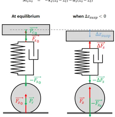
The variation of the suspension force∆Fsi applied at wheel i depends on the variation of the
length of the suspension∆zsi= zsi− zt i(see Equation (2.7a)) which itself depends only on the roll
θ and pitch φ angles (see Equation (2.7b)). The normal reaction Fziforce applied by the road on
wheel i is given by Equation (2.7c). The forces acting on the suspension are displayed in Figure2.7 where Pris the weight of the wheel (see AppendixA.3for more details).
∆Fsi = −ks∆zsi(θ,φ) − ds( ˙∆zsi(θ,φ)) (2.7a) ∆zsi(θ,φ) = ²ilwsinθ − licosθsinφ (2.7b) Fzi = Fzi0+ ∆Fsi (2.7c) where²i= ½ 1 if i = {2,4} −1 if i = {1, 3} and li= ½ lf if i = {1,2} −lr if i = {3,4} .
The nominal normal reaction force Fzi0 at equilibrium applied on wheel i is given by
Equa-tion (2.8). The demonstration is given in AppendixA.4.
Fzi0 = lrMTg 2(lf+lr) if i = {1,2} lfMTg 2(lf+lr) if i = {3,4} (2.8)
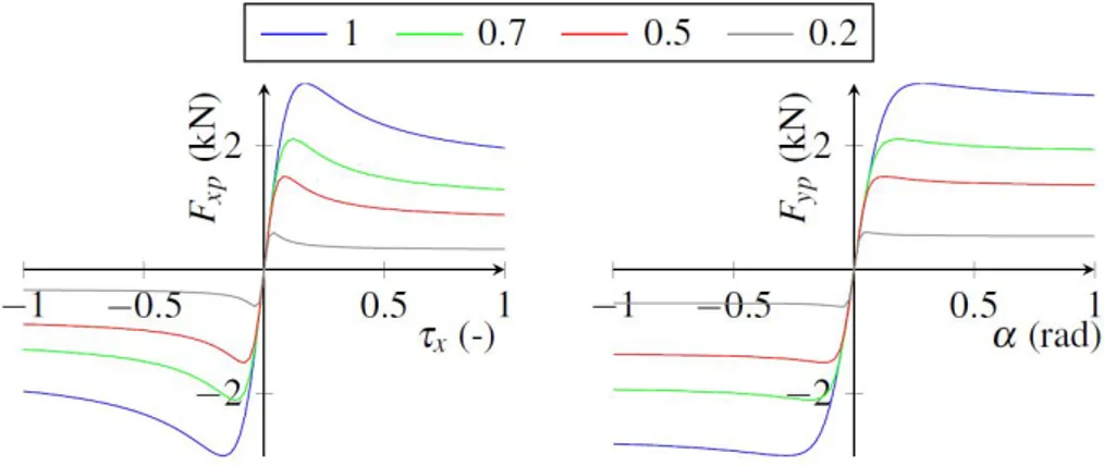
![Figure 2.9 ). The longitudinal slip ratio τ xi belongs to [−1;1], where τ xi = −1 corresponds to the sit-](https://thumb-eu.123doks.com/thumbv2/123doknet/3002196.84263/40.892.219.709.417.743/figure-longitudinal-slip-ratio-τ-belongs-corresponds-sit.webp)