CONDITIONALLY POSITIVE DEFINITE KERNELS
FOR SVM BASED IMAGE RECOGNITION
Sabri Boughorbel, Jean-Philippe Tarel, Nozha Boujemaa
Sabri.Boughorbel@inria.fr, Jean-Philippe.Tarel@lcpc.fr, Nozha.Boujemaa@inria.fr
ABSTRACTKernel based methods such as Support Vector Machine (SVM) have provided successful tools for solving many recognition problems. One of the reason of this success is the use of kernels. Positive definiteness has to be checked for kernels to be suitable for most of these methods. For in-stance for SVM, the use of a positive definite kernel insures that the optimized problem is convex and thus the obtained solution is unique. Alternative class of kernels called con-ditionally positive definite have been studied for a long time from the theoretical point of view and have drawn attention from the community only in the last decade. We propose a new kernel, named log kernel, which seems particularly interesting for images. Moreover, we prove that this new kernel is a conditionally positive definite kernel as well as the power kernel. Finally, we show from experimentations that using conditionally positive definite kernels allows us to outperform classical positive definite kernels.
1. INTRODUCTION
Support Vector Machine (SVM) [1] is one of the latest and most successful algorithm in computer vision. It is pro-viding good solutions to many image recognition problems. SVM has a solid theoretical framework [2] which helps to analyze and understand why it works so well. The basic idea behind SVM is to build a classifier that maximizes the margin between positive and negative examples. Large mar-gin classifiers have proved to yield to good generalization capacity which means a good ability to discover the true un-derlying data distribution. Formally, SVM algorithm boils down to minimize quadratic problem:
W(α) = − ` X i=1 αi+ 1 2 ` X i,j=1 αiαjyiyjK(xi, xj) (1)
with respect to Kuhn-Tucker coefficients α, under the equi-librium constraint:
`
X
i=1
αiyi= 0 (2)
Thanks to Muscle NoE for funding.
Fig. 1. Illustration of SVM recognition on a 2D toy
prob-lem in presence of outliers. Positive example are sented with white circles and negative example are repre-sented with black filled circles. Solid line represents the decision boundary of the SVM classifier. Dotted lines de-pict the edge of the margin, support vectors are surrounded and misclassified examples are crossed.
where (x1, y1), . . . , (x`, y`) ∈ X ×{±1} is the training set.
The SVM decision function f(x) ∈ {±1} is expressed as: f(x) =sign à X i∈SV α0iyiK(xi, x) + b0 ! (3) where α0
i are the optimal coefficients obtained by the
min-imization of (1). b0 is the shift coefficient which can be
computed with respect to the training set. SV is the set of indexes corresponding to non-zero α0
i since the
Kuhn-Tucker condition have to be checked: α0 i[yi( X j∈SV α0 jyjK(xj, xi) + b0) − 1] = 0.
Training examples corresponding to non-zero αiare called
support vectors.
As long as K(x, x0)is a positive definite kernel, W (α)
achieved at a unique minimum. It has been proved that for any positive definite kernel, there exists a mapping func-tion such as the kernel can be written as dot product, i.e. K(xi, xj) = Φ(xi) · Φ(xj). The function Φ usually maps
feature space X into a high dimension space.
To illustrate this, we consider the well-known example of the polynomial kernel of degree 2 on R2:
K(x, x0) = (x · x0)2 = (x1x01+ x2x02) 2 = Φ(x) · Φ(x0) with Φ : R2 → R3 , Φ(x) = (x2 1, √ 2x1x2, x22).
K(x, x0)is thus positive definite, since it can be written as
a dot product on R3. Generally, the mapping Φ is used
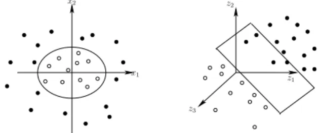
im-plicitly which means that the kernel computation does not require the explicit expression of Φ. Only definite positive-ness of the kernel must be checked. This is called the kernel trick [3]. The SVM classifier is in fact only a linear classi-fier on the mapped space, see Fig. 2. Now, let us recall the
x1 x2
z3
z1 z2
Fig. 2. 2D Data on the left is non linearly separable.
Us-ing the polynomial kernel of degree 2, data is mapped in R3on the right. The SVM separates mapped positive and
negative examples in R3 by hyperplane. This hyperplane
corresponds to a curve in R2.
definition of a positive definite kernel:
Definition 1. Let X be a nonempty set. A function K : X ×
X → R is called a positive definite kernel if and only if K is symmetric (i.e K(x, x0) = K(x0, x)for all x, x0 ∈ X )
and
n
X
j,k=1
cjckK(xj, xk) ≥ 0,
for all n ≥ 1, c1, . . . , cn∈ R, and x1, . . . xn∈ X . 2. CONDITIONALLY POSITIVE DEFINITE
KERNELS
We reviewed in the introduction how positive definite ker-nels are suitable for SVM. Looking at the equilibrium con-straint (2), it is clear that the domain to which the vector c belongs can be restrained. This remark leads to define the family of conditionally positive definite kernels [4]. In the
following, we review the main properties of this family and its connections with positive definite family.
Definition 2. Let X be a nonempty set. A kernel K is called
conditionally positive definite if and only if it is symmetric
and
n
X
j,k=1
cjckK(xj, xk) ≥ 0
for n ≥ 1, c1, . . . , cn ∈ R with Pnj=1cj = 0 and
x1, . . . , xn ∈ X .
We now give a basic example of conditionally positive definite kernel which will be of importance in the following, and we recall the proof of its definite positiveness from [4], page 69.Example:
K(x, x0) = −kx − x0k2
= −kxk2
− kx0k2
+ 2hx, x0i
Proof. To check definition 2, we consider {x1, . . . , xn} ⊆
X withPnj=1cj = 0, and we have: n X j,k=1 cjckK(xj, xk) = − n X j,k=1 cjck||xj||2 − n X j,k=1 cjck||xk||2+ 2 n X j,k=1 cjckhxj, xki = − n X k=1 ck | {z } =0 n X j=1 cj||xj||2− n X j=1 cj | {z } =0 n X k=1 ck||xk||2 + 2 n X j,k=1 cjckhxj, xki = 2 n X j,k=1 cjckhxj, xki ≥ 0
This proves that minus of the square of the Euclidean dis-tance is conditionally positive definite.
In [3], conditionally positive definite kernels are used with SVM algorithm. In the following, we explain why conditionally positive definite kernels are also suitable for SVM algorithm. We firstly recall, from [4] page 74, an im-portant relation between positive definite and conditionally positive definite kernels:
Proposition 1. Let K be a symmetric kernel on X × X .
Then for any x0∈ X , we set
˜ K(x, x0) = 1 2[K(x, x 0) − K(x, x 0) −K(x0, x0) + K(x0, x0)] (4) ˜
Kis positive definite if and only if K is conditionally
This Proposition 1 presents a strong and interesting link between positive and conditionally positive definite families since it gives a necessary and sufficient condition. It can be used with advantages when designing new kernels for SVM. From that, let us show how conditionally positive defi-nite kernels are suitable for SVM. Assume that K and ˜K are two kernels satisfying the Proposition 1. We consider the SVM problem (1) using a conditionally positive definite kernel: f W(α) = − ` X i=1 αi+ 1 2 ` X i,j=1 αiαjyiyjK(x˜ i, xj) under constraint,P`
i=1αiyi= 0. We now replace ˜Kby its
expression from (4). For any x0∈ X , we thus have:
˜
K(xi, xj) =
1
2[K(xi, xj) − K(xi, x0) −K(xj, x0) + K(x0, x0)]
Terms corresponding to K(xi, x0), K(xj, x0) and
K(x0, x0)vanish according to the constraint (2). Formally: ` X i,j=1 αiαjyiyjK(xi, x0) = ` X j=1 αjyj | {z } =0 ` X i=1 αiyiK(xi, x0) = 0. Similarly, ` X i,j=1 αiαjyiyjK(x0, xj) = 0.
Therefore, only the term corresponding to K(xi, xj)
re-mains, and we obtain: f W(α) = − ` X i=1 αi+ 1 4 ` X i,j=1 αiαjyiyjK(xi, xj) = 2W ( 1 2α) Hence fW(α)is rewritten with respect to the associated pos-itive definite kernel K only. Thus with SVM, the use a con-ditionally positive definite kernel is equivalent to the use of the associated positive definite kernel. This also proves that conditionally positive definite kernels can be used for SVM algorithm.
3. POWER AND LOG KERNELS
In this section, we investigate properties of conditionally positive definite family. We focus on two particular kernels:
· Power distance kernel introduced first in [3]:
KPower(x, x0) = −kx − x0kβ. (5)
This kernel leads to scale invariant SVM classifier, as it can be shown by direct extension of [5].
· New kernel we named Log kernel:
KLog(x, x0) = − log¡1 + kx − x0kβ¢. (6)
To prove that the above kernels are conditionally positive definite, we recall from [4] page 75 and 78:
Theorem 1. Let X be a nonempty set and let K : X ×X →
R be symmetric. Then K is conditionally positive definite if
and only if exp(uK) is positive definite for all u > 0.
Proposition 2. If K : X ×X → R is conditionally positive
definite and satisfies K(x, x) ≤ 0 for x ∈ X then so it is of
−(−K)βfor 0 < β < 1 and of − ln(1 − K).
Proof. Considering a conditionally positive definite kernel
Ksuch that K(x, y) ≤ 0 for any (x, y) ∈ X × X , then
it follows from Theorem 1 that exp(uK) is positive defi-nite, and thus conditionally positive definite. The constant kernel is obviously conditionally positive definite. Thus,
exp(uK) − 1 is conditionally positive definite as the sum of
two conditionally positive definite kernels. For 0 < β < 1 and s < 0, we can write:
−(−s)β = β Γ(1 − β) Z +∞ 0 (eus− 1) du uβ+1 − ln(1 − s) = Z +∞ 0 (eus− 1)e −u u du
Then , by replacing s with K, we can deduce that −(−K)β
and − ln(1 − K) are conditionally positive definite kernels as a sum of conditionally positive definite ones.
By applying the previous proposition to conditionally positive definite kernel K(x, x0) = −kx − x0k2introduced
in Sec. 2, we deduce that the Log (6) and Power distance (5) kernels are conditionally positive definite for 0 < β ≤ 2.
4. EXPERIMENTS
We compared performances of Power and Log kernels, for image recognition tasks. The tests have been carried on an image database containing 5 classes from Corel database, with an additional texture class of grasses, as shown in Fig. 3. Each class contains 100 images. Images are de-scribed using an RBG color histogram with a size of 43
= 64 bins. A 3-fold cross validation is applied to estimate the errors rates. We considered the recognition problem of one class-vs-the others. Comparisons are performed with
Fig. 3. Each row presents one of the 6 classes used for
experiments (castles, sun rises, grasses, mountains, birds, water falls).
respect to the following kernels: RBF kernel KRBF(x, y) =
e−kx−yk2/2σ2, Laplace kernel [6] KLap(x, y) = e−kx−yk/σ,
Power and Log kernels. Tab. 1 summarizes the average per-formances of the different kernels. We tuned two parame-ters to obtain the best validation error: 1) the SVM regu-larization coefficient and the kernel hyper-parameter (β, σ, and d) (see Fig. 4). The Log and Power kernels lead to bet-ter performances than the other kernels. Tab. 2 presents the best class confusion obtained for the Log kernel. Sunrises, Grasses and Birds classes are well recognized. Some con-fusions appear between Castles, Mountains and Waterfalls classes due to the presence of similar colors.
Kernels valid. error test error
RBF 24.38±0.54 24.33±1.06
Laplace 23.5±0.82 23.66±0.89 Power 21.88±0.15 21.44± 2.16
Log 21.77±0.20 21.12±1.70
Table 1. Average validation and test errors for the different
kernels.
castle sun grass mount bird water
castle 71 4 0 9 5 6 sun 5 84 0 0 0 0 grass 0 0 100 0 1 0 mount 12 6 0 72 3 19 bird 5 4 0 5 82 4 water 7 2 0 14 9 71
Table 2. Best class confusion matrix using the Log kernel.
0.22 0.22 0.22 0.22 0.23 0.23 0.23 0.23 0.23 0.24 0.24 0.24 0.24 0.24 0.25 0.25 0.25 0.25 0.25 0.25 0.26 0.26 0.26 0.26 0.26 0.27 0.27 0.27 0.27 0.28 0.290.3 0.31 log2(C) β −4 −2 0 2 4 6 8 10 0.2 0.4 0.6 0.8 1 1.2 1.4 1.6 1.8
Fig. 4. Average validation error with respect to log2(C)and βfor Log kernel. C is the SVM regularization coefficient.
5. CONCLUSION
We have summarized, mainly from [4], several of the im-portant properties of conditionally positive definite kernels. In particular, conditionally positive definite kernels have been proved to be suitable for SVM algorithm. Moreover, conditionally positive definite kernels have many interest-ing properties related with positive definite kernels. These properties provides very powerful tools to design both new conditionally positive definite kernels and new positive def-inite kernels. We proposed in particular a new kernel in the context of SVM, we named the Log kernel which seems to perform particularly well in our image recognition tests.
6. REFERENCES
[1] V. Vapnik, Statistical Learning Theory, Wiley, New York, 1998.
[2] B. Scholkopf and A. Smola, Learning with kernels, MIT University Press Cambridge, 2002.
[3] B. Scholkopf, “The kernel trick for distances,” in NIPS, 2000, pp. 301–307.
[4] C. Berg, J. P. R. Christensen, and P. Ressel, Harmonic Anal-ysis on Semigroups: Theory of Positive Definite and Related Functions, Springer-Verlag, 1984.
[5] F. Fleuret and H. Sahbi, “Scale invariance of support vec-tor machines based on the triangular kernel,” in Proceedings of IEEE Workshop on Stat. and Comput. Theories of Vision, Nice, France, 2003.
[6] O. Chapelle, P. Haffner, and V. Vapnik, “Svms for histogram-based image classification,” IEEE Transactions on Neural Networks, 1999. special issue on Support Vectors, 1999.